Theoretical Study of the Thermal Distribution in Yb-Doped Double-Clad Fiber Laser by Considering Different Heat Sources

Theoretical Study of the Thermal Distribution in Yb-Doped

Double-Clad Fiber Laser by Considering Different Heat Sources

Maryam Karimi*

Abstract—Thermal effects limit the gain, quality, and stability of high power fiber lasers and amplifiers. In this paper, different values of heat conductive coefficients at the core, the first and second clad with the complete form of the heat transfer equation are considered. A quartic equation was proposed to determine the temperature at the fiber laser surface. Using the surface temperature value, the temperature can be determined at the longitudinal and radial position of the double clad fiber laser. The different definitions of heat sources which were previously presented in articles is used to describe the heat generation at a double clad high pump power fiber laser condition. The results were compared to each other, and the percentage of each factor in heat generation was calculated.

1. INTRODUCTION

Doped fiber amplifiers and lasers have been considered more than that of other solid state lasers [1], because of high-quality, high-performance, gain stability, small quantum defects (QD), flexibility, low transmission loss and cavity noise, low cost, also compactness, no thermal lensing, small footprint, saturation energy, and stability to the environmental effects [2–4].

Photodarkening (PD) effect is overcome at the Ytterbium-doped glass fiber as well as undesirable effects such as pair induced quenching (PIQ) and excited state absorption that limits the dopant concentration [5, 6], which is seen more in the Erbium-doped fiber [7]. Therefore, the dopant density can be enhanced at the glass host which makes the average output power of such lasers up to kilo-watts [8– 10], so these lasers can be used to welding, cutting, surface processing military equipment [8, 11, 12], and high energy physics [13]. Thulium-doped fibers operate at a widely tunable wavelength range from 1810 to 2200 nm, which makes them suitable for many medical and military applications [14, 15]. Erbium doped fiber lasers and amplifiers are used in optical communication systems and sensors. Some effects such as clustering limit the erbium concentration in fiber medium [16]. Therefore, the output power is limited, and the thermal effects on the pulse can be ignored.

By photon absorption in the active medium and the existence of QDs, the nonradioactive decays become the heat source at high power lasers and amplifiers [14]. QD is the energy difference between the pump and signal photons converted to heat [17]. The ratio of the QD at lasers is typically less than 16% [17], and the lowest value for QD is about 0.6% for the single clad doped fiber [18]. Several phenomena appear in the active medium by heat generation, such as thermal lens [19], mechanical stresses [9], change in the refractive indices [4, 20], and consequently birefringent of the active medium [21], which causes some limitation at the output of lasers and amplifiers. In the solid-state lasers with large cross-sections, heat creates a thermal lens and causes mode instability in the fiber lasers and amplifiers [4, 22]. Study and verification of the heat distribution in the fiber lasers is the first step to prediction and control of the several effects in high power fiber lasers and amplifiers. At the

Received 15 August 2018, Accepted 23 October 2018, Scheduled 5 November 2018 * Corresponding author: Maryam Karimi ([email protected]).

lasers with large cross-sections such as rod type Nd-YAG laser, usually cooling is done by water, but at the fiber lasers and amplifiers cooling is done using the surrounding air.

Heat transfer in the medium is with three processes: conduction, convection and radiation, described with Fourier’s, Newton’s, and Stefan-Boltzman’s laws respectively. In this paper assuming that the heat inside the fiber propagates only by the conduction transfer and in the fiber surface, the heat transfer is done by radiation and conduction. The fiber medium is homogeneous and elastic.

There are many theoretical studies on Ytterbium-doped fiber laser (YbDFL) based on rate equations [13]. In the high power fiber lasers by assuming a large value for the dopant concentration with respect to the upper state level, the rate equations have a analytical or quasi-analytical solution [2, 23– 25]. Shooting method with different algorithms can give the most exact solution for the boundary value problems [26, 27], but the stability of the solution depends on the initial values [28]. The simple superfluorescent model (SSM) for describing the gain in active fibers is the simplest method that gives a fast and exact solution with Newton-Raphson or Runge-Kouta algorithms [28]. This model is based on two assumptions. In the first, the fluorescence or laser spectrum assumed is a real (not complex) function of frequency. This assumption for the Lorentzian line, shape process is valid. So in the SSM the absorption coefficient is omitted from the relations. The second assumption is that at high pump power and saturated regime, the output spectrum will be narrow and line wide; therefore, the integral over the frequency at the gain equation can be omitted, and only the central frequency is entered in calculations [29]. In most articles, the existence of other transition modes in the laser or amplifier is ignored [28], and in practice, making loops on cavity can prevent the propagation of upper modes in the active medium.

2. ATOMIC RATE EQUATIONS IN DOUBLE CLAD FIBER LASER

By considering a three-level laser system with a fast decay of third level and a steady-state regime that the populations are time-invariant, the variations of the ground and upper levels are given as [30]:

N1 =N

1 +W21

1/τ +R+W12+W21

,

N2 =N

R+W12

1/τ +Rτ +W12+W21

,

(1)

where W12 and W21 are the stimulated absorption and emission rates of signal power between levels 1

and 2, and R is the absorption rate of pump power and expressed as follows [29]:

W21(r, z) =

σeP(z)ψ(r)

hυπω2 ,

W12(r, z) =

σaτ P(z)ψ(r)

hυπω2

,

R(r, z) = σ

a

pPp(z)ψp(r)

hυpπωp2

,

(2)

Since in the double clad fiber lasers and amplifiers (DCFL-A), the pump power is injected at the core

and the first clad region, ω = ₀2π_rr₌₀=Rcoψ(r, θ)drdθ/π, ωp =₀2π_rr₌₀=Rcl1ψp(r, θ)drdθ/π, where

Rco and Rcl1 are the core and the first clad radius, respectively, and ψ and ψp are the qualitative

patterns of the pump and laser with the Gaussian envelopes. So the state transition probability at the Eq. (2), for the bidirectional pump scheme, will be as follows:

W21(r, z) =

ΓpσeP+(z) +P+(z)

hυAcl1

,

W12(r, z) =

ΓσaP+(z) +P+(z)

hυAcl1

,

R(r, z) = Γpσ

a

pPp+(z) +Pp+(z)

hυpAco ,

The overlap factor at each wavelength is the fraction of the power that is actually coupled to the active region and is defined as Γi =_θθ₌₀=2π_rr₌₀=Rcoθ(r, θ) ¯ψi(r, θ)drdθ, where θ(r), ¯ψi(r, θ) are the dopant and

power distributions at each wavelength respectively, and Rco is the dopant distribution radius which is often equal to the core radius [31, 32]. ¯ψi(r, θ) = ψi(r, θ)/_θθ₌₀=2π_rr₌₀=Riψi(r, θ)drdθ, here Ri indicates

the power distribution in each wavelength. For the signal (laser) wavelength Ri = Rco and for the pump power Ri =Rcl1. For the signal power with the Gaussian pulse envelope, the profile variation

is proportional to |Ex|2 and can approximate as ψi(r, ωi) = exp(−r2/ω2_i)/πω_i2 by integration, and the overlap factor will be [29, 33, 34]:

Γi= Pcore

Ptotal

= 1−exp−2R2_i/ω2_i (4)

wherePcore,Ptotal, andRi are the spot size (ωi) for any modes and defined as [14, 27]:

ωi =RJ0(Ui)

Vi

Ui

K1(Wi)

K0(Wi)

(5)

where V = √U2_+W2 _{= koan}2

1−n22, W = a

β2−_k2

on22 = V

√

b, U = ak2

on21−β2 = V

√ 1−b, and b=W2_/V2 _{[9, 34]. n}

1 and n2 are the refractive indices of the core and the first clad, respectively;

β is the mode propagation constant; k0 = 2π/λ0 is the wave number in the free space; λ0 is the free

space wavelength. The refractive index in any wavelength is obtained from the Sellemier equation for GeO2/SiO2 glass in the whole wavelength region by [35]:

n2_s = 1 +

3

i=1

[SAi+x(GAi−SAi)]λ20

λ2₀−[SLi+x(GLi−SLi)]2 (6)

x is the molar fraction of GeO2, and SAi,SLi,GAi, andGLi are coefficients of the Sellemier equation

for SiO2 and GeO2 glasses, respectively [35]. Table 1 represents the coefficients numerical values of the

Sellemier equation.

Table 1. Sellimeier coefficients for Silica and Germania glass [36].

SiO2

SA1 SL1 SA2 SL2 SA3 SL3

0.6961663 0.0684043 0.4079426 0.1162414 0.8974794 9.896161

GeO2

GA1 GL1 GA2 GL2 GA3 GL3

0.80686642 0.068972606 0.71815848 0.15396605 0.85416831 11.841931

In analytical definition of the effective mode diameter (ωi) the mode propagation constant,β, must

be calculated from the fiber eigenvalue equation at any propagation mode, then the values of theV,U,

W are replaced at Eq. (5). If only the LP01 mode or V number in the range of 0.8–2.8 is considered,

for the Gaussian pulse shape, the experimental relation approximate of the spot size in the doped fiber can be used as follows [34, 35]:

ωi =ρ

0.616 + 1.66

V1.5 +

0.987

V6 (7)

In [37] various forms of Eq. (7) are presented for different pulse shapes. The overlap factor for pump power in a double clad fiber laser is estimated as Γp ≈Aco/Acl1 [38, 39]. In Eqs. (1)–(3), σe, σa, and

σ_pa are emission and absorption cross-section of lasing, and absorption cross-section of pump power, respectively; τ is the steady-state lifetime; ψp, ψ are considered as top hat profile; N is the dopant

concentration in ion/m3. In the general case, the variations of signal (laser) and pump power are described as follows [40].

±dP±(z, υi)

dz = Γ[(σ

e

+σa)N2(z, υi, υj)−σaN]P±(z, υi)+2hυi

Δυ n Γσ

e

N2(z, υi, υj)−αP±(z, υi) (8)

±dPp±(z, υj)

dz = Γp

σe_p+σ_paN2(z, υi, υj)−σapN

where αp and α are background loss at the pump and laser wavelength, respectively. For the narrow band wide pulse, the frequency dependence of pump and signal power can be ignored in Eqs. (8)– (9) [29]. At the high pump power and saturation regime, the frequency distributions of N2(z, υi, υj)

may be assumed to be narrower than unsaturated line width. So in this case, only the central frequency is considered [29, 41]. Then the rate equations are reduced to [42]:

±dP±(z)

dz = Γ[(σ

e

+σa)N2(z)−σaN]P±(z)−αP±(z) (10)

±dPp±(z)

dz = −Γp

σa_pN−σe_p+σ_paN2(z)

P_p±(z)−αpP_p±(z) (11)

N2(z)

N =

P_p+(z) +P_p−(z)σ_paΓp

hυpAco +

P+(z) +P−(z)σaΓ

hυAco

P_p+(z) +P_p−(z) σ_pa+σe_pΓp

hυpAco +

1

τ +

P+(z) +P−(z)(σa +σe) Γ

hυAco

(12)

The gain of fiber laser is defined as [26, 43]:

Gain = exp

0

(g(z)−αL)dz (13)

in which the gain coefficient at the lasing wavelength is given by [2, 43]:

g(z)≡Γ[(σe+σa)N2(z)−σaN] (14)

In the high pump power regime N2 N, so Eq. (11) is converted to [2, 40]:

±dPp±(z)

dz =−Γpσ

a

pN Pp±(z)−αpP_p±(z) (15)

So, the analytical solution of Eq. (15) for the forward and backward pump powers will be as follows [2]:

P_p+(z)∼=P_p+(0) exp−ΓpσpaN −αpz (16)

P_p−(z)∼=P_p−(L) exp−ΓpσapN −αp(L−z) (17)

Generally, αa = ΓpσpaN is called the core absorption coefficient at the pump wavelength [29, 44]. At

the strong power fiber laser the pump absorption cross-section can be ignoredσe_p∼= 0, andσa σe, so

Pp(z)σapΓp/τ + (Γ(σe +σa)/hυAco)(P+(z) +P−(z)), and therefore g(z) in Eq. (14) can be [23]:

g(z)∼= g0(z)

1 +P+(z) +P−(z)/Psat (18)

where Psat = hυAco/Γσeτ and g0(z) =

NΓpσa(P_p+(z)+P_p−(z))υ

Psatυp −NΓσ

a

, so the rate in Eqs. (10)–(11)

for the double clad high power laser with bidirectional pump scheme becomes:

dP+(z)

dz = N

Γp·σ_pa·υ·P_p+(0) exp(−αz) +P_p−(L) exp (−α(L−z))/(P sat·υp)−Γσa

1 +P+(z) +P−(z)/Psat P

+

(z)

−αP+(z) (19)

dP−(z)

dz = −N

Γp·σ_pa·υ·P_p+(0) exp (−αz) +P_p−(L) exp (−α(L−z))/(P sat·υp)−Γσa

1 +P+(z) +P−(z)/Psat P

+

(z)

+αP+(z) (20)

For a side-pump fiber laser, one of the termsP_p+(z) orP_p−(z) must be omitted from the rate equations. In Eqs. (19)–(20), α = αa+αp. Our work is similar to the simplified analytical solutions with the

and the real values of core and clad cross-sections appear in the equations. Superfluorescent model is based on the two assumptions. Firstly, the imaginary part of fluorescence is negligible. In other words, the environment has no absorption in lasing wavelength. Secondly, in the saturation regime the output spectrum is much narrow and linear in which the other frequencies can be eliminated from the equations. In this work, we ignore other transverse traveling modes in the fiber. Coiling of doped fiber can be used to eliminate the higher order modes [45, 46].

3. STATIC THERMAL MODEL IN DOUBLE CLAD FIBER LASERS

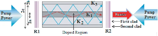
To have a laser or amplifier with high output and brightness, a double clad scheme is used [3]. Figure 1 shows a double clad fiber laser with bidirectional end pump schematically. The use of double clad doped fibers to increase pump efficiency is proposed in 1988 [3, 47].

Figure 1. Schematic illustration of double clad fiber laser with bidirectional pump.

To improve pump absorption and increase the fraction of cladding modes overlap with the active core area, the rotational symmetry of the first clad must be broken with different shapes of first clad cross-section, in which high power, low brightness pump light is launched into a large cross-section and numerical aperture of the clad [3]. In the present paper, a simple circular shape is considered, and the generated light is efficiently trapped inside the core. The effect of the coating or the fiber jacket is ignored. By considering the steady-state condition in fiber laser and propagation of the fundamental mode in the cavity, the effect of mode instability can be ignored. The threshold of the mode instability depends on different parameters such as fiber laser length, dopant concentration, seed power, frequency, and co-dopants in fiber lasers [48–50, 67]. For the Yb doped fiber laser with cavity length about 20 m and pump power lower than 500 W, this assumption can be accurate.

4. DIFFERENT DEFINITION OF HEAT SOURCE IN FIBER LASERS AND AMPLIFIERS

The thermal distribution in the DCFL can be described by the thermal conduction equation in the cylindrical coordinate [33, 51].

1

r ∂ ∂r

r∂T(r, z) ∂r =−

Q(r, z)

K , (21)

heat source the quantum defect is introduced as the main source of heat production [56]. The quantum defect heat arises from the energy difference between the pump and signal photons or spontaneously emitted photon [4]. On the other hand, the difference between pump and signal (lasing) energy causes

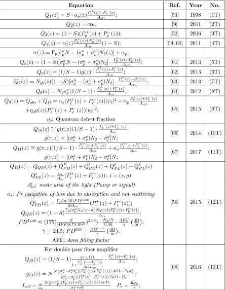
Table 2. Different formulas for the heat distribution.

Equation Ref. Year No.

Q1(z) =S·αp(z)P +

p(z)+P_p−(z)

A_cl1 ; [53] 1998 (1T)

Q2(z) =cte; [9] 2001 (2T)

Q3(z) = (1−S)(Pp+(z) +Pp−(z)); [52] 2006 (3T)

Q4(z) =α(z)P +

p(z)+Pp−(z)

Aco (1−S); [54, 60] 2011 (4T)

α(z) = Γp[σa_pN −(σ_pe+σ_pa)N2(z)] +αp;

Q5(z) = (1−S)[σpaN −(σpa+σpe)N2]·P +

p(z)+Pp−(z)

A_cl1 ; [61] 2013 (5T)

Q6(z) = (1/S−1)g(z)·

P+

(z)+P−(z)

Aco ; [62] 2013 (6T)

Q7(z) =Nyb(z)(1−S)[σpa−(σpa+σpe)N2]·

P+

p(z)+P_p−(z)

A_cl1 ; [63] 2013 (7T)

Q8(z) =N2σe(1/S−1)·P +

(z)+P−(z)

Aco ; [64] 2012 (8T)

Q9(z) =Qabs+QD =αs(P+(z) +P−(z))|ψ|2+αpP +

p(z)+P_p−(z)

A_cl1

+ηqg(z)(P+(z) +P−(z))|ψ|2; [65] 2015 (9T)

ηq: Quantum defect fraction

Q10(z)∼=g(r, z)(1/S−1)·

P+(z)+P−(z)

Aco ; _{[66] 2014 (10T)}

g(r, z) = [(σa +σe)N2−σa]N;

Q11(z)∼=g(r, z)(1/S−1)·

P+(z)+P−(z)

Aco +αs

P+(z)+P−(z)

Aco ; _{[67] 2017 (11T)}

g(r, z) = [(σa +σe)N2−σa]N;

Q12(z) =QQD(z) +QP_{P D}(z) +Q_{P D}(z) +Qp_{P L}(z) +Q_{P L}(z)

[56] 2015 (12T)

Qi_{P L}(z) = _Aαii m(P

+

i (z) +Pi−(z)); i= (s, p)

Ai_m: mode area of the light (Pump or signal)

αi: Pr opagation of loss due to absorption and not scattering

Qi_{P D}(z) = ΓiLn(10)_10AP D1µm

co (P +

i (z) +Pi−(z));

QQD(z) = (1−S)Γp(σ

a

pN1(z)−σ_peN2(z))(Pp+(z)+Pp−(z))

Aco ;

P D1µm≈(175(_{AF F·8}N_.74·1025)2.09)· N₀2_.46/N ·AF F_γ dB_m;

γ = 24.5;P D633 = P D_γ1µm dB_m; AFF:Area filling factor

For double pass fiber amplifier

[68] 2016 (13T)

Q13(z) = (1/S−1) gJ·L(z) 1+P

+

(z)+P−(z) AcoIsat

· P+(z)+P−(z)

Aco ;

g13(z) =N

(σa_pσe_s−σa_sσe_p)(P_p+(z)+P_p−(z))/Acl1−Pτσsa (σ_pa+σe_p)(P_p+(z)+P_p−(z))/Acl1+Pτ ;

Isat= _ωω_p(σ

a

p+σe_p)(Pp+(z)+Pp−(z))/Acl1+Pτ

σa

s+σes Pτ = ωp

heating the medium by spontaneous emission in the infrared region. The photon wavelength of the laser is longer than the pump photon wavelength, so this shift is called as Stokes shift [57]. The second source of heat is photodarkening loss which can increase the temperature [4, 56, 58], which depends on the pump and signal wavelengths, seed power, fiber core size, etc. [56]. The photodarkening loss is about 6–7% of the all loss, but it decreases the transverse mode instability threshold [50, 56]. The last heat source corresponds to background loss or gray loss of path [56, 59], that is the propagation loss (PL) in pump and signal (lasing) wavelengths. The different formulations of heat density are listed in Table 2. The difference between the equations in Table 2 depends on considering the different factors for heat generation and how these factors are defined. In Eq. (12T) all of the factors that are contributed to heat generation, namely QD, PD, and PL are considered, so it is a complete form of heat generation equations at the fiber lasers and amplifiers. In all of the equations, the QD factor is presented, although different mathematical definitions of the QD are considered. In Eqs. (9T), (11T) the relationship depends on the laser (signal) power, but in Eqs. (4T), (5T) the pump power is used in the mathematical definition. In Eqs. (4T), (9T), and (11T), the effect of background loss in heat generation is considered which is separately the PL-P in Eq. (4T), the PL-S in Eq. (9T), and both of PL-P and PL-S in Eq. (11T).

All of the formulas in Table 2 are adjusted by this assumption that the dopant distribution of the core is uniform and has the top hat profile of the pump power. The dependence of the heat distribution on the radial coordinate can be ignored, so the Q function is not relevant to the radial parameters ‘r’ and ‘φ’. In Table 2, S is the quantum efficiency or optical conversion efficiency which is λp/λ in

theory [13, 51, 54]. α(z) is the absorption coefficient of pump power and can be calculated by [13, 51, 59]:

α(z) = Γpσa_pN−σe_p+σ_paN2(z)

+αp (22)

The effect of the pump power or dopant distribution can be calculated numerically by the multilayer method or the analytical integration of the heat distribution in the core [69, 70].

5. SOLVING HEAT TRANSFER EQUATION WITH CONSIDERING OF

RADIATIVE AND CONVECTIVE HEAT TRANSFER IN DOUBLE CLAD FIBER LASERS OR AMPLIFIERS

The heat transfer equation in the core region is expressed as follows:

1

r ∂ ∂r

r∂Tcore(r, z) ∂r =−

Q(z)

K1

, (0≤r ≤a) (23)

For the cladding regions a≤r≤c, there is no heat source andQ(z) = 0; so, for the cladding region: 1

r ∂ ∂r

r∂Tclads(r, z)

∂r = 0, (a≤r≤c) (24)

where Tcore and Tclads are the temperatures at the core and cladding regions, respectively. The

temperature and its derivatives must be continuous across the inner boundaries. Moreover, at the outer cladding-air interface, heat is transferred by convective and radiative heat flux [54, 71]. So at boundaries, the following conditions are confirmed:

dTcore(r = 0, z)/dr= 0 → Tcore(r = 0, z) =cte, (25)

Tcore(a, z) =Tclad1(a, z), K1

dTcore(r=a, z)

dr =K2

dTclad1(r=a, z)

dr , (26)

Tclad1(b, z) =Tclad2(b, z), K2

dTclad1(r =b, z)

dr =K3

dTclad2(r =b, z)

dr , (27)

dTclad2(r=c, z)

dr =

h

Kh(Tc(r, z)−Tclad2(r=c, z)) +

σbε Kh

T_c4(r, z)−T_clad24 (r=c, z), (28)

wherehis the heat transfer coefficient. The value ofhdepends on the environment temperature [52]. In this paper by assuming a constant value for the environment temperature, a constant value is considered for the heat transfer coefficient. The values of K1,K2,K3 are the conductive heat transfer coefficients

of the air. Tcore, Tclad1, and Tclad2 are the temperature variation at the core, first and second clads,

respectively, and Tc is the environment temperature or the temperature that fiber laser sustained. σb

is the Stefan-Boltzmann constant, and ε is the surface emissivity. Each of Eqs. (26) and (27) consists of two boundary conditions (the temperature and its derivative are continuous at the boundaries). So there are six boundary conditions that determine all the constant values. By solving Eqs. (23) and (24) using boundary conditions, the value ofTclad2 at the radial pointr =c is obtained as follows:

f(Tclad2(r =c, z)) =

σbε

KhT

4

clad2(r =c, z) +

h

KhTclad2(r=c, z)−

σbε

KhT

4

c −

h KhTc+

Q(z)a2

2K3c

= 0 (29)

The quartic functions have an analytical solution such as Ferrari’s solution, Cardano’s casus irreducibilis of three real roots, and alternative cubic resolvent due to Descartes, Euler, and Lagrange [72]. In this paper, the numerical Newton-Raphson Method is used to solve it.

Using Tclad2 and boundary condition in Eq. (25), the temperature value at the fiber center is

determined as follows:

T0(z) =Tclad2(r =c, z) +

Q(z)a2

4K1

+Q(z)a

2

K2

ln (b/a) +Q(z)a

2

K3

ln (c/b), (30)

So the temperature changes in the core and clads as follows:

Tcore(r, z) =T0(z)−

Q(z)r2

4K1

(0≤r≤a), (31)

Tclad1(r, z) =−

Q(z)a2

K2

lnr+Q(z)a2lnb

1

k2−

1

k3

+Tclad2(r=c, z)+

Q(z)a2

K3

lnc (a≤r ≤b),(32)

Tclad2(r, z) =−

Q(z)a2

K3

lnr+Q(z)a

2

K3

lnc+Tclad2(r=c, z) (b≤r≤c), (33)

6. SIMULATION RESULTS AND DISCUSSIONS

In this paper, only a bidirectional pump configuration with top hat profile is considered for continuous wave condition. The pump and laser wavelengths areλp = 925 nm andλ= 1090 nm, respectively. The

laser length, L = 20 m, and the grating reflection coefficients at the ends of the fiber,R1 and R2, are

0.99 and 0.04, respectively. In the present paper it is assumed that there is no Bragg reflector at the pump wavelength. In other wordsR3 = 0 [32, 73]. The other parameter values, such as cross-sections,

first and second clad radii, steady-state lifetime, background losses, and input pump power, are given in Table 3.

The refractive index of the glass at signal wavelength 1090 with 6%, mole GeO2 (x = 7%), using

Eq. (6) is 1.4583. For the fiber with 10µm core radius, V number of the signal is 2.3248. On the other hand, at this wavelength the laser operates as the single mode. The overlap factor is determined from Eq. (7), about 0.813 at the lasing wavelength. The fast and stable algorithm is used to obtain numerical answers [28]. The complete form of rate in Eqs. (10)–(11) is solved using Runge-Kouta method and considering boundary conditionsP+=R1P−, and P− =R2P+ in the iterative algorithm.

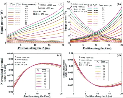
In Figure 2, the results of forward and backward of the signal and pump power, also normalized densities of Metastable and ground-state level vs. the position along the fiber length are depicted.

As shown in Figure 2(a), by increasing pump power (bidirectional pumping), the forward and backward signal powers are increased. At any pump power, the values ofP+(0) andP−(0) are coincident with each other in the first point of the fiber. If the reflection coefficient at the input end of laser “R1”

is about 0.8, then at the z = 0, the value of P−(0) is placed slightly lower than that of P+(0). In Figure 2(b), the variations ofP_p+(0) andP_p−(0) with respect to Z are shown. At any pump power, the variations ofP_p+andP_p− have a symmetric form with respect to a line passing through the fiber center. The reason for the symmetry of the forward and backward pumps is the assumption of the absence of reflector (mirror or grating) at the end of the fiber at the pump wavelength. By considering a value for the reflectivity of the output coupler at the pump wavelength (R3), this symmetry will disappear [44].

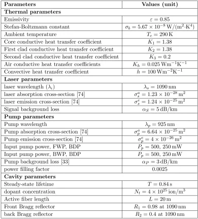
Table 3. Parameter values used in the of thermal effects simulation at Yb DDCFL.

Parameters Values (unit)

Thermal parameters

Emissivity ε= 0.85

Stefan-Boltzmann constant σb = 5.67×10−8W/(m2·K4)

Ambient temperature Tc = 290 K

Core conductive heat transfer coefficient K1 = 1.38

First clad conductive heat transfer coefficient K2 = 1.38

Second clad conductive heat transfer coefficient K3 = 0.2

Air conductive heat transfer coefficients Kh= 0.025 Wm−1K−1

Convective heat transfer coefficient h= 100 Wm−2K−1 Laser parameters

laser wavelength (λι) λs= 1090 nm

laser absorption cross-section [74] σa_s = 1.23×10−28m2 laser emission cross-section [74] σ_se= 1.24×10−25m2 Signal background loss αS = 5 dB/km

Pump parameters

Pump wavelength λp= 925 nm

Pump absorption cross-section [74] σa_p = 6.64×10−25m2 Pump emission cross-section [74] σe_p = 4×10−26m2 Input pump power, FWP, BDP Pp = 500, 250 mW

Input pump power, BWP, BDP Pp = 500, 250 mW

Pump background loss [33] αP = 3 dB/km

power filling factor 0.0025

Cavity parameters

Steady-state lifetime T = 0.84 s dopant concentration Nt= 4×1025ion/m3

Active fiber length L= 20 m

Front Bragg reflector R1= 0.98 at 1090 nm

back Bragg reflector R2= 0.4 at 1090 nm

respect to fiber position are illustrated in Figures 2(c) and 2(d), respectively. If there are no reflectors at the ends of the fiber, similar to the fiber amplifiers, the maximum value of the normalized density of each level must be unity [32]. So the reflectivity of the mirrors at the signal and pump wavelengths determine the shape of the graph. As shown in Figure 2, by increasing the pump power, the ground state density decreases, and the upper state density naturally increases. When the reflector with high reflective index coefficient “R1” is placed at the input end of the fiber, the photons at the signal (lasing)

wavelength are not allowed to exit from the fiber input end. Photon imprisonment at the input end of fiber causes decreasing the emission probability of photons in signal (lasing) wavelength at this point of the fiber. In other words, it is expected that the density of the upper level is higher at the input end of the fiber; Figure 2(d) confirms the expectation. At the midpoint of the fiber, the pump powers have lower values, so one expects that the density of the second level must be a minimum value as shown in Figure 2(d). The values of the first level density in Figure 2(c) are obtained fromN−N2, and the laser

output power is obtained from Pout =P+(1−R2) [23].

(a) (b)

(c) (d)

Figure 2. Variation of (a) lasing power, (b) pump power, (c) normalized ground state densities, (d) normalized upper state density versus position along the fiber.

(a) (b)

Figure 3. Laser output power as a function of input power, (a) different reflectivity at the input end of the laser, (b) different dopant density.

the input refractive index coefficient, the value of the output power increases. For larger values of input power, the effect of refractive indexR1has greater impact on the output of the fiber laser. By increasing

the dopant concentration in the doped fiber, the output power increases at any input power value. Since the active fiber length is L = 20 m, by increasing the concentration higher than 6×1025 _{the output}

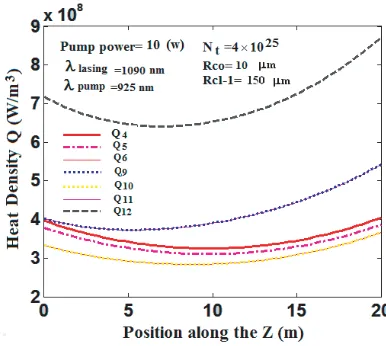
Figure 4. Heat variation along the fiber position in the bidirectional pump scheme with different descriptions of heat generated in Table 2.

Figure 5. Different factor share in the heat generation at the fiber laser with the relative large first clad size.

The variations of heat density along the axial direction of the fiber for the different heat generation definitions of Table 2 are shown in Figure 4. Using any Table 2’s equations to determine the heat generation density by the parameter values of the Table 3, the results have the values between 108–109. As seen in Figure 4, the values of Q6 and Q10 from Eqs. (6T) and (10T) are overlapping and have

minimum values with respect to other curves. As shown in Table 2, they are equal to each other, and only the values of the gain factor and signal powers have a role on that. It is notable that these curves are not symmetric with respect to perpendicular line passed through the fiber center. ButQ4 and Q5

curves are symmetric with respect to this line. The reason is the definition of their functions in Table 2, which depend on the pump powers. As seen in Figure 2(b), P_p+ and P_p− have symmetry with respect to the line passing through the fiber center, but P+ and P− have no symmetry. So if pump power (intensity) has a role in the definition of the heat generation equation, it is expected that the heat simulation results must have symmetry with respect to this line in the bidirectional pump scheme; the results of Q4 and Q5 in Figure 4 agree with this expectation. In Eq. (4T), the background loss at the

pump wavelength is considered in heat generation, so it is expected that the value ofQ4 is larger than

clad area, which must be incorrect in the study of the double clad fiber laser. The curves ofQ9 andQ11

do not coincide with each other, but their results are close with each other. In the calculation of Eq. (9), we consider ηq = 1 in the simulation. As seen in Eqs. (9T) and (10T), the heat generation depends

on signal (lasing) intensity. Since the curves of P− and P+ are not symmetric with respect to the line passing through the fiber center, it is expected that the values of Q9 and Q11 have no symmetry. The

last curve Q12 has the largest value among the curves of Figure 4. As shown in Eq. (12T), all of the

factors that participate in heat generation are considered which make Eq. (12T) the complete form of the equation to heat generation. It must be noticed that Γp/Aco is equal to 1/Acl1, so the contribution

of the pump power in the first clad is considered in Eq. (12). In this paper Eq. (13) is not drawn, because the relation is defined for the amplifier.

In the circular graph of Figure 5, the percentage of each factor contribution (sources) in the heat production at the fiber laser with the special condition indicated in Table 3 is shown. As shown in the graph, for the double clad fiber laser with relatively large first clad (rcl1 > 10rco), the effects of

background loss and PD on the pump wavelength share less than 1%. Most of the generated heat is related to QD, and the portion of the PD effect on the signal (lasing) wavelength for the heat generation is about 32%. The background loss at the signal wavelength has about 17% share in heat generation. It should be noted that this graph is obtained by averaging the total fiber length. The contribution of each factor depends on the location in the fiber laser; also by changing the size of the first clad (making smaller), it is expected that the contribution of the PD and background loss at pump wavelength will be increased.

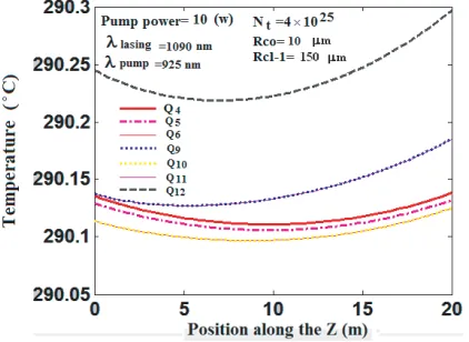
To determine the temperature at any point in the fiber, after solving the rate equations and calculating pump and signal (lasing) powers at any longitudinal distance of the fiber, the quartic Eq. (29) must be solved. In this paper, the Newton-Raphson method is used to solve this equation. Since f(Tclad2(r =c), z) is a quartic function with a high slope, using the Secant or Newton-Raphson

method increases the speed of the calculation in comparisons to other numerical methods. By solving Eq. (29), the temperature values at r =c are evaluated for different definitions of the heat generation in Table 2. The results are shown in Figure 6. The trends of temperature variations are similar to the heat generation in Figure 4. Using any of the heat generation relationships presented in Table 2, the temperature difference between different points of the fiber surface is about one percent of centigrade.

Figure 6. Temperature variation of the fiber laser surface (r=c), with respect to the fiber position in the bidirectional pump scheme and different descriptions of heat generated.

Eq. (12T) was considered the all known factors that contribute to heat generation. So it is the most complete form of equations to describe heat generation in the fiber lasers and amplifiers. That is expected for simulation of heat distribution in the low power fiber lasers without consideringQi_{P D}, and

Qi_{P L} gives similar results by using Eq. (12T). In the following of this paper, only the complete form of heat generation Eq. (12T) is used for simulation. By evaluatingT0, from Eq. (30), the temperature can

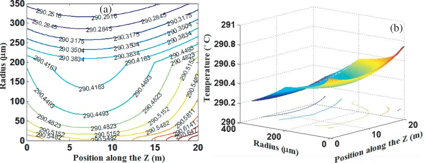
(a)

(b)

Figure 7. (a) Isothermal regions, (b) 3D variations of the temperature with respect to the fiber length and the fiber radius.

(a) (b)

Figure 8. Temperature variations with respect to: (a) the core radius, (b) the position along the fiber.

are shown for different positions of fiber lengths and fiber radii. Figure 7(b) shows 3D variations of the temperature with respect to fiber length and radial direction. As shown in Figure 7(b), the temperature decreases along the radial direction of the fiber. By cooling the fiber surface, a temperature gradient occurs between the core region and the fiber surface, which causes the heat to flow out of the fiber laser. Figure 8(a) shows the variation of temperature with respect to core radius at different laser length. As shown in Figures 4 and 8(b), the heat or temperature distribution is not symmetric relative to the longitudinal axes of the fiber. As already mentioned the reason is the existence of the reflectors at the ends of fiber with the different reflection coefficients. The temperature has the maximum value at

L= 20 m (the end of fiber), which points out that at high power fiber laser the possibility of thermal damage at the end of fiber laser (output end) is much higher due to the enhancement of the temperature at the endpoint. The temperature may damage the fiber laser when the temperature is approaching 150∼200◦C [75]. The smallest value of the graph occurs aroundL= 8 m. The reason of curves break off in the boundary regions between the first and second clads is thermal conductivity coefficient difference in these regions. The variations of the temperature with respect to the longitudinal position for different core radii are shown in Figure 8(b), in which the black curve shows the maximum temperature values at the central axis of the fiber.

(b) (a)

Figure 9. Variation of the central axis temperature with respect to: (a) the position along the fiber for the different input power, (b) the input pump power for the different fiber radius.

power about 18 W, the temperature at the fiber input increases approximately about 1.2◦C, while in the same condition, the output temperature increases about 1.4◦C. At the same pump power difference, the temperature at the middle region increases about 1◦C.

The variations of the central axis temperature with respect to the dopant concentration are depicted in Figure 10. Increasing the dopant concentration in the core causes the increase of the fiber temperature, which acts similarly to the increase of pump power. It should be noted that the temperature linearly changes with the pump power, but the temperature acts as second-degree function of the dopant concentration.

(a) (b)

Figure 10. Temperature variation at the central axis of fiber with respect to: (a) the position along the fiber for the different dopant concentration, (b) the dopant concentration for the different fiber radius.

7. CONCLUSION

In this paper, the complete form of the heat transfer function by considering the conductive and radiative heat transfer is used for determining the heat distribution in the fiber laser.

Different definitions of the heat source at fiber lasers, which had been depicted in the previous papers, are rewritten at the table, and the simulation results of them for the heat generation at the fiber laser with the bidirectional pump scheme were compared to each other.

By considering only the bidirectional pump scheme at fiber laser and the pump and lasing wavelength at 925 and 1090 nm respectively, the variations of the pump and lasing power and also population density at the stable and upper level with respect to the position of the fiber laser for different pump powers were compared with each other. The effect of the input reflection coefficient and the dopant density of the fiber laser output were determined.

In the fiber laser with respectively large first clad (rcl1>10rco), the percentages of various factors

in the heat production were determined. In general, the effect of the quantum defect in the heat generation is the maximum. But in the large first clad fiber laser, the effects of the background loss at the pump wavelength and the pump photodarkening are less than 1% at the heat generation. The signal photodarkening and background loss at the signal wavelength have shared about 32% and 17%, respectively.

The variations of temperature with respect to radial and longitudinal position in the fiber laser were determined and compared with each other. The temperature was linearly changed with the input power, but the temperature variations with respect to the dopant density had a quadratic function. The effects of pump power and dopant concentration on the distribution of the fiber laser were studied.

REFERENCES

1. Liao, K. H., A. G. Mordovanakis, B. Hou, G. Chang, M. Rever, G. Mourou, J. Nees, and A. Galvanauskas, “Generation of hard X-rays using an ultrafast fiber laser system,” Opt. Express, Vol. 15, 13942–13948, 2007.

2. Kelson, I. and A. Hardy, “Optimization of strongly pumped fiber lasers,” J. Ligthwave Technol., Vol. 17, 891–897, 1999.

3. Zervas, M. N. and C. A. Codemard, “High power fiber lasers: A review,” IEEE J. Select. Topic. Quant. Electron., Vol. 20, 0904123, 2014.

4. ˇSuˇsnjar, P., V. Agreˇz, and R. Petkovˇsek, “Photodarkening as a heat source in ytterbium doped fiber amplifiers,”Opt. Express, Vol. 26, 6420-642615265-15277, 2018.

5. Engholm, M., L. Norin, C. Hirt, S. T. Fredrich-Thorntonc, K. Petermannc, and G. Huberc, “Quenching processes in Yb lasers correlation to the valence stability of the Yb ion,” Proc. of SPIE, Vol. 7193, 71931U-1, 2009.

6. Ward, B., “Theory and modeling of photodarkening induced quasi static degradation in fiber amplifiers,”Opt. Express, Vol. 24, 3488–3501, 2016.

7. Ding, M. and P. K. Cheo, “Dependence of ion-pair induced self-pulsing in Er-doped fiber lasers on emission to absorption ratio,”IEEE. Photon. Technol. Lett., Vol. 8, 1627–1629, 1996.

8. Huang, L., H. Zhang, X. Wang, and P. Zhou, “Diode-pumped 1178-nm high-power Yb-doped fiber laser operating at 125 C,”IEEE Photonics Journal, Vol. 8, 1501407, 2016.

9. Brown, D. C. and H. J. Hoffman, “Thermal, stress, and thermo-optic effects in high average power double-clad silica fiber lasers,” IEEE J. Quant. Electron., Vol. 37, 207–217, 2001.

10. Oron, R. and A. A. Hardy, “Rayleigh backscattering and amplified spontaneous emission in high-power Ytterbium-doped fiber amplifiers,”J. Opt. Soc. Am. B, Vol. 16, 695–801, 1999.

11. Kaushal, H. and G. Kaddoum, “Applications of lasers for tactical military operations,” Digital Object Identifier 10.1109/ACCESS, Vol. 5, 20736–20753, 2017.

12. Dong, L. and B. Samson,Fiber Lasers: Basics, Technology, and Applications, CRC Press, printed on acid-free paper, 2017.

13. Shao, H., K. Duan, Y. Zhu, H. Yan, H. Yang, and W. Zhao, “Numerical analysis of Ytterbium-doped double-clad fiber lasers based on the temperature-dependent rate equation,”Optik, Vol. 124, 4336–4340, 2013.

15. Baravets, Y., F. Todorov, and P. Honzatko, “High-power thulium-doped fiber laser in an all-fiber configuration,” Proceedings of the SPIE, Vol. 10142, id. 101420G 4, 2016.

16. Wagener, J. L., P. F. Wysocki, M. J. F. Digonnet, H. J. Shaw, and D. J. Digiovanni, “Effects of concentration and clusters in erbium-doped fiber lasers,” Opt. Lett., Vol. 18, 2014–2016, 1993. 17. Dawson, J. W., M. J. Messerly, R. J. Beach, M. Y. Shverdin, E. A. Stappaerts, A. K. Sridharan,

P. H. Pax, J. E. Heebner, C. W. Siders, and C. P. J. Barty, “Analysis of the scalability of diffraction-limited fiber lasers and amplifiers to high average power,”Opt. Express, Vol. 16, 13240–13266, 2008. 18. Yao, T., J. Ji, and J. Nilsson, “Ultra-low quantum-defect heating in Ytterbium-doped

aluminosilicate fibers,”J. Lightwav. Technol., Vol. 32, 429–434, 2014.

19. Rimington, N. W., S. L. Schieffer, W. Andreas Schroeder, and B. K. Brickeen, “Thermal lens shaping in Brewster gain media: A high-power, diode-pumped Nd:GdVO4 laser,” Opt. Express, Vol. 12, 1426–1436, 2004.

20. Kuznetsov, M. S., O. L. Antipov, A. A. Fotiadi, and P. M´egret, “Electronic and thermal refractive index changes in Ytterbium-doped fiber amplifiers,”Opt. Express, Vol. 21, 22374–22388, 2013. 21. Sabaeian, M. and H. Nadgaran, “Investigation of thermal dispersion and thermally-induced

birefringence on high-power double clad Yb:glass fiber laser,”International Journal of Optics and Photonics (IJOP), Vol. 2, 25–31, 2008.

22. Kong, F., J. Xue, R. H. Stolen, and L. Dong, “Direct experimental observation of stimulated thermal Rayleigh scattering with polarization modes in a fiber amplifier,” LET Optica, Vol. 3, 975–978, 2016.

23. Kelson, I. and A. A. Hardy, “Strongly pumped fiber lasers,” IEEE J. Quant. Electron., Vol. 34, 1570–1577, 1998.

24. Xiao, L., P. Yan, M. Gong, W. Wei, and P. Ou, “An approximate analytic solution of strongly pumped Yb-doped double-clad fiber lasers without neglecting the scattering loss,”Opt. Commun., Vol. 230, 401–410, 2004.

25. Hardy, A., “Signal amplification in strongly pumped fiber amplifiers,”IEEE. J. Quant. Electron., Vol. 33, 307–313, 1997.

26. Karimi, M. and A. H. Farahbod, “Improved shooting algorithm using answer ranges definition to design doped optical fiber laser,”Opt. Commun., Vol. 324, 212–220, 2014.

27. Hu, X., T. Ning, L. Pei, and W. Jian, “Novel shooting method with simple control strategy for fiber lasers,”Optik, Vol. 125, 1975–1979, 2014.

28. Luo, Z., C. Ye, G. Sun, Z. Cai, M. Si, and Q. Li, “Simplified analytic solutions and a novel fast algorithm for Yb3+-doped double-clad fiber lasers,” Opt. Commun., Vol. 277, 118–124, 2007. 29. Digonnet, M. J. F., “Theory of superfluorescent fiber lasers,”J. Lightwave Technol., Vol. 4, 1631–

1639, 1986.

30. Desurvire, E., Erbium Doped Fiber Amplifiers: Principles and Applications, Wiley, New York, 1994.

31. Karimi, M., N. Granpayeh, and M. K. Moravvej Farshi, “Analysis and design of the dye doped polymer optical fiber amplifiers,”Appl. Physics B, Vol. 78, 387–396, 2004.

32. Brunet, F., Y. Taillon, P. Galarneau, and S. Larochelle, “Practical design of double-clad Ytterbium-doped fiber amplifiers using Giles parameters,”IEEE J. Quant. Electron., Vol. 40, 1294–1300, 2004. 33. Yan, P., X. Wang, Y. Huang, C. Fu, J. Sun, Q. Xiao, D. Li, and M. Gong, “Fiber core mode leakage induced by refractive index variation in high-power fiber laser,” Chin. Phys. B, Vol. 26, 034205, 2017.

34. Agrawal, G. P., Fiber-optic Communication Systems, 3rd Edition, A John Wiley & Sons, Inc., 2002.

35. Karimi, M., “Optimization of core size in erbium doped holey fiber amplifiers,” Optik, Vol. 125, 2780–2783, 2014.

37. Marcuse, D., “Loss analysis of single-mode fiber splices,” The Bell System Technology Journal, Vol. 56, 703–718, 1977.

38. Leproux, P. and S. F´evrier, “Modeling and optimization of double-clad fiber amplifiers using chaotic propagation of the pump,”Optical Fiber Technol., Vol. 6, 324–339, 2001.

39. Kouznetsov, D. and J. V. Moloney, “Highly efficient, high-gain, short-length, and power-scalable incoherent diode slab-pumped fiber amplifier/laser,”IEEE J. Quant. Electron., Vol. 39, 1452–1461, 2003.

40. Quintela, M. A., C. Lavin, M. Lomer, A. Quintela, and J. M. Lopez-Higuera, “Superfluorescent erbium doped fiber optic sources comparative study,” Proc. of SPIE, Vol. 5952, 1–10, 2005. 41. Casperson, L. W. and A. Yariv, “Spectral narrowing in high-gain lasers,” IEEE J. Quantum.

Electron., Vol. 8, 80, 1972.

42. Xiao, L., P. Yan, M. Gong, W. Wei, and P. Ou, “An approximate analytic solution of strongly pumped Yb-doped double-clad fiber lasers without neglecting the scattering loss,”Opt. Commun., Vol. 230, 401–410, 2004.

43. Pask, H. M., R. J. Carman, D. C. Hanna, A. C. Tropper, C. J. Mackechnie, P. R. Barber, and J. M. Dawes, “Ytterbium-doped silica fiber lasers: Versatile sources for the 1–1.2 pm region,”IEEE J. Selected Top. in Quant. Electron., Vol. 1, 2–13, 1995.

44. Lim, C. and Y. Izawa, “Modeling of end-pumped CW quasi-three-level lasers,” IEEE J. Quant. Electron., Vol. 38, 306–311, 2002.

45. Kong, F., C. Dunn, J. Parsons, M. T. Kalichevsky-Dong, T. W. Hawkins, M. Jones, and L. Dong, “Large-mode-area fibers operating near singlemode regime,” Opt. Express, Vol. 24, 10295–10301, 2016.

46. Wielandy, S., “Implications of higher-order mode content in large mode area fibers with good beam quality,”Opt. Express, Vol. 15, 15402–15409, 2016.

47. Snitzer, E., H. Po, F. Hakimi, R. Tumminelli, and B. C. McCollum, “Double-clad, offset core Nd fiber laser,” The Opt. Fiber Commun. Conf., New Orleans, LA, PD5, 1988.

48. Jauregui, C., H. J. Otto, S. Breitkopf, J. Limpert, and A. T¨unnermann, “Optimizing the mode instability threshold of high-power fiber laser systems,” Proc. of SPIE, Fiber Lasers XIII: Technology, Systems, and Applications, Vol. 9728, 97280B, 2015.

49. Otto, H. J., N. Modsching, C. Jauregui, J. Limpert, and A. T¨unnermann, “Impact of photodarkening on the mode instability threshold,”Opt. Express, Vol. 23, 15265–15277, 2015. 50. Jauregui, C., H. J. Ottoa, C. Stihler, J. Limpert, and A. T¨unnermann, “The impact of core

co-dopants on the mode instability threshold of high-power fiber laser systems,” Proc. of SPIE, Fiber Lasers XIV: Technology and Systems, Vol. 10083, 100830N, 2017.

51. Li, J., K. Duan, Y. Wang, X. Cao, W. Zhao, Y. Guo, and X. Lin, “Theoretical analysis of the heat dissipation mechanism in Yb3+-doped double-clad fiber lasers,” J. Modern Optic, Vol. 55, 459–471, 2008.

52. Yan, P., A. Xu, and M. Gong, “Numerical analysis of temperature distributions in Yb-doped double-clad fiber lasers with consideration of radiative heat transfer,”Opt. Engin., Vol. 45, 124201, 2006.

53. Davis, M. K., M. J. F. Digonnet, and R. H. Pantell, “Thermal effects in doped fibers,”J. Lightwave Technol., Vol. 16, 1013–1022, 1998.

54. Li, J., Y. Chen, M. Chen, H. Chen, X. Jin, Y. Yang, Z. Dai, and Y. Liu, “Theoretical analysis and heat dissipation of mid-infrared chalcogenide fiber Raman laser,” Opt. Commun., Vol. 284, 1278–1283, 2011.

55. Lapointe, M. A., S. Chatigny, M. Pich´e, M. C. Skaff, and J. N. Maran, “Thermal effects in high-power CW fiber lasers,” Proc. SPIE Fiber Lasers VI: Technology, Systems, and Applications, Vol. 7195, 1U, 2009.

57. Lood, F. and N. P. Kherani, “Influence of luminescent material properties on stimulated emission luminescent solar concentrators (SELSCs) using a 4-level system,” Opt. Express, Vol. 25, A1023, 2017.

58. Ward, B., “Theory and modeling of photodarkening induced quasi static degradation in fiber amplifiers,”Opt. Express, Vol. 24, 3488–3501, 2016.

59. Kuznetsov, M. S., O. L. Antipov, A. A. Fotiadi, and P. M´egret, “Electronic and thermal refractive index changes in Ytterbium-doped fiber amplifiers,”Opt. Express, Vol. 21, 22374–22388, 2013. 60. Abouricha, M., A. Boulezhar, and N. Habiballah, “The comparative study of the temperature

distribution of fiber laser with different pump schemes,”O. J. Metal, Vol. 3, 64–71, 2013.

61. Naderi, S., I. Dajani, T. Madden, and C. Robin, “Investigations of modal instabilities in fiber amplifiers through detailed numerical simulations,”Opt. Express, Vol. 21, 16111–16129, 2013. 62. Hansen, K. R., T. T. Alkeskjold, J. Broeng, and J. Lægsgaard, “Theoretical analysis of mode

instability in high-power fiber amplifiers,” Opt. Express, Vol. 21, 1944–1971, 2013.

63. Smith, A. V. and J. J. Smith, “Increasing mode instability thresholds of fiber amplifiers by gain saturation,” Opt. Express, Vol. 21, 15168–15182, 2013.

64. Ward, B., C. Robin, and I. Dajani, “Origin of thermal modal instabilities in large mode area fiber amplifiers,”Opt. Express, Vol. 2, 11407–11422, 2012.

65. Ward, B. G., “Accurate modeling of rod-type photonic crystal fiber amplifiers,” Proc. of SPIE, Vol. 9728, 97280F-1, 2015.

66. Tao, R., P. Ma, X. Wang, P. Zhou, and Z. Liu, “1.3 kW monolithic linearly polarized single-mode master oscillator power amplifier and strategies for mitigating mode instabilities,” Photon. Res., Vol. 3, 86–93, 2015.

67. Tao, R., X. Wang, P. Zhou, and Z. Liu, “Seed power dependence of mode instabilities in high power fiber amplifiers,”J. Opt., 103667.R1, 2017.

68. Lægsgaard, J., “Static thermo-optic instability indouble-pass fiber amplifiers,” Opt. Express, Vol. 24, 13429–13443, 2016.

69. Gong, M., Y. Yuan, C. Li, P. Yan, H. Zhang, and S. Liao, “Numerical modeling of transverse mode competition in strongly pumped multimode fiber lasers and amplifiers,” Opt. Express, Vol. 15, 3236–3246, 2007.

70. Mohammed, Z., H. Saghafifar, and M. Soltanolkotabi, “An approximate analytical model for temperature and power distribution in high power Yb-doped double clad fiber lasers,”Laser Phys., Vol. 24, 115107, 2014.

71. Sabaeian, M., H. Nadgaran, M. De Sario, L. Mescia, and F. Prudenzano, “Thermal effects on double clad octagonal Yb:glass fiber laser,”Optical Materials, Vol. 31, 1300–1305, 2009.

72. Neumark, S., Solution of Cubic and Quartic Equations, 1st Edition, Pergam on Press, Oxford, London, 1965.

73. Kelson, I. and A. Hardy, “Optimization of strongly pumped fiber lasers,”J. of Ligthwave Technol., Vol. 17, 891–897, 1999.

74. Pask, H. M., R. J. Carman, D. C. Hanna, A. C. Tropper, C. J. Mackechnie, P. R. Barber, and J. M. Dawes, “Ytterbium-doped silica fiber lasers: Versatile sources for the 1–1.2 pm region,”IEEE. J. of Quant. Electron., Vol. 1, 2–13, 1995.