The Cryptographic Power of Random Selection
Matthias Krause and Matthias Hamann
Theoretical Computer Science University of Mannheim
Mannheim, Germany
Abstract. The principle of random selection and the principle of adding biased noise are new paradigms used in several recent papers for con-structing lightweight RFID authentication protocols. The cryptographic power of adding biased noise can be characterized by the hardness of the intensively studied Learning Parity with Noise (LPN) Problem. In analogy to this, we identify a corresponding learning problem for ran-dom selection and study its complexity. Given L secret linear func-tionsf1, . . . , fL:{0,1}n−→ {0,1}a,RandomSelect(L, n, a) denotes the
problem of learning f1, . . . , fL from values (u, fl(u)), where the secret
indicesl∈ {1, . . . , L}and the inputsu∈ {0,1}n
are randomly chosen by an oracle. We take an algebraic attack approach to design a nontrivial learning algorithm for this problem, where the running time is domi-nated by the time needed to solve full-rank systems of linear equations overO nL
unknowns. In addition to the mathematical findings relating correctness and average running time of the suggested algorithm, we also provide an experimental assessment of our results.
Keywords: Lightweight Cryptography, Algebraic Attacks, Algorithmic Learning, Foundations and Complexity Theory
1
Introduction
The very limited computational resources available in technical devices like RFID (radio frequency identification) tags implied an intensive search for lightweight authentication protocols in recent years. Standard block encryption functions like Triple-DES or AES seem to be not suited for such protocols largely because the amount of hardware to implement and the energy consumption to perform these operations is too high (see, e.g., [7] or [17] for more information on this topic).
The principle of adding biased noise to the output of a linear basis function underlies the HB-protocol, originally proposed by Hopper and Blum [16] and later improved to HB+ by Juels and Weis [17], as well as its variants HB# and
Trusted-HB (see [13] and [6], respectively). The protocols of the HB-family are provably secure against passive attacks with respect to the Learning Parity with Noise Conjecture but the problem to design HB-like protocols which are secure against active adversaries seems to be still unsolved (see, e.g., [14], [20], [12]).
The principle of random selection underlies, e.g., the CKK-protocols of Ci-cho´n, Klonowski, and Kuty lowski [7] as well as the Ff-protocols in [3] and the Linear Protocols in [18]. It can be described as follows.
Suppose that the verifier Alice and the prover Bob run a challenge-response authentication protocol which uses a lightweight symmetric encryption operation
E:{0,1}n×K −→ {0,1}m
of block lengthn, whereKdenotes an appropriate key space. Suppose further thatEis weak in the sense that a passive adversary can efficiently compute the secret key K∈ K from samples of the form (u, EK(u)). This is obviously the case ifE is linear.
Random selection denotes a method for compensating the weakness ofE by using the following mode of operation. Instead of holding a singleK∈ K, Alice and Bob share a collection K1, . . . , KL of keys from K as their common secret information, where L > 1 is a small constant. Upon receiving a challenge u∈ {0,1}n from Alice, Bob chooses a random indexl∈ {1, . . . , L} and outputs the response y=E(u, Kl). The verification ofy with respect toucan be efficiently done by computingE−K1
l(y) for all l= 1, . . . , L.
The main problem this paper is devoted to is to determine the level of security which can be reached by applying this principle of random selection.
Note that the protocols introduced in [7], [3], and [18] are based on random selection ofGF(2)-linear functions. The choice of linear basis functions is moti-vated by the fact that they can be implemented efficiently in hardware and have desirable pseudo-random properties with respect to a wide range of important statistical tests.
It is quite obvious that, with respect to passive adversaries, the security of protocols which use random selection of linear functions can be bounded from above by the complexity of the following learning problem referred to as
RandomSelect(L, n, a): Learn GF(2)-linear functions f1, . . . , fL : {0,1}n −→ {0,1}a from values (u, fl(u)), where the secret indices l ∈ {1, . . . , L} and the inputs u ∈ {0,1}n are randomly chosen by an oracle. In order to illustrate this notion, we sketch in appendix B how an efficient learning algorithm for
RandomSelect(L, n, a) can be used for attacking the linear (n, k, L)+-protocol
described by Krause and Stegemann [18].
In recent years, people from cryptography as well as from complexity and coding theory devoted much interest to the solution of learning problems around linear structures. Prominent examples in the context of lightweight cryptography are the works by Goldreich and Levin [15], Regev [21], and Arora and Ge [2]. But all these results are rather connected to the Learning Parity with Noise Problem. To the best of our knowledge, there are currently no nontrivial results with respect to the particular problem of learning randomly selected linear functions, which is studied in the present paper.
We are strongly convinced that the complexity of RandomSelect also de-fines a lower bound on the security achievable by protocols using random se-lection of linear functions, e.g., the improved (n, k, L)++-protocol in [18]. Thus,
the running time of our algorithm hints at how the parameters n, k, and L
should be chosen in order to achieve an acceptable level of cryptographic secu-rity. Note that choosing n = 128 and L = 8 or n = 256 and L = 4, solving
RandomSelect(L, n, a) by means of our algorithm implies solving a system of around 228unknowns, which should be classified as sufficiently difficult in many practical situations.
The paper is organized as follows. In sections 2, 3, and 4, our learning algo-rithm, which conducts an algebraic attack in the spirit of [22], will be described in full detail. We represent the L linear basis functions as assignments A to a collection X = xlii=1,...,n,l=1,...,L of variables taking values from the field
K =GF(2a). We will then see that each example (u, f
l(u)) induces a
degree-L equation of a certain type in the X-variables, which allows for reducing the learning problemRandomSelect(L, n, a) to the problem of solving a system of degree-Lequations overK. While, in general, the latter problem is known to be NP-hard, we can show an efficient way to solve this special kind of systems.
One specific problem of our approach is that, due to inherent symmetries of the degree-Lequations, we can never reach a system which has full linear rank with respect to the corresponding monomials. In fact, this is the main difference between our learning algorithm and the well-known algebraic attack approaches for cryptanalyzing LFSR-based keystream generators (see, e.g., [19], [8], [9], [1]). We circumvent this problem by identifying an appropriate setT(n, L) of basis polynomials of degree at mostLwhich allow to express the degree-Lequations as linear equations overT(n, L). The choice ofT(n, L) will be justified by Theorem 2 saying that if|K| ≥L, then the system of linear equations overT(n, L) induced by all possible examples has full rank|T(n, L)|. (Note that according to Theorem 1, this is not true if|K|< L.) Our experiments, which are presented in section 5, indicate that if |K| ≥L, then with probability close to one, the number of examples needed to get a full rank system overT(n, L) exceeds|T(n, L)|only by a small constant factor. This implies that the effort to compute the uniqueweak
solutiont(A) = (t∗(A))t∗∈T(n,L) corresponding to thestrongsolutionA equals
the time needed to solve a system of|T(n, L)|linear equations over K.
But in contrast to the algebraic attacks in [19], [8], [9], [1], we still have to solve another nontrivial problem, namely, to compute the strong solution
so-lution. An efficient way to do this will complete our learning algorithm for
RandomSelect(L, n, a) in section 4. Finally, we also provide an experimental evaluation of our estimates using the computer algebra system Magma [5] in section 5 and conclude this paper with a discussion of the obtained results as well as an outlook on potentially fruitful future work in section 6.
2
The Approach
We fix positive integers n, a, L and secret GF(2)-linear functions f1, . . . , fL : {0,1}n−→ {0,1}a. The learner seeks to deduce specifications off1, . . . , fL from an oracle which outputs in each round an example (u, w)∈ {0,1}n× {0,1}a in the following way. The oracle chooses independently and uniformly a random inputu∈U {0,1}
n
, then chooses secretly a random indexl∈U [L]¬, computes
w=fl(u) and outputs (u, w).
It is easy to see that RandomSelect can be efficiently solved in the case
L= 1 by collecting examples u1, w 1
, . . . ,(um, w
m) until
u1, . . . , um contains a basis of GF(2)n. The expected number of iterations until the above goal is reached can be approximated byn+ 1.61 (see, e.g., the appendix in [11]).
We will now treat the caseL >1, which immediately yields a sharp rise in difficulty. First we need to introduce the notion of apure basis.
Definition 1. Let us call a set V = u1, w1
, . . . ,(un, wn) of n examples a pure basis, if
u1, . . . , un is a basis ofGF(2)n and there exists an indexl∈[L]
such that wi =fl ui
is satisfied for alli= 1, . . . , n.
Recalling our preliminary findings, we can easily infer that form∈Ln+Ω(1), a set of m random examples contains such a pure basis with high probability. Moreover, note that for a given set ˜V = u˜1,w˜1
, . . . ,(˜un,w˜n) the pure basis property can be tested efficiently. The respective strategy makes use of the fact that in case of a random example (u, w), where u=L
i∈Iu˜
i and I⊆[n], the
probability pthat w=L
i∈Iw˜i holds is approximatelyL
−1 if ˜V is pure and at
most (2·L)−1otherwise. The latter estimate is based on the trivial observation that if ˜V is not a pure basis, it contains at least one tuple ˜uj,w˜
j,j ∈[n], which would have to be exchanged to make the set pure. As j ∈I holds true for half of all possible (but valid) examples, the probability thatw=L
i∈Iw˜iis fulfilled although ˜V is not pure can be bounded from above by (2·L)−1.
However, it seems to be nontrivial to extract a pure basis from a set of
m∈Ln+Ω(1) examples. Exhaustive search among all subsets of sizenyields
¬For a positive integerN, we denote by [N] the set{1, . . . , N}. LetB =
v1, . . . , vn denote a basis spanning the vector spaceV. It is a simple
algebraic fact that every vectorv∈V has a unique representationI⊆[n] overB, i.e.,
v=L
i∈Iv i
a running time exponential inn. This can be shown easily by applying Stirling’s formula® to the corresponding binomial coefficient m
n
.
We exhibit the following alternative idea for solvingRandomSelect(L, n, a) for L > 1. Let e1, . . . , en denote the standard basis of the GF(2)-vector space {0,1}n and keep in mind that{0,1}n =GF(2)n ⊆Kn, where K denotes the fieldGF(2a). For all i= 1, . . . , nandl= 1, . . . , L let us denote byxl
ia variable overK representingfl ei
. Analogously, let Adenote the (n×L)-matrix with coefficients inKcompletely defined byAi,l=fl ei
. Henceforth, we will refer to
Aas astrong solution of our learning problem, thereby indicating the fact that its coefficients fully characterize the underlying secret GF(2)-linear functions
f1, . . . , fL.
Observing an example (u, w), where u= L i∈Ie
i, the only thing we know
is that there is some index l ∈[L] such that w=L
i∈IAi,l. This is equivalent to the statement that Ais a solution of the following degree-L equation in the
xli-variables.
M
i∈I
x1i ⊕w
!
·. . .· M i∈I
xLi ⊕w
!
= 0. (1)
Note that equation (1) can be rewritten as
M
J⊆I,1≤|J|≤L0
L M
j=|J|
wL−jtJ,j=wL, (2)
L0 = min{L,|I|}, where the basis polynomialstJ,j are defined as
tJ,j=
M
g,|dom(g)|=j,im(g)=J
mg
for allJ ⊆[n], 1≤ |J| ≤L, and allj,|J| ≤j≤L. The corresponding monomials
mg are in turn defined as
mg= Y
l∈dom(g)
xlg(l)
for all partial mappingsg from [L] to [n], wheredom(g) denotes the domain of
g andim(g) denotes its image.
LetT(n, L) ={tJ,j|J ⊆[n],1≤ |J| ≤L,|J| ≤j ≤L}denote the set of all basis polynomials tJ,j which may appear as part of equation (2). Moreover, we define
Φ(a, b) = b X
i=0
a
i
®Stirling’s formula is an approximation for large factorials and commonly written
n!≈√2πn n e
for integers 0≤b≤aand write
|T(n, L)|= L X
j=1
n
j
(L−j+ 1)
= (L+ 1) (Φ(n, L)−1)− L X
j=1
n
n−1
j−1
= (L+ 1) (Φ(n, L)−1)−nΦ(n−1, L−1). (3)
Consequently, each set of examples V =
u1, w
1, . . . ,(um, wm) yields a
system of m degree-L equations in the xl
i-variables, which can be written as
m K-linear equations in the tJ,j-variables. In particular, the strong solution
A∈Kn×L satisfies the relation
M(V)◦t(A) =W(V), (4)
where
– Kn×L denotes the set of all (n×L)-matrices with coefficients fromK,
– M(V) is an (m× |T(n, L)|)-matrix built by themlinear equations of type (2) corresponding to the examples inV,
– W(V)∈Km is defined byW(V) i=w
L
i¯ for alli= 1, . . . , m,
– t(A)∈KT(n,L)is defined byt(A) = (tJ,j(A))J⊆[n],1≤|J|≤L,|J|≤j≤L.
Note that in section 3, we will treat the special structure ofM(V) in further detail. Independently, it is a basic fact from linear algebra that ifM(V) has full column rank, then the linear system (4) has the unique solutiont(A), which we will call the weak solution.
Our learning algorithm proceeds as follows:
(1) Grow a set of examplesV untilM(V) has full column rank|T(n, L)|. (2) Compute the unique solutiont(A) of system (4), i.e., the weak solution of our
learning problem, by using an appropriate algorithm which solves systems of linear equations overK.
(3) Compute the strong solutionA fromt(A).
We discuss the correctness and running time of steps (1) and (2) in section 3 and an approach for step (3) in section 4.
¯Keep in mind that, unlike for the previously introducedK-variables x1
s, . . . , xLs, s∈[n], the superscriptedL in case ofwLi is not an index but an exponent. See, e.g.,
3
On Computing a Weak Solution
Let n and L be arbitrarily fixed such that 2 ≤ L ≤ n holds. Moreover, let V ⊆ {0,1}n×Kdenote a given set of examples obtained through linear functions
f1, . . . , fL : {0,1} n
−→ K, where K = GF(2a). By definition, for each tuple (u, w) ∈ V, where u=L
i∈Ie
i and I ⊆[n] denotes the unique representation of u over the standard basis e1, . . . , en of {0,1}n
, the relation w = fl0(u) =
L
i∈Ifl0 eiis bound to hold for some l0 ∈[L]. We denote by Kmin ⊆ K the
subfield ofKgenerated by all valuesfl ei
, wherel∈[L] andi∈[n]. Note that
w∈Kmin for all examples (u, w) induced byf1, . . . , fl.
In the following, we show that our learning algorithm is precluded from suc-ceeding if the secret linear functions f1, . . . , fL happen to be of a certain type or ifK itself lacks in size.
Theorem 1 If Kmin
< L, then the columns of M(V) are linearly dependent
for any set V of examples, i.e., a unique weak solution does not exist.
Proof: Let n, K, L, and f1, . . . , fL be arbitrarily fixed such that 2 ≤
Kmin
< L≤nholds and letV denote a corresponding set of examples. Obvi-ously, for each tuple (u, w)∈ V, whereu=L
i∈Ie
i andI ⊆[n], the two cases 1∈I and 1∈/I can be differentiated.
If 1∈ I holds, then it follows straightforwardly from equation (2) that the coefficient with coordinates (u, w) and t{1},(L−1) in M(V) equals wL−(L−1) =
w1. Analogously, the coefficient with coordinates (u, w) and t
{1},(L−|Kmin|) in
M(V) equalswL−(L−|Kmin|) =w|Kmin|. Note thatt{1},(L−|Kmin|)is a valid (and
different) basis polynomial as
|{1}|= 1≤ L− Kmin
≤(L−2)<(L−1)< L
holds for 2≤ |Kmin|< L. AsKmin ⊆K is a finite field of characteristic 2, we
can apply Lagrange’s theorem and straightforwardly conclude that the relation
z1 = z|Kmin| holds for all z ∈ Kmin (including 0 ∈ Kmin). Hence, if 1 ∈ I
holds for an example (u, w), then in the corresponding row of M(V) the two coefficients indexed byt{1},(L−1)and t{1},(L−|Kmin|) are always equal.
If 1∈/ I holds for an example (u, w), then the coefficient with coordinates (u, w) and t{1},(L−1) in M(V) as well as the coefficient with coordinates (u, w)
andt{1},(L−|Kmin|)in M(V) equals 0. Consequently, if Kmin
< L holds, then the column of M(V) indexed by
t{1},(L−1)equals the column indexed by t{1},(L−|K|) for any set V of examples,
i.e.,M(V) can never achieve full column rank.
Corollary 1 IfK is chosen such that|K|< L, then the columns of M(V)are linearly dependent for any set V of examples, i.e., a unique weak solution does not exist.
This will be achieved by introducing the ((2n|K|)× |T(n, L)|)-matrix M∗ =
M({0,1}n×K), which clearly corresponds to the set of all possible examples, and showing that M∗ has full column rank|T(n, L)|ifL≤ |K|holds.
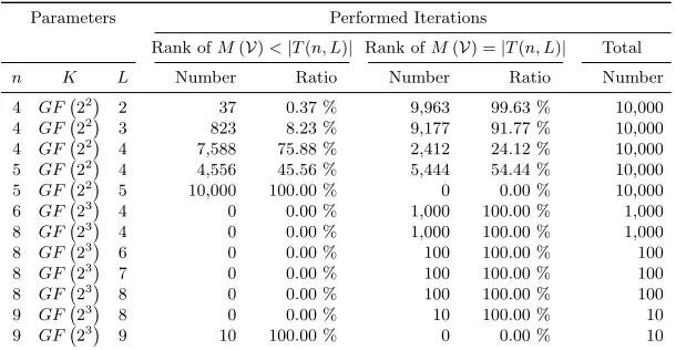
However, be careful not to misinterpret this finding, which is presented below in the form of Theorem 2. The fact thatM∗ has full column rank |T(n, L)|by no means implies that, eventually, this will also hold forM(V) if only the corre-sponding set of observationsV is large enough. In particular, the experimental results summarized in section 5 (see, e.g., table 1) show that there are cases in which the rank of M(V) is always smaller than |T(n, L)|, even if L ≤ |K| is satisfied andV equals the set{(u, fl(u)) |u∈ {0,1}
n
, l∈[L]} ⊆ {0,1}n×K°
of all possiblevalid examples.
Still, as a counterpart of Theorem 1, the following theorem proves the pos-sibility of existence of a unique weak solution for arbitrary parameters n and
L satisfying 2≤L ≤n. In other words, choosingT(n, L) to be the set of ba-sis polynomials does not necessarily lead to systems of linear equations which cannot be solved uniquely.
Theorem 2 Let n andL be arbitrarily fixed such that 2 ≤L≤n holds. If K
satisfiesL≤ |K|, then M∗ has full column rank|T(n, L)|.
Proof:We denote by Z(n) the set of monomials zd0 0 ·. . .·z
dn
n , where 0 ≤
di ≤ |K| −1 for i = 0, . . . , n. Obviously, the total number of such monomials is |Z(n)| = |K|n+1. Let us recall the aforementioned fact that the relation
z1=z|K|holds for all z∈K (including 0∈K). This straightforwardly implies that each monomial in the variables z0, . . . , zn is (as a function from Kn+1 to
K) equivalent to a monomial in Z(n). Let µJ,j denote the monomial µJ,j =
z0L−jQ
r∈Jzr for all J ⊆ [n] and j, 0 ≤ j ≤ L. The following lemma can be easily verified:
Lemma 2.1 For allJ ⊆[n],1 ≤ |J| ≤ L, and j, |J| ≤ j ≤L, and examples
(u, w)∈ {0,1}n×K, it holds thatµJ,j(w, u)equals the coefficient inM∗ which
has the coordinates(u, w)andtJ,j.
For i = 1, . . . ,|K|, we denote by ki the i-th element of the finite field K. Moreover, we suppose the convention that 00= 1 inK. Let (u, w) be an example
defined as above and keep in mind that we are treating the case L ≤ |K|. It should be observed that the coefficients in the corresponding equation of type (2) are given by wL−j, where 1 ≤j ≤ L. Thus, the set of possible exponents {L−j|1≤j≤L} is bounded from above by (L−1) < L ≤ |K|. It follows straightforwardly from Lemma 2.1 that the (distinct) columns ofM∗are columns of the matrix W⊗B⊗n, where
W =kji
i=1,...,|K|,j=0,...,|K|−1 and B=
1 0 1 1
.
°It can be seen easily that for random linear functions f
1, . . . , fL, the relation
{(u, fl(u)) |u∈ {0,1}n, l∈[L]} 6= {0,1}n×K will always hold if L < |K| and is
As W andB are regular, W ⊗B⊗n is regular, too. This, in turn, implies that the columns ofM∗ are linearly independent, thus proving Theorem 2.
We will see in section 4 that for |K| ∈ O dnL4, the strong solution can be reconstructed from the weak solution in timenO(L)with error probability at mostd−1. Furthermore, section 5 will feature an experimental assessment of the number of random (valid) observations needed untilM(V) achieves full column rank|T(n, L)| for various combinations ofn,L, andK (see table 2).
4
On Computing a Strong Solution from the Unique
Weak Solution
Letn,K,L, andf1, . . . , fLbe defined as before. Remember that the goal of our learning algorithm is to compute a strong solution fully characterized by the L
sets
ei, f l ei
|i∈[n] ,l= 1, . . . , L, whereeidenotes thei-th element of the standard basis ofGF(2)n andfl ei
=xli∈K. Obviously, this information can equivalently be expressed as a matrixA∈Kn×L defined byA
i,·= x1i, . . . , xLi
for alli= 1, . . . , n.
Hence, we have to solve the following problem: Compute the matrix A ∈
Kn×L from the informationt(A), where
t(A) = (tJ,j(A))J⊆[n],1≤|J|≤L,|J|≤j≤L
is the unique weak solution determined previously. But before we lay out how (and under which conditions) a strong solution A can be found, we need to introduce the following two definitions along with an important theorem linking them:
Definition 2. Let for all vectors x∈KL the signature sgt(x) of x be defined assgt(x) = (|x|k)k∈K, where |x|k denotes the number of components ofxwhich equal k.
Furthermore, consider the following new family of polynomials:
Definition 3. a) For allL≥1 andj≥0 let the simple symmetric polynomial
sj over the variablesx1, . . . , xL be defined by s0= 1 and
sj= M
S⊆[L],|S|=j
mS,
wheremS =Qi∈Sxi for allS⊆[L]. Moreover, we denote
s(x) = (s0(x), s1(x), . . . , sL(x))
b) Let n, L, 1 ≤ L ≤ n, hold as well as j, 0 ≤ j ≤ L, and J ⊆ [n]. The symmetric polynomialsJ,j:Kn×L−→K is defined by
sJ,j(A) =sj M
i∈J
Ai,· !
for all matricesA∈Kn×L. Moreover, we denote
sJ(A) = (sJ,0(A), . . . , sJ,L(A)).
The concept of signatures introduced in Definition 2 and the family of simple symmetric polynomials described in Definition 3 will now be connected by the following theorem:
Theorem 3 For all L ≥ 1 and x, x0 ∈ KL it holds that s(x) = s(x0) if and
only ifsgt(x) =sgt(x0).
Proof:See appendix A.
Building on this result, we can then prove the following proposition, which is of vital importance for computing the strong solution A on the basis of the corresponding weak solutiont(A):
Theorem 4 Let A ∈ Kn×L and t(A) be defined as before. For each subset
I⊆[n]of rows ofA, the signature of the sum of these rows, i.e.,sgt L
i∈IAi,·,
can be computed by solely using information derived from t(A), in particular, without knowing the underlying matrix Aitself.
Proof: We first observe that the s-polynomials can be written as linear combinations of thet-polynomials. Trivially, the relationt{i},j =s{i},j holds for alli∈[n] and j, 1≤j≤L. Moreover, for allI⊆[n],|I|>1, it holds that
sI,j =
M
Q⊆I,1≤|Q|≤j
M
g:[L]−→[n],|dom(g)|=j,im(g)=Q
mg
=
M
Q⊆I,1≤|Q|≤j
tQ,j. (5)
Note that for allJ ⊆[n] and j,|J| ≤j≤L, relation (5) implies
tJ,j=sJ,j⊕ M
Q⊂J
tQ,j. (6)
By an inductive argument, we obtain from relation (6) that the converse is also true, i.e., the t-polynomials can be written as linear combinations of the
s-polynomials.
We have seen so far that given t(A), we are able to computesI,j for all j, 1≤j≤L, and each subsetI⊆[n] of rows ofA. Recall
sI,j(A) =sj M
i∈I
Ai,· !
from Definition 3 and letx∈KL be defined byx=L
i∈IAi,·. It can be easily seen thatsI(A) =s(x) holds.
In conjunction with Theorem 3, this straightforwardly implies the validity of Theorem 4.
Naturally, it remains to assess the degree of usefulness of this information when it comes to reconstructing the strong solutionA∈Kn×L. In the following, we will prove that if K is large enough, then with high probability, A can be completely (up to column permutations) and efficiently derived from the signa-tures of all single rows of A and the signatures of all sums of pairs of rows of
A:
Theorem 5 LetK=GF(2a)fulfill|K| ≥ 1 4·d·n·L
4, i.e.,a≥log (n)+log (d)+
4 log (L)−2. Then, for a random matrixA∈U Kn×L, the following is true with
a probability of approximately at least 1−1
d
:Acan be completely reconstructed from the signatures sgt(Ai,·),1≤i≤n, andsgt(Ai,·⊕Aj,·),1≤i < j≤n.
Proof:See appendix A.
As we have seen now that, under certain conditions, it is possible to fully reconstruct the strong solution A by solely resorting to information obtained from the weak solutiont(A), we can proceed to actually describe a conceivable approach for step (3) of the learning algorithm:
We choose a constant error parameter d and an exponent a, i.e., K =
GF(2a), in such a way that Theorem 5 can be applied. Note thatL ≤n and |K| ∈nO(1). In a pre-computation, we generate two databasesDB1 andDB2of
sizenO(L). WhileDB1acts as a lookup table with regard to the one-to-one
rela-tion between s(x) andsgt(x) for allx∈KL, we useDB2 to store all triples of
signaturesS, S0,S˜for which there is exactly one solution pairx, y∈KLfulfilling
sgt(x) =S andsgt(y) =S0 as well assgt(x⊕y) = ˜S.
Givent(A), i.e., the previously determined weak solution, we then compute
sgt(Ai,·) for all i, 1≤i≤n, andsgt(Ai,·⊕Aj,·) for all i, j, 1≤i < j≤n, in time nO(1) by usingDB1 and relation (5), which can be found in the proof of
Theorem 4. According to Theorem 5, it is now possible to reconstructAby the help of databaseDB2 with probability at least 1−1d.
5
Experimental Results
Parameters Performed Iterations
Rank ofM(V)<|T(n, L)| Rank ofM(V) =|T(n, L)| Total
n K L Number Ratio Number Ratio Number
4 GF 22
2 37 0.37 % 9,963 99.63 % 10,000
4 GF 22
3 823 8.23 % 9,177 91.77 % 10,000
4 GF 22
4 7,588 75.88 % 2,412 24.12 % 10,000 5 GF 22
4 4,556 45.56 % 5,444 54.44 % 10,000 5 GF 22
5 10,000 100.00 % 0 0.00 % 10,000
6 GF 23
4 0 0.00 % 1,000 100.00 % 1,000
8 GF 23
4 0 0.00 % 1,000 100.00 % 1,000
8 GF 23
6 0 0.00 % 100 100.00 % 100
8 GF 23
7 0 0.00 % 100 100.00 % 100
8 GF 23
8 0 0.00 % 100 100.00 % 100
9 GF 23
8 0 0.00 % 10 100.00 % 10
9 GF 23
9 10 100.00 % 0 0.00 % 10
Table 1.An estimate of the rank ofM(V) on the basis of all possible valid observations for up to 10,000 randomly generated instances of RandomSelect(L, n, a). For each choice of parameters, |T(n, L)| denotes number of columns of M(V) as defined in section 2 and listed in table 2.
probabilities, which were already discussed in sections 3 and 4 from a theoretical point of view.
The experimental results summarized in table 1 clearly suggest that if |K| is only slightly larger than the numberL of secret linear functions, then in all likelihood,M(V) will eventually reach full (column) rank|T(n, L)|, thus allowing for the computation of a unique weak solution. Moreover, in accordance with Corollary 1, the columns of M(V) were always linearly dependent in the case of n = 5,K =GF 22 and L = 5, i.e.,|K| = 4 <5 =L. A further analysis of the underlying data revealed in addition that, for arbitrary combinations of n, K, and L, the matrix M(V) never reached full column rank if at least two of the corresponding L random linear functions f1, . . . , fL were identical during an iteration of our experiments. Note that, on the basis of the current implementation, it was not possible to continue table 1 for larger parameter sizes because, e.g., in the case ofn= 8,K=GF 23
andL= 7, performing as few as 100 iterations already took more than 85 minutes on the previously described computer system.
Table 2 features additional statistical data with respect to the number of examples needed (in case of success) until the matrix M(V) reaches full col-umn rank|T(n, L)|. Please note that, in contrast to the experiments underlying table 1, such examples (u, fl(u)) are generated iteratively and independently choosing random pairs u∈U {0,1}
n
no-Parameters Number of Random Examples until Rank (M(V)) =|T(n, L)|
n K L |T(n, L)| Avg. Max. Min. Q0.1 Q0.25 Q0.5 Q0.75 Q0.9
4 GF 22
1 4 5.5 18 4 4 4 5 6 8
4 GF 22
2 14 24.4 93 14 18 20 23 27 32
4 GF 22
3 28 71.8 273 33 51 58 67 81 99
4 GF 22
4 43 226.2 701 95 147 175 211 261 317
5 GF 22
4 75 218.5 591 140 176 192 211 237 263
6 GF 23
4 124 201.6 318 162 184 192 200 211 220 8 GF 23
4 298 378.7 419 345 365 371 378 386 393 8 GF 23
6 762 1401.6 1565 1302 1342 1364 1405 1427 1458 8 GF 23
7 1016 2489.7 2731 2275 2369 2417 2477 2547 2645 8 GF 23
8 1271 5255.3 7565 4302 4706 4931 5227 5557 5706 9 GF 23
8 2295 6266.1 6553 6027 6078 6136 6199 6415 6504
Table 2.An estimate of the number of randomly generated examples (u, fl(u)) which
have to be processed (in case of success) until the matrixM(V) reaches full column rank|T(n, L)|. Given a probabilityp, we denote byQpthep-quantile of the respective
sample.
tably the observedp-quantiles, strongly suggest that our learning algorithm for
RandomSelect(L, n, a) will also be able to efficiently construct a corresponding LES which allows for computing a unique weak solution.
Parameters Performed Iterations i.e., randomly chosenA∈UKn×L
Anotsgt(2)-identifiable Awassgt(2)-identifiable Total
n K L Number Ratio Number Ratio Number
4 GF 22
2 0 0.00 % 10,000 100.00 % 10,000
4 GF 22
3 69 0.69 % 9,931 99.31 % 10,000
4 GF 22
4 343 3.43 % 9,657 96.57 % 10,000
6 GF 23
4 0 0.00 % 10,000 100.00 % 10,000
8 GF 23
4 0 0.00 % 10,000 100.00 % 10,000
8 GF 23
6 0 0.00 % 1,000 100.00 % 1,000
8 GF 23
7 0 0.00 % 1,000 100.00 % 1,000
8 GF 23
8 0 0.00 % 100 100.00 % 100
9 GF 23
8 0 0.00 % 100 100.00 % 100
Table 3.An estimate of the ratio ofsgt(2)-identifiable (n×L)-matrices overK.
1 ≤ i ≤ n, and sgt(Ai,·⊕Aj,·), 1 ≤ i < j ≤ n. In conjunction with the ex-perimental results concerning the rank ofM(V), this, in turn, implies that our learning algorithm will efficiently lead to success in the vast majority of cases.
6
Discussion
The running time of our learning algorithm forRandomSelect(L, n, a) is dom-inated by the complexity of solving a system of linear equations with|T(n, L)| unknowns. Our hardness conjecture is that this complexity also constitutes a lower bound to the complexity ofRandomSelect(L, n, a) itself, which would im-ply acceptable cryptographic security for parameter choices like n = 128 and
L= 8 orn= 256 andL= 6. The experimental results summarized in the previ-ous section clearly support this view. Consequently, employing the principle of random selection to design new symmetric lightweight authentication protocols might result in feasible alternatives to current HB-based cryptographic schemes. A problem of independent interest is to determine the complexity of recon-structing an sgt(r)-identifiable matrix A from the signatures of all sums of at mostrrows ofA. Note that this problem is wedded to determining the complex-ity of RandomSelect(L, n, a) with respect to an active learner, who is able to receive examples (u, w) for inputsuof his choice, wherew=fl(u) andl∈U [L] is randomly chosen by the oracle. It is easy to see that such learners can efficiently computesgt(f1(u), . . . , fL(u)) by repeatedly asking foru. As the approach for reconstructing Awhich was outlined in section 4 needs a data structure of size exponential in L, it would be interesting to know if there are corresponding algorithms of time and space costs polynomial in L.
From a theoretical point of view, another open problem is to determine the probability that a random (n×L)-matrix over K issgt(r)-identifiable for some
r, 2≤r≤L. Based on the results of our computer experiments, it appears more than likely that the lower bound derived in Theorem 5 is far from being in line with reality and that identifiable matrices occur with much higher probability for fieldsK of significantly smaller size.
References
1. F. Armknecht and M. Krause. Algebraic attacks on combiners with memory. In
Proceedings of Crypto 2003, volume 2729 ofLNCS, pages 162–176. Springer, 2003. 2. S. Arora and R. Ge. New algorithms for learning in presence of errors. Submitted,
2010. http://www.cs.princeton.edu/~rongge/LPSN.pdf.
3. E.-O. Blass, A. Kurmus, R. Molva, G. Noubir, and A. Shikfa. The Ff-family
of protocols for RFID-privacy and authentication. In 5th Workshop on RFID Security, RFIDSec’09, 2009.
5. W. Bosma, J. Cannon, and C. Playoust. The Magma algebra system. I. The user language. J. Symbolic Comput., 24(3-4):235–265, 1997.
6. J. Bringer and H. Chabanne. Trusted-HB: A low cost version of HB+secure against a man-in-the-middle attack. IEEE Trans. Inform. Theor., 54:4339–4342, 2008. 7. J. Cicho´n, M. Klonowski, and M. Kuty lowski. Privacy protection for RFID with
hidden subset identifiers. InProceedings of Pervasive 2008, volume 5013 ofLNCS, pages 298–314. Springer, 2008.
8. N. Courtois. Fast algebraic attacks on stream ciphers with linear feedback. In
Proceedings of Crypto 2003, volume 2729 ofLNCS, pages 176–194. Springer, 2003. 9. N. Courtois and W. Meier. Algebraic attacks on stream ciphers with linear feed-back. In Proceedings of Eurocrypt 2003, volume 2656 ofLNCS, pages 345–359. Springer, 2003.
10. C. De Canni`ere, O. Dunkelman, and M. Kneˇzevi´c. KATAN and KTANTAN – A family of small and efficient hardware-oriented block ciphers. InProceedings of the 11th International Workshop on Cryptographic Hardware and Embedded Systems (CHES) 2009, volume 5747 ofLNCS, pages 272–288. Springer, 2009.
11. Z. Go lebi´ewski, K. Majcher, and F. Zag´orski. Attacks on CKK family of RFID authentication protocols. In Proceedings Adhoc-now 2008, volume 5198 ofLNCS, pages 241–250. Springer, 2008.
12. D. Frumkin and A. Shamir. Untrusted-HB: Security vulnerabilities of Trusted-HB. Cryptology ePrint Archive, Report 2009/044, 2009. http://eprint.iacr.org. 13. H. Gilbert, M. J. B. Robshaw, and Y. Seurin. HB#: Increasing the security and
efficiency of HB+. InProceedings of Eurocrypt 2008, volume 4965 ofLNCS, pages 361–378, 2008.
14. H. Gilbert, M. J. B. Robshaw, and H. Sibert. Active attack against HB+: A provable secure lightweight authentication protocol. Electronic Letters, 41:1169– 1170, 2005.
15. O. Goldreich and L. A. Levin. A hard-core predicate for all one-way functions. In
Proceedings of the twenty-first annual ACM symposium on Theory of computing (STOC), pages 25–32. ACM Press, 1989.
16. N. J. Hopper and M. Blum. Secure human identification protocols. InProceedings of Asiacrypt 2001, volume 2248 ofLNCS, pages 52–66. Springer, 2001.
17. A. Juels and S. A. Weis. Authenticating pervasive devices with human protocols. In Proceedings of Crypto 2005, volume 3621 of LNCS, pages 293–308. Springer, 2005.
18. M. Krause and D. Stegemann. More on the security of linear RFID authentication protocols. In Proceedings of SAC 2009, volume 5867 of LNCS, pages 182–196. Springer, 2009.
19. W. Meier, E. Pasalic, and C. Carlet. Algebraic attacks and decomposition of boolean functions. InProceedings of Eurocrypt 2004, volume 3027 ofLNCS, pages 474–491. Springer, 2004.
20. K. Ouafi, R. Overbeck, and S. Vaudenay. On the security of HB#against a man-in-the-middle attack. In Proceedings of Asiacrypt 2008, volume 5350 of LNCS, pages 108–124. Springer, 2008.
21. O. Regev. On lattices, learning with errors, random linear codes, and cryptogra-phy. In Proceedings of the thirty-seventh annual ACM symposium on Theory of computing (STOC), pages 84–93. ACM Press, 2005.
A
The Proofs of Theorems 3 and 5
A.1 The Proof of Theorem 3
Theorem 3 For all L ≥ 1 and x, x0 ∈ KL it holds that s(x) = s(x0) if and
only ifsgt(x) =sgt(x0).
Proof:Theif-direction of Theorem 3 follows directly from the definitions of
sgt(x) ands(x).
We will prove the only-if-direction of Theorem 3 by induction on L. The case L = 1 is obvious. Let us fix an arbitrary L > 1 and let us suppose that the following is true for all L0 < L and all x, x0 ∈ KL0: if s(x) = s(x0) then
sgt(x) =sgt(x0).
Lemma 3.1 For allx∈KL−1,k∈K andj,1≤j≤L, the following is true:
sj(x, k) =sj(x)⊕k·sj−1(x).
Henceforth, for all k ∈ K, r ≥ 1 and x ∈ Kr, we write k ∈ x if some component of xequalsk.
Lemma 3.2 For ally, y0∈KL, the following is true: ifs(y) =s(y0)and there
is somek∈K withk∈y andk∈y0, thensgt(y) =sgt(y0).
Proof of Lemma 3.2:Suppose, w.l.o.g., that y = (x, k) and y0 = (x0, k), where x, x0 ∈ KL−1. It suffices to prove that s(x) = s(x0) as this implies by induction hypothesis thatsgt(x) =sgt(x0) and, consequently,sgt(y) =sgt(y0). We proves(x) =s(x0) by showing via induction onjthatsj(x) =sj(x0) holds for all j, 0 ≤j ≤ L. The case j = 0 follows straightforwardly from Definition 3. Let us fix some j > 0 and suppose that sr(x) = sr(x0) holds for all non-negative integers r < j. As sj(y) = sj(y0) is satisfied, it follows from Lemma 3.1, in conjunction with the induction hypothesis, that
sj(x) +k·sj−1(x) =sj(x0) +k·sj−1(x0) =sj(x0) +k·sj−1(x)
and, consequently,sj(x) =sj(x0) holds.
Lemma 3.3 For ally, y0∈KL, the following is true: ifs(y) =s(y0)and0∈y,
thensgt(y) =sgt(y0).
Proof of Lemma 3.3:Trivially,s(y) =s(y0) implies thatsL(y) =sL(y0). As 0 ∈y, it follows directly from Definition 3 that sL(y) = 0, which, in turn, implies thatsL(y0) = 0 and, consequently, 0∈y0. The proof now follows from Lemma 3.2.
Finally, we have to consider the last remaining case ofy, y0∈KL given by
– s(y) =s(y0),
– Y ∩Y0=∅,
whereY (Y0) denotes the set of components of y(y0).
In order to proceed, we need the following technical definition, accompanied by two technical lemmas:
Definition 3.1 For allr≥1 andx∈Kr, we denote
S(x) = r M
j=0
sj(x).
Lemma 3.4 For all r≥1 and x∈Kr, the following is true:S(x) = 0if and only if1∈x.
Proof of Lemma 3.4:We prove the lemma by induction on r. The case
r = 1 can be easily verified. Let us fix somer > 1 and suppose that for all q, 1 ≤q≤(r−1), and all z ∈Kq, the following is true: S(z) = 0 if and only if 1 ∈ z. Furthermore, let us fix some x ∈ Kr satisfying S(x) = 0 and suppose that x= (z, k) forz ∈Kr−1 and k∈K. In conjunction with Lemma 3.1, this
yields the following equation:
0 =S(x) = 1⊕ r M
j=1
sj(x) = 1⊕ r M
j=1
(sj(z)⊕k·sj−1(z))
= 1⊕ r−1
M
j=1
sj(z)⊕k· r M
j=1
sj−1(z)
= r−1
M
j=0
sj(z)⊕k· r−1
M
j=0
sj(z)
= (1⊕k)·S(z)
Consequently, eitherk= 1 or, by induction hypothesis, 1∈z.
Lemma 3.5 For allr≥1andx, x0∈Kr, the following is true: ifs(x) =s(x0), thens(k·x) =s(k·x0).
Proof of Lemma 3.5:This follows straightforwardly from the simple fact that sj(k·x) =kj·sj(x) holds for allj, 0≤j≤r.
The finding given below will complete the proof of Theorem 3:
Lemma 3.6 For ally, y0 ∈KL, the following is true: if0∈/ y as well as0∈/ y0
Proof of Lemma 3.6: Due to Lemma 3.5, we can, w.l.o.g., suppose that
yL = 1. Let us denote d= yL0, y = (x,1), y0 = (x0, d) and keep in mind that
d /∈ {0,1}. We will prove this lemma by contradiction. Hence, let us assume that
s(y) =s(y0) holds.
By applying Lemma 3.1 to the assumption, we can deduce that
sj(x)⊕1·sj−1(x) =sj(x0)⊕d·sj−1(x0)
holds for allj= 1, . . . , L. This implies
s1(x)⊕1 =s1(x0)⊕d ⇔ s1(x0) =s1(x)⊕d⊕1.
Analogously, we obtain
s2(x)⊕s1(x) =s2(x0)⊕d·s1(x0),
i.e.,
s2(x0) =s2(x)⊕s1(x)⊕d(s1(x)⊕d⊕1)
=s2(x)⊕(d⊕1)s1(x)⊕d(d⊕1).
Iterating this, one can easily show that
sj(x0) =sj(x)⊕ j M
r=1
dr−1(d⊕1)sj−r(x)
(7)
holds for allj, 1≤j ≤(L−1). In conjunction with the fact that
1·sL−1(x) =sL(y) =sL(y0) =d·sL−1(x0)
in the case ofj=L, relation (7) implies
d−1sL−1(x) =sL−1(x)⊕
L−1
M
r=1
dr−1(d⊕1)sL−1−r(x)
⇔ 0 =d−1(1⊕d)sL−1(x)⊕
L−1
M
r=1
dr−1(d⊕1)sL−1−r(x)
⇔ 0 = L−1
M
r=0
Multiplying this byd−(L−2)(d⊕1)−1, whered /∈ {0,1}, yields
0 = L−1
M
r=0
d−((1−r)+(L−2))sL−1−r(x)
⇔ 0 = L−1
M
r=0
d−((L−1)−r)s(L−1)−r(x)
⇔ 0 = L−1
M
j=0
d−jsj(x)
⇔ 0 =S d−1·x
.
In conjunction with Lemma 3.4, this implies that 1 ∈ d−1·x, which, in turn, means that d ∈ x. Consequently, d ∈ y and also d ∈ y0, which violates the condition that the sets of components of y and y0 are disjoint. Hence, the assumptions(y) =s(y0) must be false.
To conclude, Theorem 3 now follows straightforwardly from Lemma 3.2, Lemma 3.3 and Lemma 3.6.
A.2 The Proof of Theorem 5
Theorem 5 LetK=GF(2a)fulfill|K| ≥ 1 4·d·n·L
4, i.e.,a≥log (n)+log (d)+
4 log (L)−2. Then, for a random matrixA∈U Kn×L, the following is true with
a probability of approximately at least 1−1
d
:Acan be completely reconstructed from the signatures sgt(Ai,·),1≤i≤n, andsgt(Ai,·⊕Aj,·),1≤i < j≤n.
Proof:In order to prove the theorem, we first need the following definition:
Definition 5.1 a) Two matricesA, B∈Kn×L are called column-equivalent if
Acan be obtained fromB by permuting the columns. b) Two matricesA, B∈Kn×L are called sgt(r)-equivalent if
sgt M
i∈I
Ai,· !
=sgt M
i∈I
Bi,· !
holds for allI⊆[n],1≤ |I| ≤r.
Clearly, if the matricesA and B are column-equivalent, then they are also
sgt(r)-equivalent for all r, 1≤ r≤ L. The converse is not necessarily true as can be seen from the following example, whereA, B∈GF(8)2×3:
A=
1 +z1 +z20
z2 1 z
and B=
1 +z1 +z2 0
1 z z2
.
Definition 5.2 A matrix A ∈ Kn×L is called sgt(r)-identifiable if sgt(r)
-equivalence to Aimplies column-equivalence toA.
We show Theorem 5 by proving a lower bound on the probability of a random matrix A ∈U Kn×L being sgt(2)-identifiable. In order to do so, we will now introduce a sufficient condition for thesgt(2)-identifiability of an (n×L)-matrix overK and further show that with high probability, it is fulfilled if|K|is large enough.
Definition 5.3 a) For all L ≥ 1 and vectors x ∈KL, we denote by {x} the
set of allk∈K occurring inx, i.e.,{x}={k∈K| |x|k >0}.
b) For all subsetsM ⊆K, we denote by∆(M)the set of differences generated byM, i.e., ∆(M) ={k⊕k0 |k6=k0∈M}.
c) Two subsets M, M0⊆K are called diff.disjoint if∆(M)∩∆(M0) =∅. d) A matrix A ∈ Kn×L is called strongly diff.disjoint if there is some i ∈
[n] such that |{Ai,·}| = L and, for all j ∈ [n]\ {i}, {Ai,·} and {Aj,·} are
diff.disjoint.
In addition, we need the following technical lemma:
Lemma 5.1 Let M, M0 ⊆ K be two given subsets which are diff.disjoint. For allm1, m2∈M andm01, m02∈M0, the following is true: ifm1⊕m01=m2⊕m02
thenm1=m2 andm01=m02.
Proof of Lemma 5.1:Trivially,m1⊕m01=m2⊕m02can be transformed into
m1⊕m2=m01⊕m02. The latter relation would obviously violate the condition
ofM andM0 being diff.disjoint ifm16=m2 (and thusm016=m02) held.
The following lemma states a sufficient condition for thesgt(2)-identifiability of an (n×L)-matrix over K:
Lemma 5.2 If a matrix A ∈ Kn×L is strongly diff.disjoint, then A is also
sgt(2)-identifiable.
Proof of Lemma 5.2: Let us consider a strongly diff.disjoint matrixA ∈
Kn×L and suppose that, w.l.o.g., |{A1,·}| = L holds (i.e., the first row of A contains the maximum numberLof different elements). Furthermore, let us fix some matrixB ∈Kn×L which issgt(2)-equivalent toA. In order to prove the lemma, we have to show that AandB are column-equivalent.
AsAandBaresgt(2)-equivalent, we know thatsgt(A1,·) =sgt(B1,·) holds, implying the existence of some column-permutation ρ ∈ SL such that A1,· =
Due to this and the fact that all components of B1,· are different, the positions of all elements occurring in Bj,· are uniquely determined. In particular, the aforementioned column-permutationρnot only satisfies A1,·=ρ(B1,·) but also
Aj,·=ρ(Bj,·) for all 1< j≤n. Clearly, this proves the column-equivalence of
AandB, thus implying the correctness of the lemma.
Consequently, Theorem 5 can be shown by proving an appropriate lower bound on the probability of a random matrix A ∈U Kn×L being strongly diff.disjoint. Our argument will be based on the following lemma:
Lemma 5.3 Given a subset M ⊆K such that |M| =L holds and a sequence
x= (x1, . . . , xL) chosen randomly fromKL with respect to the uniform
distri-bution, the lower bound on the probability of {x}being diff.disjoint fromM can be approximated by1− L4
4|K|.
Proof of Lemma 5.3:In the course of this proof, we will make use of the
approximation Qqi=1−11−i p
≈ e−q
2
2p, commonly found in the context of the
well-known birthday paradox, as well as the approximationse−x1 ≈ 1−1 x
and 1−1
x x
≈e−1. In order to obtain a sequencex∈KLwhose set of components is diff.disjoint fromM, for alli, 1< i≤L, the elementxineeds to be chosen in such a way that
∆(M)∩ {xi⊕x1, . . . , xi⊕xi−1}=∅.
The probability of this being fulfilled for a randomly (i.e., independently and uniformly) chosenxi can be bounded from below by |K|−(i−|K1)|·|∆(M)|. Hence, in case of a random sequence x ∈ KL, the probability of {x} being diff.disjoint fromM is at least
(|K| − |∆(M)|)·(|K| −2|∆(M)|)·. . .·(|K| −(L−1)|∆(M)|)
|K|L−1
=
1− 1
|K|/|∆(M)|
·
1− 2
|K|/|∆(M)|
·. . .·
1− L−1
|K|/|∆(M)|
= L−1
Y
i=1
1− i
|K|/|∆(M)|
.
By applying the above-mentioned approximations, we obtain that the lower bound on the probability of{x} being diff.disjoint fromM is around
e− L
2
2(|K|/|∆(M)|) ≈1− L 2
2 (|K|/|∆(M)|)= 1−
L2· |∆(M)|
2|K| .
As|∆(M)| ≤ L2
, an even coarser approximation can be given by
1−L 2· L
2
2|K| = 1−
L2· L·(L−1) 2
2|K| >1−
L4
which proves the lemma.
Now letA ∈U Kn×L be a random (n×L)-matrix over K. Similarly to the argument in the previous proof, we can learn that with probability around 1−
L2
2|K|, the first row ofA containsLdifferent coefficients. In this particular case, it follows straightforwardly from Lemma 5.3 that for all j, 2 ≤ j ≤ n, the lower bound on the probability of {A1,·} and {Aj,·} being diff.disjoint can be approximated by 1− L4
4|K|. Consequently, ifK satisfies
L2
2|K| ≤
L4
4|K| ≤ 1
dn, (8)
then due to the implication
1− 1
dn
n ≤
1− L
2
2|K|
·
1− L 4
4|K| n−1
,
in conjunction with Lemmata 5.2 and 5.3, the probability that A is sgt (2)-identifiable can be bounded from below by approximately
1− 1
dn
n
≈e−1d ≈1−1
d.
Observing that relation (8) holds if
|K| ≥ 1
4 ·(dn)·L
4,
i.e.,
a≥log (n) + log (d) + 4 log (L)−2,
completes the proof of Theorem 5.
B
On attacking the (
n, k, L
)
+-protocol by solving
RandomSelect
(
L, n, a
)
The following outline of an attack on the (n, k, L)+-protocol by Krause and Stegemann [18] is meant to exemplify the immediate connection between the previously introduced learning problemRandomSelect(L, n, a) and the security of this whole new class of lightweight authentication protocols. Similar to the basic communication mode described in the introduction, the (n, k, L)+-protocol
is based onL n-dimensional, injective linear functionsF1, . . . , FL:GF(2)n −→
GF(2)n+k (i.e., the secret key) and works as follows.
Each instance is initiated by the verifier Alice, who chooses a random vector
uniformly) choosesl∈U [L] along with an additional valueb∈U GF(2)n/2, in or-der to compute his responsew=Fl(a, b). Finally, Alice accepts w∈GF(2)
n+k
if there is some l ∈ [L] with w ∈ Vl and the prefix of length n/2 of Fl−1(w) equalsa, whereVl denotes then-dimensional linear subspace ofGF(2)n+k cor-responding to the image ofFl.
This leads straightforwardly to a problem calledLearning Unions of L Lin-ear Subspaces (LULS), where an oracle holds the specifications of L secret n -dimensional linear subspaces V1, . . . , VL of GF(2)n+k, from which it randomly chooses examplesv ∈U Vl forl∈U [L] and sends them to the learner. Knowing only n and k, he seeks to deduce the specifications of V1, . . . , VL from a suffi-ciently large set {w1, . . . , ws} ⊆ SLl=1Vl of such observations. It is easy to see that this corresponds to a passive key recovery attack against (n, k, L)-type pro-tocols. Note that there is a number of exhaustive search strategies to solve this problem, e.g., the generic exponential time algorithm called search-for-a-basis heuristic, which was presented in the appendix of [18].
It should be noted that an attacker who is able to solve the LULS prob-lem needs to perform additional steps to fully break the (n, k, L)+-protocol as impersonating the prover requires to send responses w∈ GF(2)n+k which not only fulfill w∈ SLl=1Vl but also depend on some random nonce a∈GF(2)n/2 provided by the verifier. However, having successfully obtained the specifications of the secret subspacesV1, . . . , VLallows in turn for generating a specification of the image ofFl(a,·) for eachl∈[L] by repeatedly sending an arbitrary but fixed (i.e., selected by the attacker)a∈GF(2)n/2 to the prover. Remember that,
al-though the prover chooses a randoml∈U [L] each time he computes a response
wbased on some fixed a, an attacker who has determinedV1, . . . , VL will know which subspace the vectorwactually belongs to. Krause and Stegemann pointed out that this strategy allows for efficiently constructing specifications of linear functions G1, . . . , GL : GF(2)n −→ GF(2)n+k and bijective linear functions
g1, . . . , gL:GF(2)n/2−→GF(2)n/2 such that
Fl(a, b) =Gl(a, gl(b))
for all l ∈ [L] and a, b∈GF(2)n/2 [18]. Hence, the efficiently obtained
specifi-cations of the functions ((G1, . . . , GL),(g1, . . . , gL)) are equivalent to the actual secret key (F1, . . . , FL). However, keep in mind that the running time of this attack is dominated by the effort needed to solve the LULS problem first and thatRandomSelect(L, n, a) in fact refers to a special case of the LULS problem, which assumes that the secret subspaces have the form
Vl={(v, fl(v)) |v∈GF(2)n} ⊆GF(2)n+k
In order to solve this special problem efficiently, we suggest the following approach, which makes use of our learning algorithm forRandomSelect(L, n, a) and works by
– determining an appropriate numbera∈ O(log (n)) which, w.l.o.g., divides
k(i.e.,k=γ·afor some γ∈N),
– identifying vectors w ∈ {0,1}k with vectors w = (w1, . . . , wγ) ∈ GF(2a)γ
and functions f : {0,1}n −→ {0,1}k with γ-tuples f1, . . . , fγof compo-nent functionsf1, . . . , fγ :{0,1}n −→GF(2a) based on the following rule:
fi(u) =w
i for alli= 1, . . . , γ if and only iff(u) = (w1, . . . , wγ),
– learningf1, . . . , fL:{0,1}n−→ {0,1}kby learning each of the corresponding sets of component functionsfi
1, . . . , fLi :{0,1} n
−→GF(2a) in time nO(L)
fori= 1, . . . , γ.
Clearly, for efficiency reasons, a should be as small as possible. However, in section 4 we show thata needs to exceed a certain threshold, which can be bounded from above by O(log (n)), to enable our learning algorithm to find a unique solution with high probability.