Quantification of Uncertainties in Inline Inspection Data for Metal-loss Corrosion on Energy Pipelines and Implications for Reliability Analysis

(1)

Electronic Thesis and Dissertation Repository

11-29-2018 2:00 PM

Quantification of Uncertainties in Inline Inspection Data for

Metal-loss Corrosion on Energy Pipelines and Implications for Reliability

loss Corrosion on Energy Pipelines and Implications for Reliability

Analysis

Tammeen Siraj

The University of Western Ontario

Supervisor Dr. Wenxing Zhou

The University of Western Ontario

Graduate Program in Civil and Environmental Engineering

A thesis submitted in partial fulfillment of the requirements for the degree in Doctor of Philosophy

Follow this and additional works at: https://ir.lib.uwo.ca/etd

Part of the Civil Engineering Commons, and the Structural Engineering Commons

Recommended Citation Recommended Citation

Siraj, Tammeen, "Quantification of Uncertainties in Inline Inspection Data for Metal-loss Corrosion on Energy Pipelines and Implications for Reliability Analysis" (2018). Electronic Thesis and Dissertation Repository. 5864.

https://ir.lib.uwo.ca/etd/5864

This Dissertation/Thesis is brought to you for free and open access by Scholarship@Western. It has been accepted for inclusion in Electronic Thesis and Dissertation Repository by an authorized administrator of

(2)

i

Abstract

One of the major threats to the oil and gas transmission pipeline integrity is metal-loss

corrosion. Pipeline operators periodically inspect the size of the metal loss corrosion in a pipeline

using in-line inspection (ILI) tools to avoid pipe failure which may lead to severe consequences.

To predict pipe failure efficiently, reliability-based corrosion management program is gaining

popularity as it effectively incorporates all the uncertainties involved in the pipe failure prediction.

The focus of the research reported in this thesis is to investigate the unaddressed issues in the

reliability-based corrosion assessment to assist in better predicting pipe failure.

First, a methodology is proposed to facilitate the use of RSTRENG (Remaining Strength of

Corroded Pipe) and CSA (Canadian standards association) burst pressure capacity models in

reliability-based failure prediction of pipelines. Use of RSTRENG and CSA models require the

detail geometric information of a corrosion defect, which may not be available in the ILI reports.

To facilitate the use of CSA and RSTRENG models in the reliability analysis, probabilistic

characteristics of parameters that relate the detailed defect geometry to its simplified characterizing

parameters was derived by using the high-resolution geometric data for a large set of external

metal-loss corrosion defects identified on an in-service pipeline in Alberta, Canada.

Next, a complete framework is proposed to quantify the measurement error associated with

the ILI measured corrosion defect length, effective length, and effective depth of oil and gas

pipelines. A relatively large set of ILI-reported and field-measured defect data is collected from

different in-service pipelines in Canada and used to develop the measurement error models. The

(3)

ii

effective length, and effective depth is the weighted average of the measurement errors of the

corresponding Type I and Type II defects and the weighted factor is the likelihood of ILI reported

corrosion defect being a Type I defect (without cluster error) or a Type II defect (with clustering

error). A log-logistic model is proposed to quantify the weighted factor. The application of the

proposed measurement error models is demonstrated by evaluating probability of failure of a real

corroded pipe joint through system reliability analysis.

Keywords: Gas transmission pipeline, metal-loss corrosion, in-line inspection (ILI), measurement

error, maximum defect depth, average defect depth, corrosion defect length, effective area,

(4)

iii

Dedication

To my mother Fouzea Yeasmin and my sister Tanzina Siraj Tannee

(5)

iv

Co-Authorship Statement

A version of Chapter 2 co-authored by Tammeen Siraj and Wenxing Zhou has been published in

International Journal of Pressure Vessel and Piping, 2018, 166(2018): 107-115, DOI:

10.1016/j.ijpvp.2018.08.007.

A version of Chapter 3 co-authored by Tammeen Siraj and Wenxing Zhou is under review by

(6)

v

Acknowledgments

First, I wish to express my deepest gratitude to my supervisor Dr. Wenxing Zhou, who has

guided and inspired me through my PhD. His profound knowledge and the clarity of understanding

on different underlying methods always inspired me to grow as a researcher. Not to mention, I was

always impressed by his dedication towards his work, critical thinking, and his interpersonal skill.

He always welcomed and managed time for discussion whenever I needed his advice on my

research, even in his busiest days. This thesis would have not been possible without his persistent

help.

I would like to thank Mohammad Al-Amin and Terry Huang from TransCanada for their

valuable comments and suggestions on my research. I would also like to extend my appreciation

to members of my thesis examination committee for their advice and critical assessment on my

thesis. I gratefully acknowledge the financial support provided by the Natural Sciences and

Engineering Research Council of Canada (NSERC) and TransCanada Corp.

I am thankful to my colleagues of our research group for their encouragement and assistance.

My special thanks go to all my friends from Bangladeshi community at London for making my

graduate life so enjoyable and supporting me during my ups and downs.

Finally, I would like to thank my parents, my sister and my brother, for all their love and

encouragement throughout my life. My husband, who has always inspired me to give my best

efforts and made me believe in my abilities, I am thankful to him for always being by my side. My

daughter, Ilham khan, I would like to thank her for bringing unbounded joy and happiness in my

(7)

vi

List of Tables

Table 2.1 Basic statistics of μ, λ and η ... 24

Table 2.2 Attributes of representative pipelines considered in the analysis ... 28

Table 2.3 Probabilistic characteristics of random variables in the reliability analysis ... 31

Table 3.1 Empirical 𝑃_𝐼𝐷 calculation for corrosion defect data ... 57

Table 3.2 Four possible outcomes for the predicted and actual defect type ... 61

Table 3.3 Basic statistics of defect length measurement error ... 63

Table 3.4 Statistical information of basic random variables ... 68

Table 3.5 Results of the reliability analysis of the corroded pipeline example ... 69

Table 4.1 Basic statistics of effective length and depth measurement error ... 83

Table 4.2 Summary of analysis scenarios ... 87

Table 5.1 Detail measurements of the DMAs of the pipe joint ... 105

(11)

x

List of Figures

Figure 1.1 Electrochemical cell in buried pipeline (Hopkins 2014) ... 2

Figure 1.2 Schematic illustration of a typical corrosion defect geometry ... 3

Figure 2.1 Typical defect characterization ... 14

Figure 2.2 (a) Laser scan picture of a segment of a pipe joint, and (b) Laser scan picture of a

corrosion defect of the corresponding pipe segment ... 19

Figure 2.3. Relationships between (a) dmax and l, and (b) davg and l ... 20

Figure 2.4. Relationship between (a) μ and dmax ,(b) μ and l, (c) λ and dmax, (d) η and dmax, (e) λ and

l, (f) η and l, and (g) λ and η ... 22

Figure 2.5. Cumulative probability plots for (a) 𝜇, (b) 𝜆, and (c) 𝜂 ... 25

Figure 2.6 Probability of failure for various analysis cases ... 38

Figure 2.7 Comparison of probabilities of failure for steel grades X42, X52, and X70 with (a)𝑙 =

250 mm, 𝑑_{𝑚𝑎𝑥−𝐼𝐿𝐼}⁄ = 0.5 𝑡_𝑛 and 𝑈𝐹 = 0.8, (b) 𝑙 = 50 mm, 𝑑_{𝑚𝑎𝑥−𝐼𝐿𝐼}⁄𝑡_𝑛 = 0.3 and 𝑈𝐹 = 0.72

... 39

Figure 3.1 Schematic diagram of ILI measured, and Laser scanned corrosion defect (DMA and

cluster)... 47

Figure 3.2 Laser scan picture of ILI to field corrosion anomaly matching ... 49

Figure 3.3 Classification of ILI detected target defects ... 49

Figure 3.4 Histograms of ILI-reported defect sizes (a) depths of clusters, (b) lengths of clusters,

(c) depths of DMA, and (d) lengths of DMA ... 51

Figure 3.5 Field measured defect length vs. ILI measured defect length for (a) all defects (Type I

and Type II), (b) for Type I defects, and (c) for Type II defects ... 53

(12)

xi

Figure 3.7 Relationship between defect classification and s for corrosion defect data ... 56

Figure 3.8 Framework for determining PID ... 56

Figure 3.9 Empirical values of PID as a function of 𝑠𝑘/𝑡𝑛 ... 58

Figure 3.10. A schematic of k-fold cross validation ... 59

Figure 3.11. Fitted log-logistic functions for PID ... 59

Figure 3.12 z-score of empirical cumulative distribution function (CDF) vs. the logarithmic value of (a) 𝜀1, (b) 𝜀2, and (c) 𝜀3 ... 64

Figure 4.1 Evaluation of effective portion of a corrosion defect ... 78

Figure 4.2. Schematic representation of ILI and Laser scanned corrosion defect along with their river bottom profile ... 80

Figure 4.3. The empirical CDF and CDF of fitted lognormal distributions plotted in the lognormal probability paper for (a) 𝛼₁, (b) 𝛼₂, (c) 𝛼₃, (d) 𝛿₁, (e) 𝛿₂, and (f) 𝛿₃ ... 83

Figure 4.4. Relationship between (a) α1 and δ1, (b) α2 and δ2, and (c) α3 and δ3 ... 84

Figure 4.5. Reliability index, β for different analysis scenarios for (a) DMA, and (b) Cluster .... 91

Figure 5.1 Schematic representation of ILI reported corrosion defects in a pipe joint (a) 0-6.53m, and (b) 6.53m-12.4m of a 12.4m pipe joint ... 104

(13)

xii

List of Symbols

𝐴 or 𝐴𝑒𝑓𝑓 = Effective area of a corrosion defect

COV = Coefficient of variation

CDF = Cumulative density function

𝑐𝑗 = The relative contribution of the j-th defect to Pf for pipe system

DMA = Insolated individual anomaly

𝐷 = Actual diameter of the pipe

𝐷_𝑛 = Nominal diameter of the pipe

𝑑_𝑚𝑎𝑥 = Maximum corrosion defect depth (actual or Laser scanned)

𝑑𝑚𝑎𝑥−𝐼𝐿𝐼 = ILI measured maximum corrosion defect depth

𝑑_𝑎𝑣𝑔 = Average corrosion defect depth (actual or Laser scanned)

𝑑_𝑒𝑓𝑓 = Effective corrosion defect depth (actual or Laser scanned)

𝑑_{𝑒𝑓𝑓−𝐼𝐿𝐼} = ILI measured effective defect depth

FORM = First order reliability method

FS = Factor of safety

𝐹𝑆_𝑗 = Factor of safety at j-th corrosion defect

𝐹(𝑥) = Cumulative distribution function of random variable 𝑋

𝑔(∙) = Limit state function

𝑔_𝑗(∙) = The j-th limit state function

ILI = In-line inspection

𝑙 or 𝑙𝑎 = Corrosion defect length (Actual or Laser scanned)

𝑙𝐼𝐿𝐼 = ILI measured corrosion defect length

𝑙_𝑒𝑓𝑓 = Effective corrosion defect length (Actual or Laser scanned)

𝑙_{𝑒𝑓𝑓−𝐼𝐿𝐼} = ILI measured effective corrosion defect depth

𝑀 = Folias or bulging factor

MOP = Maximum operating pressure

𝑃𝑏 = Pipe burst pressure

PDF = Probability density function

(14)

xiii

𝑃_𝑓 = Probability of failure

𝑃_𝑓𝑗 = Probability of failure for j-th corrosion defect

𝑃_𝐼𝐷 = Probability of a corrosion defect being Type I

𝑃𝑜 = Maximum operating pressure

𝑠 = Shortest distance to the surrounding corrosion anomalies

SMYS = Specified minimum yield strength

SMTS = Specified minimum tensile strength

𝑡 = Actual wall thickness of the pipe

𝑡_𝑛 = Nominal wall thickness of the pipe

𝑼 = vector of independent standard normal variates

𝑈𝐹 = Utilization factor/safety factor

𝒖∗_(𝑗) _{= Design point involving the whole system associated with}_𝛽

𝑗

𝒙 = Value of the vector 𝑿

𝒁 = Correlated standard normal variates transformed from vector 𝑿

𝜉 = Model error associated with the burst pressure capacity models

𝜌 = Pearson correlation

𝛽 = Reliability index

Φ(∙) = CDF of standard normal distribution

∑ = The correlation matrix of the 𝑟-dimensional standard normal

= distribution function

𝜇 = Ratio between average defect depth and maximum defect depth

𝜆 = Ratio between effective defect length and defect length

𝜂 = Ratio between effective defect depth and maximum defect depth

𝜀_𝑑 = ILI vendor specified additive error for corrosion defect length

𝜀_𝑙 = ILI vendor specified additive error for corrosion defect depth

𝜎𝑦 = Pipe yield strength

𝜎_𝑢 = Pipe tensile strength

𝜎_𝑓 = Flow stress

(15)

xiv

𝜀₂ = Defect length measurement error for Type I cluster

𝜀₃ = Defect length measurement error for Type II defect

𝛼1 = Effective length measurement error for Type I DMA

𝛼2 = Effective length measurement error for Type I cluster

𝛼₃ = Effective length measurement error for Type II defect

𝛿1 = Effective depth measurement error for Type I DMA

𝛿2 = Effective depth measurement error for Type I cluster

(16)

1

Introduction

Background

Pipelines are the most efficient and economic systems to transport large quantities of crude

oil and natural gas from the production sites to the end users. According to Natural Resources

Canada, there are 840,000 kilometers of transmission, gathering and distribution pipelines in

Canada. Of this amount, about 117,000 kilometers of pipelines are large-diameter transmission

lines which covers most provinces with significant pipeline infrastructure (NRCan 2016). It is a

challenging task to maintain such a vast pipeline network across the country; therefore, a practical

strategy for inspecting and monitoring pipeline network is of critical importance to prevent

possible failure.

Metal-loss corrosion is one of the main deteriorating mechanisms that compromise the

structural integrity and safe operation of underground oil and gas pipelines (Vanaei et al. 2017).

Corrosion in steel pipelines is an electro-chemical process that causes the pipes to deteriorate by

reacting with its surrounding environment; whereas, the pipeline acts as the electrode, and the

surrounding soil works as the electrolyte (Davis 2000). The coupled action of oxidation at anode

with the removal of electrons and consumption of these electrons through a reduction action by

the oxidant (such as, oxygen) forms the metal loss corrosion. Figure 1.1 shows a corrosion cell in

a buried pipeline, where the anode, cathode and electrode exist in the same pipeline and the

(17)

Figure 1.1 Electrochemical cell in buried pipeline (Hopkins 2014)

Most of the pipelines were protected by external coating and cathodic protection (CP) from

corrosion. However, corrosion may commence due to a breakdown of the coating and/or the CP

system (Hopkins 2014). As a result, it is crucial for pipeline operators to implement an effective,

efficient corrosion management program to prevent failure and ensure safe operation of pipelines.

Periodic inspection and maintenance is central to the pipeline corrosion management program

(Alamilla et al. 2009; Miran et al. 2016). The high-resolution inline inspection (ILI) tools

employing the magnetic flux leakage (MFL) or ultrasonic technologies (UT) are widely used to

locate and measure corrosion defects on a pipeline. The in-line inspection corrosion data used for

the analysis of the present study are all come from the MFL tool. During in-line inspections, MFL

tools produce a magnetic flux in the pipe wall and the distortion from the flux field (also known

as leakage) resulting from the presence of a corrosion defect correlate with the corrosion defect

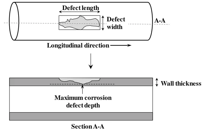
geometry (i.e. corrosion defect depth, length, and width, see Figure 1.2). It should be noted that

Electrolyte (surrounding soil)

Corrosion pit

Ion flow

Cathode area (-)

Anode area (+)

Electron flow, 2e

Oxidation:

2 𝐹 2𝐹

2

−

(18)

MFL tool can differentiate the corrosion defects located on the external and internal surfaces of

the pipe wall and the present study deals only with the corrosion on the external surface of a

pipeline.

Figure 1.2 Schematic illustration of a typical corrosion defect geometry

Despite the immense advancement of the ILI technology, there are still inherent uncertainties

associated with the ILI tool measurements due to imperfections in the tools and associated sizing

algorithms (Al-Amin et al., 2012; Nessim et al., 2008). It is important to quantify these

measurement uncertainties, as they may affect the accuracy of the corrosion defect assessment.

Corrosion defect assessment is a crucial part of corrosion management program of a pipeline,

whereas steps of corrosion management program involve in-line inspection, corrosion defect

assessment and corrosion mitigation (Kishawy and Gabbar 2010). Over the past few decades, the

reliability-based corrosion management programs are increasingly adopted by pipeline operators

as, it can incorporate the uncertainties associated with parameters used in the corrosion assessment.

The parameters associated with the corrosion assessment involves the pipe mechanical and

Longitudinal direction

A-A

Section A-A Defect length

Wall thickness

Maximum corrosion defect depth

(19)

geometric parameters (i.e. pipe diameter, internal pressure, yield strength of the steel pipe etc.) and

the geometric dimension associated with the corrosion defect (i.e. corrosion defect depth, length

etc.). As probabilistic characteristics of the measurement uncertainties associated with ILI tools

are required in the reliability analysis, studies have been conducted in the past decade to facilitate

the use of reliability-based corrosion management programs, such as the development of

probabilistic corrosion defect depth growth models (Al-Amin & Zhou, 2013; Maes et al., 2009;

Zhang & Zhou, 2013) and corrosion defect depth measurement error models (Caleyo et al. 2007;

Nessim et al. 2008; Al-Amin et al. 2012) based on ILI data.

Furthermore, oil and gas transmission pipelines, which are often operated at high internal

pressures, may fail by burst due to the reduced pipe wall thickness caused by metal loss corrosion.

A key component of reliability based corrosion management program is to predict the probability

of the internal pressure of a pipeline exceeding the burst pressure capacity of a corroding pipeline

over a period of time (Zhang and Zhou 2014). There are several empirical burst pressure capacity

models currently used in practice, e.g. the B31G and B31G Modified models (Kiefner and Vieth

1989), Det Norske Veritas (DNV) model (DNV-RP-F101 2010a), the Canadian Standards

Association (CSA) model (CSA 2015), and PCORRC and RSTRENG models (Zhou and Huang

2012) with varying degrees of predictive accuracy. Zhou and Huang (2012) quantified the model

errors associated with the empirical burst pressure capacity models. Furthermore, several

researchers (Ahammed & Melchers, 1996; Amirat et al., 2008; Zhou, 2010) also worked on the

methodologies to evaluate the reliability of corroding pipelines. However, there still exist

knowledge gaps and unaddressed issues that limit the application of the reliability-based

(20)

Burst pressure capacity models such as, the B31G, B31G Modified models, DNV model

uses the simple geometric dimensions of a corrosion defect (i.e. corrosion defect length and

maximum defect depth). On the other hand, the burst pressure capacity models such as RSTRENG

and CSA use the detail geometric corrosion dimensions derived from the river-bottom profile of a

corrosion defect, whereas the river-bottom profile referred to the two-dimensional projection of a

three dimensional corrosion defect. According to Zhou and Huang (2012), the RSTRENG and

CSA models are considered the most accurate burst capacity models compared with the other

empirical models available. However, these models (i.e. RTSRENG and CSA models) are not

easily applicable to corrosion defect assessments, as the required detail geometric characterizations

of corrosion defects (derived from the river-bottom profile of a corrosion defect), are not always

available from the ILI data.

Typically, the burst pressure at a corrosion defect is a function of the corrosion defect depth

and length, along with the other physical and mechanical parameters of the pipeline. Measurement

error models for ILI-measured maximum defect depth have been investigated by several

researchers (e.g. Al-Amin et al. 2012; Caleyo et al. 2007; Nessim et al. 2008); on the other hand,

the measurement error for the ILI-measured defect length has not been reported in the literature.

Ellinger and Moreno (2016) pointed out a poor correlation between the ILI-reported defect lengths

and corresponding field-measured defect lengths, which is largely due to the existence of

clustering errors. In this study, the clustering error referred to the phenomena introduced during

the ILI by erroneously including or excluding multiple or a single corrosion anomaly in or from a

corrosion cluster. In cases where ILI tools do provide defect geometric characterization in addition

(21)

measurement errors associated with the ILI-reported detailed defect geometry within the context

of the involvement of such geometry in the burst pressure prediction model such as RSTRENG.

Objective and Research Significance

The research conducted in this thesis is financially supported by Natural Sciences and

Engineering Research Council (NSERC) of Canada and TransCanada Ltd. The objective of this

research is summarized as follows:

1) Evaluate statistics of the detailed geometric defect profile to facilitate the use of RSTRENG

(Remaining Strength of Corroded Pipe) and CSA (Canadian standards association) burst pressure

capacity models in reliability analysis of corroded pipelines

2) Develop measurement error models associated with the corrosion defect length, and

measurements associated with the effective portion of a defect, reported by ILI

3) Investigate implication of measurement error models for corrosion defect length and

measurement associated with effective portion of a corrosion defect in the system reliability

analysis.

It is expected that the outcome of this research will facilitate in accurately predicting the

reliability-based assessment of corroded pipelines as well as the pipeline integrity management

program.

Scope of the Study

This thesis consists of four main topics that are presented in Chapters 2 to 5, respectively.

(22)

pressure capacity models in the reliability analysis of corroded pipelines. The use of the CSA and

RSTRENG burst pressure capacity models is desirable in the reliability analysis of corroded

pipelines because they incorporate detailed defect geometric information and have relatively small

model uncertainties. Since the detailed defect geometric information is not always available from

ILI of corroded pipelines, this study facilitates the use of CSA and RSTRENG models in the

reliability analysis by deriving probabilistic characteristics of parameters that relate the detailed

defect geometry to its simplified characterizing parameters based on the high-resolution geometric

data for a large set of external metal-loss corrosion defects identified on an in-service pipeline in

Alberta, Canada.

Chapter 3 presents a framework to quantify the measurement error associated with lengths

of corrosion defects on oil and gas pipelines reported by ILI tools based on a relatively large set

of ILI-reported and field-measured defect data collected from different in-service pipelines in

Canada. A log-logistic model is proposed to quantify the likelihood of a given ILI-reported defect

being a Type I defect (without cluster error) or a Type II defect (with clustering error). The

measurement error associated with the ILI-reported length of the defect is quantified as the average

of those associated with the Type I and Type II defects, weighted by the corresponding

probabilities obtained from the log-logistic model.

Chapter 4 presents the quantification of measurement error associated with the effective

portions of a corrosion defect in an oil and gas pipe joint reported by ILI tools based on ILI and

field measured corrosion defect data of several pipelines currently in service in Canada. The study

specifically quantifies the measurement of effective length and effective depth of a corrosion

(23)

associated with the ILI data into the proposed measurement error for effective length and effective

of a corrosion defect. Consequently, the measurement error model quantified in this study will

enable the use of RSRENG model in corrosion assessment, if ILI-reported defect profiles are

available.

Chapter 5 presents the sensitivity of system reliability of corroded pipe joints to the proposed

measurement error model for ILI measured corrosion defect length and measurement error model

for ILI measured dimension for effective portion of a corrosion defect. The system reliability of a

corroded pipelines is compared with the ILI vendors provided measurement errors for corrosion

defects to the proposed measurement error models. A pipe joint that is a part of a pipeline currently

in service in Canada is used as a case study.

Thesis Format

This thesis is prepared as an Integrated-Article Format as specified by the School of Graduate

and Postdoctoral Studies at Western University, London, Ontario, Canada. A total of 6 chapters

are included in this thesis. Chapter 1 presents a brief introduction with background, objective, and

scope of the study. Chapter 2 to 5 consists of the main body of the thesis, each chapter addresses

an individual topic and the key part of the published papers and submitted manuscripts. Finally,

the last Chapter of this thesis consists of conclusion of the thesis and the future work.

Reference

Ahammed, M., and Melchers, R. E. (1996). “Reliability estimation of pressurised pipelines subject

to localised corrosion defects.” International Journal of Pressure Vessels and Piping, 69(3),

(24)

Al-Amin, M., and Zhou, W. (2013). “Evaluating the system reliability of corroding pipelines based

on inspection data.” Structure and Infrastructure Engineering, 10(9), 1161–1175.

Al-Amin, M., Zhou, W., Zhang, S., Kariyawasam, S., and Wang, H. (2012). “Bayesian Model for

Calibration of ILI Tools.” 9th International Pipeline Conference, IPC2012-90491, Calgary,

Alberta, Canada, September 24–28, 201–208.

Alamilla, J. L., Espinosa-Medina, M. A., and Sosa, E. (2009). “Modelling steel corrosion damage

in soil environment.” Corrosion Science, 51(11), 2628–2638.

Amirat, A., Benmoussat, A., and Chaoui, K. (2008). “Reliability assessment of underground

pipelines under active corrosion defects.” 1st African InterQuadrennial ICF Conference on

Damane and Fracture Mechanics-Failure Analysis of Engineering Materials and Structures,

Algiers, Algeria, 83–92.

Caleyo, F., Alfonso, L., Espina-Hernández, J. H., and Hallen, J. M. (2007). “Criteria for

performance assessment and calibration of in-line inspections of oil and gas pipelines.”

Measurement Science and Technology, 18(7), 1787–1799.

CSA. (2015). “CSA Z662: Oil and gas pipeline systems.” Canadian Standard Association,

Mississauga, Ontario, Canada.

Davis, J. R. (2000). Corrosion: Understanding the basics. ASM International, Ohio, USA.

DNV-RP-F101. (2010). Recommended practice: Corroded pipelines. Det Norske Veritas, Hovik.

Ellinger, M. A., and Moreno, P. J. (2016). “ILI-to-Field Data Comparisons - What Accuracy Can

(25)

2016, Calgary, Alberta, Canada, 1–8.

Hopkins, P. (2014). “Assessing the significance of corrosion in onshore oil and gas pipelines.”

Underground pipeline corrosion, Detection, analysis and prevention, M. E. Orazem, ed.,

Woodhead Publishing, UK, 62–84.

Kiefner, J. F., and Vieth, P. H. (1989). A modified criterion for evaluating the remaining strength

of corroded pipe. PR 3-805, American Gas Association, Washing- ton, D.C.

Kishawy, H. A., and Gabbar, H. A. (2010). “Review of pipeline integrity management practices.”

International Journal of Pressure Vessels and Piping, 87(7), 373–380.

Maes, M. A., Faber, M. H., and Dann, M. R. (2009). “Hierarchical modeling of pipeline defect

growth subject to ILI uncertainty.” ASME 28th International Conference on Ocean, Offshore,

and Archtic Engineering, OMAE2009-79470, Honolulu, Hawaii, USA.

Miran, S. A., Huang, Q., and Castaneda, H. (2016). “Time-Dependent Reliability Analysis of

Corroded Buried Pipelines Considering External Defects.” Journal of Infrastructure Systems,

22(3), 04016019.

Nessim, M., Dawson, J., Mora, R., and Hassanein, S. (2008). “Obtaining Corrosion Growth Rates

From Repeat In-Line Inspection Runs and Dealing With the Measurement Uncertainties.” 7th

International Pipeline Conference, ASME, Calgary, Alberta, Canada, 593–600.

NRCan. (2016). “Pipelines Across Canada.”

<https://www.nrcan.gc.ca/energy/infrastructure/18856> (Sep. 16, 2018).

(26)

inspection (ILI), and corrosion growth rate models.” International Journal of Pressure

Vessels and Piping, 149(2017), 43–54.

Zhang, S., and Zhou, W. (2013). “System reliability of corroding pipelines considering stochastic

process-based models for defect growth and internal pressure.” International Journal of

Pressure Vessels and Piping, Elsevier Ltd, 111–112, 120–130.

Zhang, S., and Zhou, W. (2014). “An Efficient methodology for the reliability analysis of

corroding pipelines.” Journal of Pressure Vessel Technology, 136(4), 041701.

Zhou, W. (2010). “System reliability of corroding pipelines.” International Journal of Pressure

Vessels and Piping, 87(10), 587–595.

Zhou, W., and Huang, G. X. (2012). “Model error assessments of burst capacity models for

corroded pipelines.” International Journal of Pressure Vessels and Piping, 99–100(2012), 1–

(27)

2

Evaluation of Statistics of Metal-loss Corrosion

Defect Profile to Facilitate Reliability Analysis of

Corroded Pipelines

Introduction

The structural integrity of oil and gas pipelines may be compromised by metal loss corrosion

defects. Pipeline operators commonly employ high-resolution inline inspection (ILI) tools to

detect, locate, and size corrosion defects. Over the last decade or so, the reliability-based corrosion

management program is being increasingly used (Cosham and Hopkins 2002; Stephens 2006;

Stephens and Nessim 2006; Zhou et al. 2015) as it provides an effective framework to handle the

uncertainties involved in the pipeline corrosion management. A crucial component of such a

program is to predict the probability of burst of the corroded pipeline, i.e. the probability of the

pipeline operating pressure exceeding its burst pressure capacity. Several semi-empirical burst

capacity models for corroded pipelines are widely used in practice, for example, the American

Society of Mechanical Engineers (ASME) B31G and B31G Modified models, the DNV and CSA

models that are recommended in Det Norske Veritas (DNV) OS-F101 and Canadian Standards

Association (CSA) Z662-15 respectively, the PCORRC and RSTRENG models (Cronin 2000;

Zhou and Huang 2012). These models generally predict the burst capacity as functions of the defect

depth and length, pipe geometry (i.e. diameter and wall thickness), and material strength (e.g.,

yield strength, tensile strength, or flow stress). The geometry of a typical metal-loss corrosion

defect on a pipeline is illustrated in Figure 1. The length and depth of the defect are measured in

the longitudinal and through-wall thickness directions, respectively, of the pipeline. Based on the

defect geometry employed, the aforementioned burst capacity models can be classified as Type I

(28)

require simplified characterizing parameters for the defect geometry, namely the maximum defect

depth and length (Figure 2.1), to predict the burst pressure. On the other hand, Type II models,

which include the RSTRENG and CSA models, require a so-called river-bottom defect profile

(Figure 2.1) to predict the burst pressure. In particular, the RSTRENG model (Kiefner and Vieth

1989) involves identifying the effective portion of the defect profile that leads to the lowest

predicted burst pressure, whereas the CSA model (CSA 2015) involves evaluating the average

depth from the defect profile.

The burst capacity models are not perfectly accurate and therefore involve model errors.

Zhou and Huang (2012) evaluated model errors associated with the aforementioned burst capacity

models based on a large database of full-scale burst tests of corroded pipes reported in the

literature. According to their report, Type II models are markedly more accurate than Type I

models; this is expected since the former incorporate more information about the defect geometry

than the latter in predicting the burst capacity. It follows that Type II models are more

advantageous than Type I models in the reliability-based corrosion defect assessment. However,

while ILI tools always report the maximum depth and length for a given detected corrosion defect,

they quite often do not provide its detailed defect profile. To facilitate the use of Type II models

in the reliability analysis, it is therefore desirable to develop statistical relationships between the

defect profile and its simplified characterizing parameters.

Reports of statistical relationships between the defect profile and simplified characterizing

parameters are scarce, if any, in the literature. The Canadian oil and gas pipeline standard CSA

Z662-15 (CSA 2015) recommends that the ratio of the maximum to average defect depths be

(29)

variation (COV) of 50% and a lower bound of unity. As indicated in Z662-15, this distribution is

derived based on the geometry of defects on the full-scale corroded pipe sections reported by

Kiefner and Vieth (1989). It is however unclear how many data points are used to derive the

distribution (a total of 98 corroded pipe sections are reported by Kiefner and Vieth (1989)) and

how well the distribution fits the data. Furthermore, to the best of our knowledge, relationships

between the effective portion of the defect profile and maximum defect depth or length are

unavailable in the literature. It is therefore necessary to fill the above-described knowledge gap to

improve the pipeline corrosion management practice.

Figure 2.1 Typical defect characterization

The objective of the work reported in this paper is to collect the geometric data of a large

number of naturally-occurring corrosion defects on pipelines and employ the collected data to

derive statistical relationships between the defect profile and its simplified characterizing

parameters. To this end, defect geometric data for 470 external corrosion defects measured by laser

Effective portion of the defect Contour of “River bottom” path of the defect

Effective defect length,

Defect length,

Defect width,

Average defect depth,

Maximum defect depth, 𝒙

Effective area,

(30)

scanning devices are collected from an in-service natural gas pipeline located in Alberta, Canada.

Statistical analyses are then carried out to derive the probability distributions of the

average-to-maximum depth ratios, ratio between the average depth of the effective defect profile and

maximum depth of the overall defect profile, and ratio between the length of the effective defect

profile and length of the overall defect profile. The implications of the obtained results are then

investigated by using the B31G Modified, CSA and RSTRENG models to evaluate the

probabilities of burst of several representative pipelines containing corrosion defects with

ILI-reported defect dimensions.

The rest of the paper is organized as follows. Section 2.2 briefly reviews the B31G Modified,

RSTRENG and CSA models. Section 2.3 describes the defect geometric data collected from the

gas pipeline in Alberta and statistical analyses carried out to develop the relationship between the

defect profile and its simplified characterizing parameters. The implications of the obtained results

for the reliability analysis of corroded pipelines are presented in Section 2.4, followed by

concluding remarks in Section 2.5.

Burst Pressure Capacity Models

The CSA and RSTRENG models are both Type II burst capacity models and reviewed in

this section. The B31G Modified model is a representative Type I burst capacity model and serves

as a basis for the CSA and RSTRENG models; therefore, the B31G Modified model is also

reviewed. Let Pb denote the burst pressure capacity of a pipeline at a given corrosion defect. Then

Pb can be evaluated using the B31G Modified, CSA and RSTRNG models, respectively, as

(31)

B31G Modified model

𝑃𝑏 =

2𝑡(𝜎𝑦 68.95)

𝐷 [

1 −0.85𝑑𝑚𝑎𝑥

𝑡 1 −0.85𝑑𝑚𝑎𝑥

𝑀𝑡

], 𝑑𝑚𝑎𝑥

𝑡 ≤ 0.8

(2.1)

CSA model

𝑃_𝑏 = 𝜉₂2𝑡𝜎𝑓 𝐷

1 −𝑑𝑎𝑣𝑔_𝑡

1 −𝑑_𝑡𝑀𝑎𝑣𝑔

(2.2)

𝜎𝑓 = {

1.15𝜎𝑦 𝜎𝑦 ≤ 2 1𝑀𝑃𝑎

0.9𝜎𝑢 𝜎𝑦 > 2 1𝑀𝑃𝑎

(2.3)

𝑀 =

{

√1 0.6275 𝑙2

𝐷𝑡− 0.003375 𝑙4

(𝐷𝑡)2,

𝑙2

𝐷𝑡≤ 50

3.3 0.032 𝑙2 𝐷𝑡,

𝑙2

𝐷𝑡> 50

(2.4)

RSTRENG model

𝑃_𝑏 = 𝑚𝑖𝑛{𝑃_𝑏𝑗} 𝑗 = 1, 2, … , 𝑛 (2.5)

𝑃_𝑏𝑗 = 𝜉₃2𝑡(𝜎𝑦 68.95) 𝐷

1 −_𝑙𝐴𝑗

𝑗𝑡

1 −_𝑀𝐴𝑗

𝑗𝑙𝑗𝑡

𝑑𝑚𝑎𝑥

𝑡 ≤ 0.8 𝑗 = 1, 2, … , 𝑛

(2.6)

where, in Eqs. (2.1) through (2.6), dmax, davg and l denote the maximum depth, average depth, and

length of the corrosion defect respectively; D and t are the pipe outside diameter and wall

thickness, respectively; y, u and f are the pipe yield strength, tensile strengths, and so-called

flow stress, respectively; y + 68.95 (MPa) is an empirical equation employed in the B31G

Modified and RSTRENG models to determine f, M is the Folias or bulging factor to account for

(32)

B31G Modified, CSA, and RSTRENG models, respectively. To apply the RSTRENG model, one

needs to generate n sub-defects based on the defect profile, each sub-defect being a contiguous

portion of the overall defect. The area and length of the j-th (j = 1, 2, …, n) sub-defect are denoted

by Aj and lj, respectively, and the corresponding Folias factor Mj is evaluated by replacing l with lj

in Eq. (2.4). The sub-defect that has the lowest burst capacity is defined as the effective portion of

the overall defect, with the corresponding area and length defined as the effective area (Aeff) and

length (leff) of the defect, respectively (see Figure 2.1). It should be clarified that the B31G

Modified, CSA, and RSTRENG models as originally proposed do not include the model errors,

i.e. 𝜉1, 𝜉2 and 𝜉3 respectively. They are included in Eqs. (2.1), (2.2) and (2.6), respectively,

because the model error is a key random variable that must be considered in the reliability analysis

of corroded pipelines.

Statistical Analysis of Defect Geometric Data

Data Description

The corrosion geometric data analyzed in this study are collected from the corrosion

assessment field reports for an in-service natural gas pipeline located in Alberta, Canada. Due

primarily to the deterioration of the coating condition, ILI tools found a significant number of

corrosion defects on the external surface of the pipeline. The assessment reports were prepared by

the contractors retained by the pipeline operator to excavate and repair corroded pipe joints (a

typical pipe joint is about 12 m long) that contained critical defects and were therefore deemed in

need of repair based on fitness-for-service assessments of defects using the relevant ILI

information. The reports reviewed in this study cover a period of 7 years, from 2004 to 2011. For

each of the excavated pipe joints, the repair crew used a high-resolution laser-scanning device to

(33)

into several segments [see Figure 2.2(a)]. Figure 2.2(b) depicts the laser-scanned image for one

arbitrarily selected defect in the pipe segment shown in Figure 2.2(a). The RSTRENG model was

employed afterward to evaluate the burst capacities at the defects based on the laser-scanned defect

geometry. The reports document key geometric data for the defects, including dmax, davg, l, Aeff, and

leff, obtained from the laser scanning device and RSTRENG assessments. It must be emphasized

that although all the excavated pipe joints contained critical corrosion defects, the laser scan

captured the geometry of all the defects (i.e. critical as well as non-critical defects) on a given

joint. Therefore, the defect geometric data collected from the assessment reports are considered

representative of the entire defect population as opposed to the population of critical defects only.

(a)

(34)

(b)

Figure 2.2 (a) Laser scan picture of a segment of a pipe joint, and (b) Laser scan picture of

a corrosion defect of the corresponding pipe segment

By reviewing the assessment reports, the geometric data for a total of 470 corrosion defects

were collected. The values of dmax, davg, and l for these defects range from 9.9 to 84.6% of the pipe

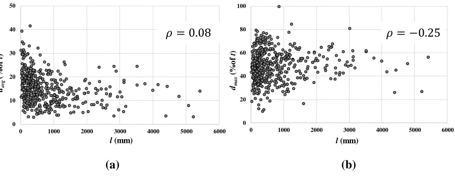
wall thickness (t), from 2.9 to 41.5%t, and from 16 to 5420 mm, respectively. Figure 2.3 depicts

the relationships between dmax andl, and between davg and l for the 470 defects. The Pearson

correlation coefficients (i.e. ) evaluated from the data are shown in the corresponding panels of

the figure. The figure suggests that there are negligible correlations between dmax andl, and davg

and l.

(35)

(a) (b)

Figure 2.3. Relationships between (a) dmax andl, and (b) davg and l

Statistical Analysis

For the statistical analyses, the following quantities are defined.

𝜇 = 𝑑𝑎𝑣𝑔

𝑑𝑚𝑎𝑥 (2.7a)

𝜆 =𝑙𝑒𝑓𝑓

𝑙 (2.7b)

𝜂 = 𝐴𝑒𝑓𝑓

𝑙𝑒𝑓𝑓𝑑𝑚𝑎𝑥 (2.7c)

It follows from Eq. (2.7) that  (0 <  ≤ 1) is the average-to-maximum depth ratio;  (0 <  ≤ 1)

is the ratio between the effective length and total length of the defect, and  (0 <  ≤ 1) is the ratio

between the average depth (i.e. Aeff/leff) of the effective portion of the defect and dmax. Given dmax,

l, ,  and , one can evaluate davg = dmax, leff = l and Aeff = ldmax. Figure 2.4 depicts the

relationships between  and dmax,  and l,  and dmax,  and dmax,  and l,  and l, and  and ,

with the corresponding Pearson correlation coefficients given in the corresponding panels of the 0

10 20 30 40 50

0 1000 2000 3000 4000 5000 6000

dav

g

(%

o

f

t)

l (mm)

0 20 40 60 80 100

0 1000 2000 3000 4000 5000 6000

dm

ax

(%

o

f

t)

l (mm)

(36)

figure. The figure suggests that there are negligible correlations between  and dmax,  and l,  and

dmax,  and dmax,  and l, and  and , and a relatively strong correlation between  and l.

(a) (b)

(c) (d)

0 0.2 0.4 0.6 0.8 1

0 20 40 60 80 100

μ

dmax (%t)

0 0.2 0.4 0.6 0.8 1

0 1000 2000 3000 4000 5000 6000

μ

l (mm)

0 0.2 0.4 0.6 0.8 1

0 20 40 60 80 100

λ

dmax (%t)

0 0.2 0.4 0.6 0.8 1

0 20 40 60 80 100

η

dmax (%t)

𝜌 = −0.22 𝜌 = −0.31

(37)

(e) (f)

(g)

Figure 2.4. Relationship between (a)  and dmax ,(b)  and l, (c)  and dmax, (d)  and dmax,

(e)  and l, (f)  and l, and (g)  and 

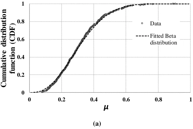
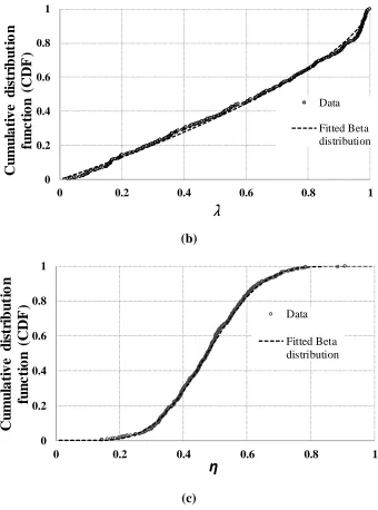
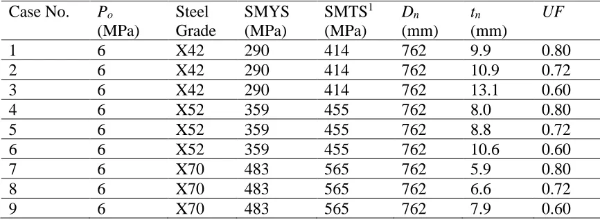
Figure 2.5 depicts the empirical cumulative distribution functions (CDF) of ,  and 

obtained from the 470 data points, whereby the empirical CDF for the i-th (i = 1, 2, …, 470) data

point equals i/471, as well as CDF of the corresponding best-fit distributions. Given that ,  and

 are all bounded between zero and unity, the standard beta distribution is a natural choice to fit

the data. The Kolmogorov-Smirnov test (Ang and Tang 1975) confirms that the standard beta

distribution is the best fit distribution for ,  and  compared with the gamma, lognormal, and

0 0.2 0.4 0.6 0.8 1

0 1000 2000 3000 4000 5000 6000

λ

l (mm)

0 0.2 0.4 0.6 0.8 1

0 1000 2000 3000 4000 5000 6000

η

l (mm)

0 0.2 0.4 0.6 0.8 1

η

λ

𝜌 = −0.67 _{𝜌 = −0.13}

(38)

exponential distributions. The means, coefficients of variation (COV) and corresponding

distribution parameters q and r for ,  and  are summarized in Table 2.1. The probability density

function (PDF) of a standard beta-distributed variate Y, fY(y), is given by

𝑓_𝑌(𝑦) =_{𝐵(𝑞,𝑟)}1 𝑦𝑞−1_{(1 − 𝑦)}𝑟−1_{(0 ≤ y ≤ 1)} _(2.8)

𝐵(𝑞, 𝑟) =Γ(𝑞)Γ(𝑟)_{Γ(𝑞 𝑟)} (2.9)

where B(q, r) is the beta function; (•) is the gamma function, and the mean and COV of Y are

given by q/(q+r) and √_{𝑞(𝑞 𝑟 1)}𝑟 , respectively. Table 2.1 indicates that for the 470 defects analyzed,

davg is on average 32% of dmax; leff is on average 61% of l, and Aeff/leff is on average 48% of dmax.

Furthermore, ,  and  all have relatively high variability with COV values ranging from about

25 to 50%.

It is noted that the probabilistic characteristics of ,  and  obtained in the present study

are based on the corrosion defect data collected from a single in-service pipeline and may not be

applicable to other pipelines, if the morphology of the corrosion defect is largely influenced by

relevant pipe attributes such as the coating properties, as well as properties of the surrounding

soils. The potential dependence of the corrosion morphology on the coating and soil properties is

(39)

Table 2.1 Basic statistics of μ, λ and η

Parameter Mean COV Best-fit distribution

Beta distribution parameters

q r

 0.32 44% Beta

(Lower bound = 0; Upper bound = 1)

3.242 6.912

 0.61 49% 1.025 0.655

 0.48 27% 6.795 7.444

(a) 0 0.2 0.4 0.6 0.8 1

0 0.2 0.4 0.6 0.8 1

(40)

(b)

(c)

Figure 2.5. Cumulative probability plots for (a) 𝝁, (b) 𝝀, and (c) 𝜼

Practical Implications

Probability of Burst of Corroded Pipeline

The practical implications of the parameters ,  and  described in Section 2.3 for the

evaluation of the probability of burst of corroded pipelines are discussed in this section. The limit

0 0.2 0.4 0.6 0.8 1

C u m u la ti v e d is tr ib u ti o n fu n c ti o n (CD F )

λ

Data Fitted Beta distribution 0 0.2 0.4 0.6 0.8 1

0 0.2 0.4 0.6 0.8 1

(41)

state function, g, for the evaluation of the probability of burst of a pipeline containing a corrosion

defect is expressed as,

𝑔 = 𝑃_𝑏− 𝑝 (2.10)

where p is the pipeline operating pressure, Pb is the pipe burst pressure capacity at the defect, and

g ≤ 0 represents burst (i.e. failure).

The probability of failure (burst), Pf, is given by,

𝑃_𝑓 = ∫_𝑔≤0𝑓_𝑿(𝒙)𝑑𝒙 (2.11)

where 𝑓_𝑿(𝒙) denotes the joint PDF of the vector of n random variables, X = [X1, X2, …, Xn]T (T

denotes transposition), that are involved in the limit state function, including the defect geometric

dimensions, pipe yield or tensile strength, model error and pipeline operating pressure. The

first-order reliability method (FORM) (Melchers 1999a) is employed in this study to evaluate the

integral in Eq. (2.11). It follows that Pf is approximated by (-), where (•) is the CDF of the

standard normal distribution function, and  is the reliability index representing the shortest

distance between the origin and limit state surface in the standard normal space. The value of  is

obtained through a constrained optimization analysis in the FORM with the constraint being g ≤ 0

in the standard normal space.

To carry out the FORM analysis, the vector of random variables X needs to be transformed

to a vector of n independent standard normal variates U = [U1, U2, …, Un]T. If the individual

random variables in X are mutually independent, the transformation can be straightforwardly

(42)

−_{(•) is the inverse of the standard normal distribution function, and F}

i(xi) is the CDF of Xi (Der

Kiureghian 2005). If the individual random variables in X are correlated, the Nataf transformation

(Der Kiureghian 2005) is commonly used. That is, X is first transformed to a set of n correlated

standard normal variates Z = [Z1, Z2, …, Zn]T through the inverse normal transformation, and Z is

then transformed to U through U = L-1Z, where L is the lower-triangular matrix obtained from the

Cholesky decomposition of the correlation matrix associated with Z. Empirical equations have

been developed by Der Kiureghian and Liu (Der Kiureghian and Liu 1986) to evaluate the

correlation coefficient between Zi and Zk given the correlation coefficient between Xi and Xk (i, k

= 1, 2, …, n) for various marginal distributions. The difference between the two correlation

coefficients is in general small; therefore, the former can be considered to approximately equal the

latter. Note that the reliability analysis carried out in the present study corresponds to the defect

assessment to identify critical defects to be repaired immediately after ILI. Therefore, the analysis

does not consider the growth of corrosion defects over time or fluctuation of the pipeline operating

pressure with time; in other words, the time-invariant reliability analysis is carried out.

Analysis Cases and Probabilistic Characteristics of Input

Parameters

The analysis considers nine representative natural gas pipelines corresponding to a nominal

pipe outside diameter of 762 mm, three pipe steel grades (X42, X52 and X70), and a maximum

operating pressure (MOP) of 6.0 MPa. The nominal pipe wall thicknesses (tn) of the nine analysis

cases are determined as follows:

(43)

where Po denotes MOP; SMYS is the specified minimum yield strength of the pipe steel; Dn

denotes the nominal pipe outside diameter, and UF (UF < 1) is the utilization factor (i.e. safety

factor) that limits the pipe hoop stress due to MOP to a fraction of SMYS. Three values of UF,

namely 0.80, 0.72 and 0.60, that are typical for natural gas transmission pipelines in Canada are

considered in the analysis. Table 2.2 summarizes the attributes of the nine pipeline cases

considered in the analysis.

Table 2.2 Attributes of representative pipelines considered in the analysis

Case No. Po

(MPa)

Steel Grade

SMYS (MPa)

SMTS1

(MPa)

Dn

(mm) tn

(mm)

UF

1 6 X42 290 414 762 9.9 0.80

2 6 X42 290 414 762 10.9 0.72

3 6 X42 290 414 762 13.1 0.60

4 6 X52 359 455 762 8.0 0.80

5 6 X52 359 455 762 8.8 0.72

6 6 X52 359 455 762 10.6 0.60

7 6 X70 483 565 762 5.9 0.80

8 6 X70 483 565 762 6.6 0.72

9 6 X70 483 565 762 7.9 0.60

1_{SMTS denotes the specified minimum tensile strengths}

For each of the analysis cases, it is assumed that the pipeline contains a corrosion defect

with the ILI-reported maximum depth (dmax-ILI) and length (lILI). Four

𝑑max−𝐼𝐿𝐼

𝑡𝑛 values (0.3, 0.4, 0.5

and 0.6), and five 𝑙_𝐼𝐿𝐼 values (50, 150, 250, 350, and 500 mm) are considered such that the failure

probability of a given pipeline is analyzed for 20 different sets of dmax-ILI and lILI. For each set of

dmax-ILI and lILI, three reliability analyses are carried out by employing the B31G Modified, CSA

and RSTRENG models, respectively. The analysis employing the B31G Modified model involves

dmax and l, which can be evaluated from dmax-ILI and lILI, respectively, by considering the

(44)

analyses employing the CSA and RSTRENG models, ,  and  are used to evaluate davg, leff and

Aeff from dmax and l, i.e. davg = dmax for the CSA model, and leff = l and Aeff = ldmax for the

RSTRENG model. The probabilistic characteristics of parameters ,  and  are given in Table

2.1. Based on the results shown in Figure 2.4, , , , dmax, and l are considered mutually

independent except that λ and l are considered correlated with the corresponding correlation

coefficient equal to -0.67 in the reliability analysis. This correlation coefficient is assumed to be

the same as that in the correlated normal space in the FORM analysis. To investigate the sensitivity

of the analysis results to the correlation between λ and l, FORM analyses are also carried out by

assuming λ and l to be independent.

Table 2.3 summarizes the probabilistic characteristics of the random variables associated

with the pipe geometric and material properties, and dmax and l. It is assumed that all the random

variables in the table are mutually independent. Statistical information provided in Annex O of

CSA Z662-15 (CSA 2015b) indicates that t/tn generally follows a normal distribution with the

mean ranging from 1.0 to 1.01 and COV ranging from 1.0 to 1.7%. Hence, t/tn is assigned a normal

distribution with the mean equal to unity and COV equal to 1.5% in the present study. The actual

pipe outside diameter typically equals the nominal outside diameter with negligible uncertainty

(CSA 2015b). It is also indicated in CSA Z662-15 that both normal and lognormal distributions

are adequate to characterize y/SMYS and u/SMTS, with the mean values close to 1.1 and COV

values ranging from 3 to 3.5%. Jiao et al.(Jiao et al. 1995) suggested that 𝑃 𝑃⁄ _𝑜 (i.e. ratio of the

maximum annual pressure and MOP) follows a Gumbel distribution with a mean between 1.03

and 1.07 and a COV between 1 and 2%. Hence, the present study considers 𝑃 𝑃⁄ 𝑜 follows a Gumbel

(45)

the model errors associated with various burst pressure capacity models based on 150 full-scale

burst tests of pipe segments containing single isolated natural corrosion defects. The probabilistic

characteristics of model errors associated with the B31G Modified (1), CSA (2) and RSTRENG

(3) models, respectively, as shown in Table 2.3 are based on the results reported by Zhou and

Huang (2012). The characteristics of the three model errors suggest that the CSA and RSTRENG

models are markedly more accurate than the B31G Modified model.

The ILI-reported maximum defect depth and defect length are assumed to be related to the

actual maximum defect depth and defect length, respectively, by additive measurement errors

(DNV-RP-F101 2010b; Zhou and Nessim 2011) as follows:

𝑑_{max−𝐼𝐿𝐼} = 𝑑_𝑚𝑎𝑥 𝜀_𝑑 (2.13)

𝑙𝐼𝐿𝐼 = 𝑙 𝜀𝑙 (2.14)

where 𝜀_𝑑 and 𝜀_𝑙 are the measurement errors associated with dmax-ILI and lILI, respectively. It is

commonly assumed in the literature (Caleyo et al. 2007; DNV-RP-F101 2010b; Zhou and Nessim

2011; Zhou et al. 2015) that 𝜀_𝑑 and 𝜀_𝑙 are normally-distributed random variables with a zero mean.

The standard deviations of 𝜀_𝑑 and 𝜀_𝑙 can be derived from ILI tool specifications (Stephens and

Nessim 2006). For example, typical ILI tool specifications state that dmax-ILI is within dmax±10%tn

80% of the time, and that lILI is within l±10 mm 80% of the time (Stephens and Nessim 2006). It

(46)

Table 2.3 Probabilistic characteristics of random variables in the reliability analysis

Variable Distribution Mean COV (%) Source

t/tn Normal 1.0 1.5

CSA (2015)

y/SMYS Lognormal 1.1 3.5

u/SMTS Lognormal 1.09 3.0

D/Dn Deterministic 1.0 0

P/Po Gumbel 1.0 3.0 Jiao et al. (1995)

d (%tn) Normal 0 7.8* Stephens and Nessim

(2006)

l (mm) Normal 0 7.8*

 Gumbel 1.297 25.8

Zhou and Huang (2012)

 Lognormal 1.103 17.2

 Normal 1.067 16.5

*_{The values are standard deviation.}

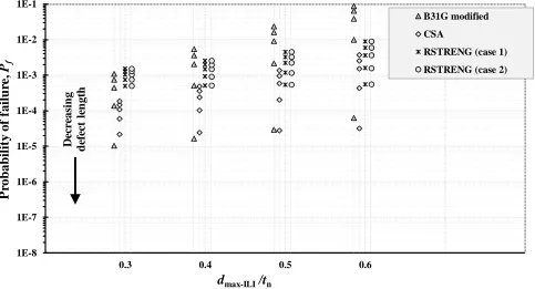
Analysis Results and Discussion

The results of the reliability analysis are shown in Figure 2.6. In this figure, the probability

of failure (i.e. burst), Pf, are plotted against

𝑡𝑛 (i.e. 0.3, 0.4, 0.5, and 0.6). Nine cases with

different combinations of the steel grade (X42, X52, and X70) and 𝑈𝐹 (0.72, 0.8, and 0.6) are

shown in Figures 2.6(a)-(i). Each of the 𝑑max−𝐼𝐿𝐼

𝑡𝑛 values on the horizontal axis corresponds to four

vertical lines representing results of the reliability analysis based on the B31G Modified model,

CSA model, RSTRENG model with independent λ and l (case 1), and RSTRENG model with

correlated λ and l (case 2), respectively. The five points on a given vertical line in the order of the

highest to the lowest points correspond to lILI of 500, 350, 250, 150, and 50 mm, respectively. In

other words, the greater is the ILI-reported defect length, the higher is the failure probability with

all the other parameters being the same.

Figures 2.6(a)-(i) show that Pf corresponding to the B31G Modified model increases

(47)

shown in Figure 2.6(a), when the defect length increases from 50 to 150 mm with 𝑑max−𝐼𝐿𝐼_𝑡

𝑛 = 0.3,

Pf increases approximately by 500%, 100%, and 40%, respectively, corresponding to the B31G

Modified, CSA, and RSTRENG models (for both cases 1 and 2). As 𝑑max−𝐼𝐿𝐼_𝑡

𝑛 increases from 0.4 to

0.5 with lILI = 150 mm, Pf increases by approximately 160%, 60%, and 20%, respectively,

corresponding to the B31G Modified, CSA, and RSTRENG (both cases 1 and 2), respectively.

These results suggest that the Pf corresponding to the B31G Modified model is highly sensitive to

the change in the defect size, compared with those corresponding to the CSA and RSTRENG

models. For a given defect with relatively large 𝑑max−𝐼𝐿𝐼_𝑡

𝑛 and lILI (e.g. for the defect with

𝑡𝑛 =

0.6 and lILI = 500 mm shown in Figure 2.6(a)), Pf corresponding to the B31G Modified model can

be order-of-magnitude higher than those corresponding to the CSA and RSTRENG models.

Figure 2.6 also indicates that Pf corresponding to the RSTRENG model varies in a more

gradual fashion in response to the change in the defect sizes compared with those corresponding

to the B31G Modified and CSA models. This is likely attributed to that the use of  and , both of

which are less than unity, for converting dmax and l to leff and Aeff makes the calculated failure

probability less sensitive to the changes in 𝑑max−𝐼𝐿𝐼_𝑡

𝑛 and lILI. The values of Pf corresponding to the

two cases of RSTRENG models are practically identical for all the analysis cases considered. This

suggests that the correlation between  and l has virtually no effects on Pf. It follows that such a

correlation can be ignored, and  and l can be simply considered as independent in the reliability

analysis.

Figure 2.6 suggests that Pf corresponding to the CSA model is sensitive to the steel grade,

Quantification of Uncertainties in Inline Inspection Data for Metal-loss Corrosion on Energy Pipelines and Implications for Reliability Analysis