Linear Analysis of Reduced-Round CubeHash
Tomer Ashur and Orr Dunkelman
Faculty of Mathematics and Computer Science Weizmann Institute of Science
P.O. Box 26 Rehovot 76100, Israel
Abstract. Recent developments in the field of cryptanalysis of hash func-tions has inspired NIST to announce a competition for selecting a new cryp-tographic hash function to join the SHA family of standards. One of the 14 second-round candidates is CubeHash designed by Daniel J. Bernstein. CubeHash is a unique hash function in the sense that it does not iterate a common compression function, and offers a structure which resembles a sponge function, even though it is not exactly a sponge function.
In this paper we analyze reduced-round variants of CubeHash where the adversary controls the full 1024-bit input to reduced-round CubeHash and can observe its full output. We show that linear approximations with high biases exist in reduced-round variants. For example, we present an 11-round linear approximation with bias of 2−235, which allows distinguishing
11-round CubeHash using about 2470
queries. We also discuss the extension of this distinguisher to 12 rounds using message modification techniques. Finally, we present a linear distinguisher for 14-round CubeHash which uses about 2812
queries.
Key words:CubeHash SHA-3 competition, Linear cryptanalysis.
1
Introduction
Recent developments in the field of hash function cryptanalysis [1,18–20] along with new results targeted against commonly used hash functions [6, 11, 26, 27] has urged National Institute of Standards and Technology to announce a competition for the development of a new hash standard, SHA-3 [25].
The National Institute of Standards and Technology has received 64 hash func-tion proposals for the competifunc-tion, out of which 51 met the submission criteria and were accepted to the first round of the competition. Following the first round of analysis, in which the security and performance claims of the submitters were chal-lenged, 14 candidates were selected to the second round of the SHA-3 competition. One of these 14 candidates is CubeHash designed by Daniel J. Bernstein [4].
CubeHash is a family of cryptographic hash functions, parameterized by the performance and security required. CubeHash has an internal state of 1024 bits, which are processed by calling a transformation namedT, a tweakable number of times r, between introductions of new b-byte message blocks (b is also a tunable parameter). At the end, after a final permutation, namely,T repeated 10r times,
hbits of the state are used as an output. By selecting different values of h, b,and
parameters are suggested, where the “normal” security values are r = 16, b = 32 (forh∈ {224,256,384,512}) [5].1
In this paper we analyze the security of several variants of CubeHash against linear cryptanalysis. Our analysis found a linear approximation for 11-round Cube-Hash2
with bias of 1 4·
1 2
233
= 2−235. We limited the analysis to biases of no less than 2−256, as we felt that a hash function offering a 512-bit security (in its strongest variant), should not be assessed with attacks taking more than 2512
queries. One can also extend the 11-round linear approximation into a 12-round distinguisher using simple message modification techniques [27] (or a chosen-plaintext linear cryptanal-ysis [22]).
We note that when removing this restriction, one can find 14-round linear ap-proximations with bias of 2−406. Exploiting this approximation requires querying
T14
about 2812
times, which is outside the security model. At the same time, ifT
or CubeHash are ever used in different settings, this may provide some indication concerning its security.
This paper is organized as follows: In Section 2 we describe CubeHash’s com-pression function. In Section 3 we describe the linear approximations found for CubeHash. In Section 4 we describe how bit fixing can be used to distinguish more rounds than in the approximation. In Section 5 we quickly cover a possible appli-cation of our results. Finally, Section 6 concludes this paper.
2
A Brief Description of CubeHash
As mentioned before, CubeHash is a tweakable hash function, where the shared part of all its variants is the internal state (of 1024 bits), and the use of the same round functionT.
To initialize the hash function, h(the digest size), r the number of times T is iterated between message blocks, andbthe size of the message blocks (in bytes), are loaded into the state. Then, the state is updated using 10rapplications ofT. At this point, the following procedure is repeated with any new message block: theb-byte block is XORed into the 128-byte state, and the state is updated by applying Tr (r times applyingT) to the state. After processing the padded message, the state is XORed with the constant 1, and is processed by applying T10r. The output is composed of the firsth/8 bytes of the state.
The 1024 bits of the internal state are viewed as a sequence of 32 4-byte words
x00000, x00001, . . . , x11111each of which is interpreted in a little-endian form as a
32-bit unsigned integer. The round function T of CubeHash is based on the following ten operations:
1. Add (modulo 232
)x0jklm into x1jklm, for all (j, k, l, m).
2. Rotate x0jklm left by 7 bits, for all (j, k, l, m). 3. Swapx00klm withx01klm, for all (k, l, m).
4. XORx1jklm intox0jklm, for all (j, k, l, m). 5. Swapx1jk0m withx1jk1m, for all (j, k, m).
6. Add (modulo 232
)x0jklm into x1jklm, for all (j, k, l, m).
1
We note that there is a “formal” variant of CubeHash for whichr = 16, b= 1 and h∈ {384,512}.
2
7. Rotate x0jklm left by 11 bits, for all (j, k, l, m). 8. Swapx0j0lm withx0j1lm, for all (j, l, m).
9. XORx1jklm intox0jklm, for all (j, k, l, m). 10. Swapx1jkl0 withx1jkl1, for all (j, k, l).
The structure is represented in a little endian form, i.e.,x00000 is composed of
the four least significant bytes of the state and x11111 is composed of the most
significant four. We note that the only nonlinear operations with respect to GF(2) are the modular additions.
2.1 Previous Results on CubeHash
Following its simple structure, CubeHash has received a lot of cryptanalytic atten-tion. Some of the attacks, such as the ones of [7, 21], can be applied to CubeHash, independent of the actualT (as long as it is invertible). These attacks target the preimage resistance of CubeHash, and exploit the fact that as all components are invertible, and as the adversary can controlb-bytes of the internal state directly, it is possible to find a preimage in about 2512−4b CubeHash computations.
The second type of results, tried to analyze reduced-round variants of CubeHash for collisions. In [2], a collision for CubeHash2/120-512 is given. Collisions for Cube-Hash1/45 and 2/89 are given in [14], and for CubeHash4/48 and CubeHash4/64 are produced by [9, 10]. A more general methodology to obtain such collisions is described in [8], where variants up to CubeHash7/64 are successfully analyzed.
A third type of attacks/observations concerning CubeHash deal with the sym-metric structure ofT. For example, if at the input allx0jklm words are equal, and allx1jklm words are equal (not necessarily equal to the value of the x0jklm), then the same property holds in the output as well. The first analysis of this type of properties is given in the original submission document [4]. In [3], several additional classes of “symmetric” states are observed, and their use is analyzed. Recently, these classes were expanded to include a larger number of states (and structures) in [16]. Despite all the above-mentioned work, CubeHash is still considered secure, as no attack comes close to offer complexity which is significantly better than generic attacks.3
To the best of our knowledge this work is the first one that succeeds to offer some non-trivial property of more than 10 rounds ofT.
3
Linear Approximation of CubeHash
Linear cryptanalysis [24] is a useful cryptanalytic tool in the world of block cipher cryptanalysis. The cryptosystem is linearly approximated (by an expression that holds with some bias), and the adversary gains information concerning the key, by observing sufficient amount of plaintext/ciphertext pairs satisfying the approxima-tion.
In the context of hash functions, linear cryptanalysis has received very little attention, unlike differential cryptanalysis. The reason for that seems that while differential cryptanalysis can be directly used to offer collisions or preimages, lin-ear cryptanalysis seems to be restricted to very rare cases (i.e., where the bias is extremely high).
3
At the same time, the use of linear approximation to assess the security of a hash function can shed some light on whether the underlying components offer the required security. Moreover, linear approximations of the compression function might be useful when discussing MACs built on top of the hash function (suggesting a detectable linear bias in the output).
3.1 Linear Approximation of Addition Modulo 232
CubeHash uses a mixture of XORs, rotations, and additions. While the first two can be easily handled in the linear cryptanalysis framework, the approximation of the modular addition possess several problems, mostly due to the carry chains.
One of the papers studying the cryptographic properties of modular addition is [12] which studies the carry effects on linear approximations. In the paper, Cho and Pieperzyk show that approximating two consecutive bits can overcome some of the inherent problems of carry chains. Namely, ifλis a mask of two consecutive bits (in any position) then:λ·(x+y) =λ(x⊕y) with probability 3/4 (i.e., a bias of 1/4).
We analyzed several cases where λcontains pairs of consecutive bits, e.g., two pairs of consecutive pairs, and even when these pairs appear immediately after each other (i.e., λ is composed of four consecutive bits set to 1). Our analysis shows that with respect to linear cryptanalysis, these pairs can be treated as two separate independent instances. For example, the probability thatλ·(x+y) =λ(x⊕y) for
λwhose four most significant bits are 1, while the rest are 0, is 10/16 (suggesting the expected bias of 2·(1/4)2
= 1/8).
3.2 The Linear Approximation of the Round Function of CubeHash
Our first attempt in understanding the security of CubeHash against linear crypt-analysis was a very simple experiment. We looked at all possible masks which had only one pair of two consecutive bits active, and tried to extend this mask as many rounds as possible in the forward direction. At some point, the resulting mask had a divided pair of bits, i.e., a pair of bits that due to the rotations used in CubeHash were sent one to the LSB of a word, and one to the MSB of a word. Such a mask does no longer fall under the type of masks considered in [12], and our experiments show that such a mask has a very low bias when considering addition.
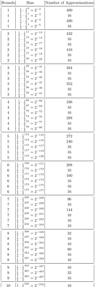
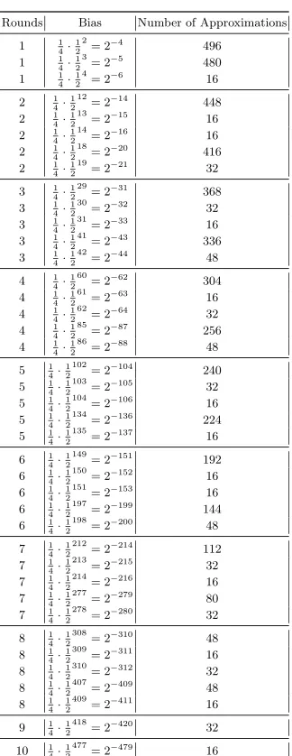
After performing the search in the forward direction, we repeated the experi-ment, this time running the light mask in the backward direction (i.e., throughT−1) as many rounds as possible. The results obtained in these experiments are shown in Tables 1 and 2, which present the number of possible linear approximations of that form in the forward and the backward directions (along with the associated bias). The longest of which covers 10 rounds in any direction.
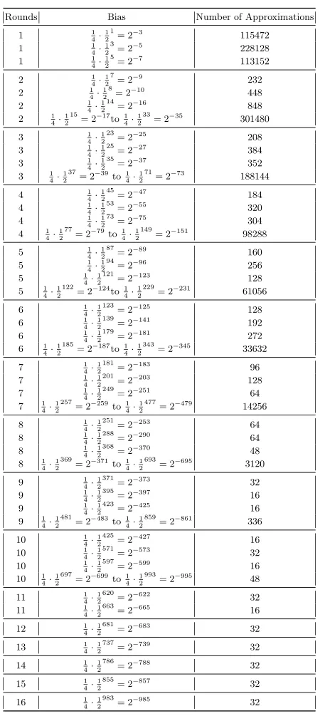
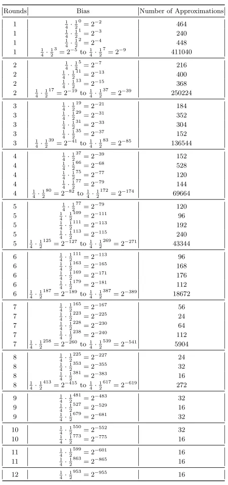
Following the surprisingly long approximations, we decided to explore pairs of pairs (i.e., four active bits in the starting mask), repeating the process of analyzing the forward direction as well as the backward direction. These results are summa-rized in Tables 3 and 4.
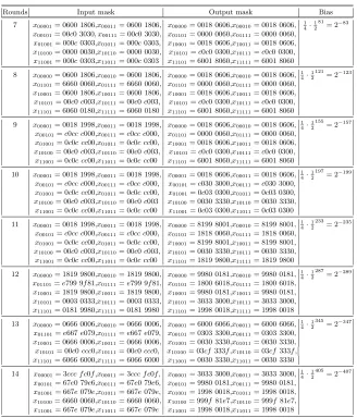
We also combined the forward and the backward approximations to form a series of approximations for as many rounds as could, using the combination of this type of approximations. In Table 5 we offer input/output masks of the best approximations we found.
Following the fact that CubeHash aims to offer at most a 2512
Table 1.Number of Linear Approximations Following the Consecutive Masks Approach (Starting from a Mask with One Consecutive Pair in the Forward Direction)
Rounds Bias Number of Approximations
1 1 4·
1 2 0
= 2−2 480 1 1
4· 1 2 1
= 2−3
16 1 1 4· 1 2 2
= 2−4 480 1 1
4· 1 2 3
= 2−5 16
2 1 4·
1 2 11
= 2−13
432 2 1 4· 1 2 12
= 2−14 16 2 1
4· 1 2 15
= 2−17 16 2 1
4· 1 2 16
= 2−18
416 2 1 4· 1 2 17
= 2−19
16 2 1 4· 1 2 20
= 2−22 16
3 1 4·
1 2 29
= 2−31
384 3 1 4· 1 2 30
= 2−32 16 3 1
4· 1 2 33
= 2−35 16 3 1
4· 1 2 35
= 2−37
352 3 1 4· 1 2 36
= 2−38 16 3 1
4· 1 2 39
= 2−41 16
4 1 4·
1 2 66
= 2−68 336 4 1
4· 1 2 67
= 2−69 16 4 1
4· 1 2 70
= 2−72 16 4 1
4· 1 2 74
= 2−76
288 4 1 4· 1 2 75
= 2−77 16 4 1
4· 1 2 78
= 2−80 16
5 1 4·
1 2
113
= 2−115 272 5 1
4· 1 2
114
= 2−116 240 5 1
4· 1 2
115
= 2−117 16 5 1
4· 1 2
117 = 2−119
16 5 1 4· 1 2 118
= 2−120 16
6 1 4·
1 2
169 = 2−171
208 6 1 4· 1 2 170 = 2−172
16 6 1 4· 1 2 171
= 2−173 160 6 1
4· 1 2
172
= 2−174 16 6 1
4· 1 2
173 = 2−175
16 6 1 4· 1 2 175
= 2−177 16
7 1 4·
1 2
236 = 2−238
96 7 1 4· 1 2 237 = 2−239
16 7 1 4· 1 2 238
= 2−240 144 7 1
4· 1 2
239
= 2−241 16 7 1
4· 1 2
240 = 2−242
16 7 1 4· 1 2 242
= 2−244 16
8 1 4·
1 2
346 = 2−348
32 8 1 4· 1 2 347 = 2−349
16 8 1 4· 1 2 350
= 2−352 16 8 1
4· 1 2
353
= 2−355 80 8 1
4· 1 2
354 = 2−356
16 8 1 4· 1 2 357
= 2−359 16
9 1 4·
1 2
445 = 2−447
16 9 1 4· 1 2 481
= 2−483 32 9 1
4· 1 2
485
= 2−487 16
10 1 4·
1 2
550 = 2−552
16
biases requires more than 2512
Table 2.Number of Linear Approximations Following the Consecutive Masks Approach (Starting from a Mask with One Consecutive Pair in the Backward Direction)
Rounds Bias Number of Approximations
1 1 4·
1 2 2
= 2−4 496 1 1
4· 1 2 3
= 2−5
480 1 1 4· 1 2 4
= 2−6 16
2 1 4·
1 2 12
= 2−14
448 2 1 4· 1 2 13
= 2−15
16 2 1 4· 1 2 14
= 2−16 16 2 1
4· 1 2 18
= 2−20 416 2 1
4· 1 2 19
= 2−21
32 3 1 4· 1 2 29
= 2−31 368 3 1
4· 1 2 30
= 2−32
32 3 1 4· 1 2 31
= 2−33
16 3 1 4· 1 2 41
= 2−43 336 3 1
4· 1 2 42
= 2−44 48
4 1 4·
1 2 60
= 2−62 304 4 1
4· 1 2 61
= 2−63 16 4 1
4· 1 2 62
= 2−64
32 4 1 4· 1 2 85
= 2−87
256 4 1 4· 1 2 86
= 2−88 48
5 1 4·
1 2
102 = 2−104
240 5 1 4· 1 2 103
= 2−105 32 5 1
4· 1 2
104
= 2−106 16 5 1
4· 1 2
134
= 2−136 224 5 1
4· 1 2
135 = 2−137
16 6 1 4· 1 2 149
= 2−151 192 6 1
4· 1 2
150 = 2−152
16 6 1 4· 1 2 151
= 2−153 16 6 1
4· 1 2
197
= 2−199 144 6 1
4· 1 2
198
= 2−200 48
7 1 4·
1 2
212
= 2−214 112 7 1
4· 1 2
213
= 2−215 32 7 1
4· 1 2
214 = 2−216
16 7 1 4· 1 2 277
= 2−279 80 7 1
4· 1 2
278
= 2−280 32
8 1 4·
1 2
308
= 2−310 48 8 1
4· 1 2
309
= 2−311 16 8 1
4· 1 2
310
= 2−312 32 8 1
4· 1 2
407 = 2−409
48 8 1 4· 1 2 409
= 2−411 16
9 1 4·
1 2
418 = 2−420
32 10 1 4· 1 2 477
= 2−479 16
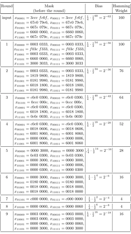
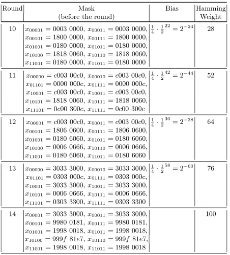
For those interested in assessing the full security that might be offered by the 1024-bit transformationT, we note that there also exists a 14-round linear approxi-mation with a bias of 2−406. We outline the full 14-round approximation in Tables 7 and 8.
4
Message Modification Techniques — A Chosen-Plaintext
Linear Approximations
Math-Table 3.Number of Approximations with a Given Bias Starting from a Pair of Pair of Active Bits (Forward Direction)
Rounds Bias Number of Approximations
1 1
4· 1 2 1
= 2−3 115472
1 1
4· 1 2 3
= 2−5
228128 1 1 4· 1 2 5
= 2−7 113152
2 1
4· 1 2 7
= 2−9
232 2 1 4· 1 2 8
= 2−10
448 2 1 4· 1 2 14
= 2−16 848 2 1
4· 1 2 15
= 2−17to1 4·
1 2 33
= 2−35 301480
3 1
4· 1 2 23
= 2−25 208
3 1
4· 1 2 25
= 2−27 384
3 1
4· 1 2 35
= 2−37
352 3 1 4· 1 2 37
= 2−39to1 4·
1 2 71
= 2−73 188144
4 1
4· 1 2 45
= 2−47 184
4 1
4· 1 2 53
= 2−55 320
4 1
4· 1 2 73
= 2−75 304 4 1
4· 1 2 77
= 2−79to1 4·
1 2
149
= 2−151 98288
5 1
4· 1 2 87
= 2−89 160
5 1
4· 1 2 94
= 2−96 256
5 1
4· 1 2
121
= 2−123 128 5 1
4· 1 2
122 = 2−124
to1 4·
1 2
229 = 2−231
61056 6 1 4· 1 2 123
= 2−125 128
6 1
4· 1 2
139 = 2−141
192 6 1 4· 1 2 179
= 2−181 272 6 1
4· 1 2
185
= 2−187to1 4·
1 2
343
= 2−345 33632
7 1
4· 1 2
181
= 2−183 96
7 1
4· 1 2
201
= 2−203 128
7 1
4· 1 2
249
= 2−251 64 7 1
4· 1 2
257 = 2−259
to1 4·
1 2
477 = 2−479
14256 8 1 4· 1 2 251
= 2−253 64
8 1
4· 1 2
288 = 2−290
64 8 1 4· 1 2 368
= 2−370 48 8 1
4· 1 2
369
= 2−371to1 4·
1 2
693
= 2−695 3120
9 1
4· 1 2
371 = 2−373
32 9 1 4· 1 2 395
= 2−397 16
9 1
4· 1 2
423
= 2−425 16 9 1
4· 1 2
481 = 2−483
to1 4·
1 2
859 = 2−861
336 10 1 4· 1 2 425
= 2−427 16
10 1
4· 1 2
571 = 2−573
32 10 1 4· 1 2 597 = 2−599
16 10 1 4· 1 2 697
= 2−699to1 4·
1 2
993
= 2−995 48
11 1
4· 1 2
620 = 2−622
32 11 1 4· 1 2 663
= 2−665 16
12 1
4· 1 2
681 = 2−683
32 13 1 4· 1 2 737
= 2−739 32
14 1
4· 1 2
786
= 2−788 32
15 1
4· 1 2
855 = 2−857
32 16 1 4· 1 2 983
= 2−985 32
Table 4.Number of Approximations with a Given Bias Starting from a Pair of Pair of Active Bits (Backward Direction)
Rounds Bias Number of Approximations
1 1
4· 1 2 0
= 2−2 464
1 1
4· 1 2 1
= 2−3
240 1 1 4· 1 2 2
= 2−4 448
1 1
4· 1 2 3
= 2−5to1 4·
1 2 7
= 2−9 411040
2 1
4· 1 2 5
= 2−7 216
2 1
4· 1 2 11
= 2−13 400
2 1
4· 1 2 13
= 2−15 368 2 1
4· 1 2 17
= 2−19 to1
4· 1 2 37
= 2−39
250224 3 1 4· 1 2 19
= 2−21 184
3 1
4· 1 2 29
= 2−31
352 3 1 4· 1 2 31
= 2−33 304
3 1
4· 1 2 35
= 2−37 152 3 1
4· 1 2 39
= 2−41to1 4·
1 2 83
= 2−85 136544
4 1
4· 1 2 37
= 2−39 152
4 1
4· 1 2 66
= 2−68 528
4 1
4· 1 2 75
= 2−77
120 4 1 4· 1 2 77
= 2−79 144 4 1
4· 1 2 80
= 2−82to1 4·
1 2
172
= 2−174 69664
5 1
4· 1 2 77
= 2−79
120 5 1 4· 1 2 109
= 2−111 96
5 1
4· 1 2
111
= 2−113 192
5 1
4· 1 2
113 = 2−115
240 5 1 4· 1 2 125
= 2−127to1 4·
1 2
269
= 2−271 43344
6 1
4· 1 2
111 = 2−113
96 6 1 4· 1 2 163 = 2−165
168 6 1 4· 1 2 169
= 2−171 176
6 1
4· 1 2
179
= 2−181 112 6 1
4· 1 2
187 = 2−189
to1 4·
1 2
387 = 2−389
18672 7 1 4· 1 2 165
= 2−167 56
7 1
4· 1 2
223
= 2−225 24
7 1
4· 1 2
228
= 2−230 64
7 1
4· 1 2
238
= 2−240 112 7 1
4· 1 2
258
= 2−260to1 4·
1 2
539
= 2−541 5904
8 1
4· 1 2
225
= 2−227 24
8 1
4· 1 2
353
= 2−355 32
8 1
4· 1 2
381
= 2−383 16 8 1
4· 1 2
413
= 2−415to1 4·
1 2
617
= 2−619 272
9 1
4· 1 2
481
= 2−483 32
9 1
4· 1 2
527 = 2−529
16 9 1 4· 1 2 679
= 2−681 32
10 1
4· 1 2
550 = 2−552
32 10 1 4· 1 2 773
= 2−775 16
11 1
4· 1 2
599 = 2−601
16 11 1 4· 1 2 863
= 2−865 16
12 1
4· 1 2
953
= 2−955 16
In the case of modular addition, the linear approximation which we use is satis-fied whenever one of the LSBs of the approximated bits is 0. This allows preselecting inputs for which the approximation holds with probability 1.
Table 5.A trade-off of biases and rounds. Each line shows the best bias in this setting
Rounds Input mask Output mask Bias
7 x00001= 0600 1806,x00011= 0600 1806, x00000= 0018 0606,x00010= 0018 0606, 14· 1 2 81
= 2−83
x00101= 00c0 3030, x00111= 00c0 3030, x01101= 0000 0060,x01111= 0000 0060,
x01001= 000c0303,x01011= 000c0303, x10001= 0018 0606,x10011= 0018 0606,
x10100= 0000 0030,x10110= 0000 0030, x10101=c0c0 0300,x10111=c0c0 0300,
x11001= 000c0303,x11011= 000c0303 x11101= 6001 8060,x11111= 6001 8060
8 x00000= 0600 1806,x00010= 0600 1806, x00000= 0018 0606,x00010= 0018 0606, 1 4·
1 2
121 = 2−123
x01101= 6660 0060,x01111= 6660 0060, x01101= 0000 0060,x01111= 0000 0060,
x10001= 0600 1806,x10011= 0600 1806, x10001= 0018 0606,x10011= 0018 0606,
x10101= 00c0c003,x10111= 00c0c003, x10101=c0c0 0300,x10111=c0c0 0300,
x11101= 6060 0180,x11111= 6060 0180 x11101= 6001 8060,x11111= 6001 8060
9 x00001= 0018 1998,x00011= 0018 1998, x00000= 0018 0606,x00010= 0018 0606, 14·12 155
= 2−157
x00101=c0cc c000,x00111=c0cc c000, x01101= 0000 0060,x01111= 0000 0060,
x01001= 0c0c cc00,x01011= 0c0c cc00, x10001= 0018 0606,x10011= 0018 0606,
x10100= 00c0c003,x10110= 00c0c003, x10101=c0c0 0300,x10111=c0c0 0300,
x11001= 0c0c cc00,x11011= 0c0c cc00 x11101= 6001 8060,x11111= 6001 8060
10 x00001= 0018 1998,x00011= 0018 1998, x00001= 0018 0606,x00011= 0018 0606, 14· 1 2
197 = 2−199
x00101=c0cc c000,x00111=c0cc c000, x00101=c030 3000,x00111=c030 3000,
x01001= 0c0c cc00,x01011= 0c0c cc00, x01001= 0c03 0300,x01011= 0c03 0300,
x10100= 00c0c003,x10110= 00c0c003 x10100= 0030 3330,x10110= 0030 3330,
x11001= 0c0c cc00,x11011= 0c0c cc00 x11001= 0c03 0300,x11011= 0c03 0300
11 x00001= 0018 1998,x00011= 0018 1998, x00000= 8199 8001,x00010= 8199 8001, 1 4·
1 2
233 = 2−235
x00101=c0cc c000,x00111=c0cc c000, x01101= 1818 0060,x01111= 1818 0060,
x01001= 0c0c cc00,x01011= 0c0c cc00, x10001= 8199 8001,x10011= 8199 8001,
x10100= 00c0c003,x10110= 00c0c003, x10101= 0030 3330,x10111= 0030 3330,
x11001= 0c0c cc00,x11011= 0c0c cc00 x11101= 1819 9800,x11111= 1819 9800
12 x00000= 1819 9800,x00010= 1819 9800, x00000= 9980 0181,x00010= 9980 0181, 14·12 287
= 2−289
x01101=e799 9f81,x01111=e799 9f81, x01101= 1800 6018,x01111= 1800 6018,
x10001= 1819 9800,x10011= 1819 9800, x10001= 9980 0181,x10011= 9980 0181,
x10101= 0003 0333,x10111= 0003 0333, x10101= 3033 3000,x10111= 3033 3000,
x11101= 0181 9980,x11111= 0181 9980 x11101= 1998 0018,x11111= 1998 0018
13 x00000= 0666 0006,x00010= 0666 0006, x00001= 6000 6066,x00011= 6000 6066, 14· 1 2
345 = 2−347
x01101=e667e079,x01111=e667e079, x00101= 0303 3300,x00111= 0303 3300,
x10001= 0666 0006,x10011= 0666 0006, x01001= 0030 3330,x01011= 0030 3330,
x10101= 00c0ccc0,x10111= 00c0ccc0, x10100= 03cf333f,x10110= 03cf333f,
x11101= 6066 6000,x11111= 6066 6000 x11001= 0030 3330,x11011= 0030 3330
14 x00001= 3ccc f c0f,x00011= 3ccc f c0f, x00001= 3033 3000,x00011= 3033 3000, 1 4·
1 2
405 = 2−407
x00101= 67e0 79e6,x00111= 67e0 79e6, x00101= 9980 0181,x00111= 9980 0181,
x01001= 667e079e,x01011= 667e079e, x01001= 1998 0018,x01011= 1998 0018,
x10100= 6660 0060,x10110= 6660 0060, x10100= 999f81e7,x10110= 999f81e7,
x11001= 667e079e,x11011= 667e079e x11001= 1998 0018,x11011= 1998 0018
0008 0888x, x10101= 1100 0101x, x10111 = 1100 0101x and the whole wordsx11101
andx11111. We note that one can pick other sets of bits (where any fixed bit from
x0jklm can be exchanged for a bit inx1jklm).
Fixing bits for the next layer is a bit more tricky, as it requires to fix some internal state bit (after an XOR or addition) is 0. This task is a bit harder due to carry issues. More precisely, to fix bit iof x1jklm after the first five operations of
T, it is required that bitiofx1jklmis 0 after the first operation ofT. This specific bit depends on the corresponding carry chain.
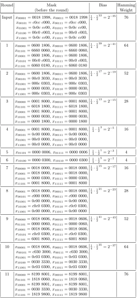
Table 6.The 11-round linear approximation with bias 1 4 ·
1 2
233
= 2−235
Round Mask Bias Hamming
(before the round) Weight
Input x00001= 0018 1998,x00011= 0018 1998 1 4·
1 2 33
= 2−35 76
x00101=c0cc c000,x00111=c0cc c000,
x01001= 0c0c cc00,x01011= 0c0c cc00,
x10100= 00c0c003,x10110= 00c0c003,
x11001= 0c0c cc00,x11011= 0c0c cc00
1 x00000= 0600 1806,x00010= 0600 1806,14·12 39
= 2−41 64
x01101= 6660 0060,x01111= 6660 0060,
x10001= 0600 1806,x10011= 0600 1806,
x10101= 00c0c003,x10111= 00c0c003,
x11101= 6060 0180,x11111= 6060 0180
2 x00001= 0600 1806,x00011= 0600 1806,14· 1 2 17
= 2−19 52
x00101= 00c0 3030,x00111= 00c0 3030,
x01001= 000c0303,x01011= 000c0303,
x10100= 0000 0030,x10110= 0000 0030,
x11001= 000c0303,x11011= 000c0303
3 x00000= 0001 8000,x00010= 0001 8000,14· 1 2 13
= 2−15 28
x01101= 6018 1800,x01111= 6018 1800,
x10001= 0001 8000,x10011= 0001 8000,
x10101= 0000 0030,x10111= 0000 0030,
x11101= 0000 1800,x11111= 0000 1800
4 x00001= 0001 8000,x00011= 0001 8000, 14·12 3
= 2−5 16
x00101= 0c00 0000,x00111= 0c00 0000,
x01001= 00c0 0000,x01011= 00c0 0000,
x11001= 00c0 0000,x11011= 00c0 0000
5 x01101= 0000 0006,x01111= 0000 0006 14· 1 2 1
= 2−3 4
6 x10100= 0000 0300,x10110= 0000 0300 14· 1 2 5
= 2−7 4
7 x00000= 0018 0000,x00010= 0018 0000,14·12 15
= 2−17 16
x10001= 0018 0000,x10011= 0018 0000,
x10101= 0000 0300,x10111= 0000 0300,
x11101= 0001 8000,x11111= 0001 8000
8 x00001= 0018 0000,x00011= 0018 0000,14· 1 2 21
= 2−23 28
x00101=c000 0000,x00111=c000 0000,
x01001= 0c00 0000,x01011= 0c00 0000,
x10100=c0c0 0300,x10110=c0c0 0300,
x11001= 0c00 0000,x11011= 0c00 0000
9 x00000= 0018 0606,x00010= 0018 0606,14·12 41
= 2−43 52
x01101= 0000 0060,x01111= 0000 0060,
x10001= 0018 0606,x10011= 0018 0606,
x10101=c0c0 0300,x10111=c0c0 0300,
x11101= 6001 8060,x11111= 6001 8060
10 x00001= 0018 0606,x00011= 0018 0606,14· 1 2 35
= 2−37 64
x00101=c030 3000,x00111=c030 3000,
x01001= 0c03 0300,x01011= 0c03 0300,
x10100= 0030 3330,x10110= 0030 3330,
x11001= 0c03 0300,x11011= 0c03 0300
11 x00000= 8199 8001,x00010= 8199 8001, 76
x01101= 1818 0060,x01111= 1818 0060,
x10001= 8199 8001,x10011= 8199 8001,
x10101= 0030 3330,x10111= 0030 3330,
x11101= 1819 9800,x11111= 1819 9800
As the above approach sets many bits to zero (namely 33 bits to increase the bias by a factor 2), we offer a more efficient approach. One can fix only bitsi−1, iin
Table 7.The 14-round linear approximation with bias 1 4 ·
1 2
405
= 2−407 rounds 1-9
Round Mask Bias Hamming
(before the round) Weight
input x00001= 3ccc f c0f,x00011= 3ccc f c0f, 1 4·
1 2 60
= 2−62 160
x00101= 67e0 79e6,x00111= 67e0 79e6,
x01001= 667e079e,x01011= 667e079e,
x10100= 6660 0060,x10110= 6660 0060,
x11001= 667e079e,x11011= 667e079e
1 x00000= 0003 0333,x00010= 0003 0333, 14·12 54
= 2−56 100
x01101=f03c f333,x01111=f03c f333,
x10001= 0003 0333,x10011= 0003 0333,
x10101= 6660 0060,x10111= 6660 0060,
x11101= 3000 3033,x11111= 3000 3033
2 x00001= 0003 0333,x00011= 0003 0333, 14· 1 2 34
= 2−36 76
x00101= 1819 9800,x00111= 1819 9800,
x01001= 0181 9980,x01011= 0181 9980,
x10100= 6018 1800,x10110= 6018 1800,
x11001= 0181 9980,x11011= 0181 9980
3 x00000=c0c0 0300,x00010=c0c0 0300, 1 4·
1 2 40
= 2−42 64
x01101= 0ccc000c,x01111= 0ccc000c,
x10001=c0c0 0300,x10011=c0c0 0300,
x10101= 6018 1800,x10111= 6018 1800,
x11101= 0c0c0030,x11111= 0c0c0030
4 x00001=c0c0 0300,x00011=c0c0 0300, 14·12 18
= 2−20 52
x00101= 0018 0606,x00111= 0018 0606,
x01001= 6001 8060,x01011= 6001 8060,
x10100= 0000 0006,x10110= 0000 0006,
x11001= 6001 8060,x11011= 6001 8060
5 x00000= 0000 3000,x00010= 0000 3000 ,14· 1 2 14
= 2−16 28
x01101= 0c03 0300,x01111= 0c03 0300,
x10001= 0000 3000,x10011= 0000 3000,
x10101= 0000 0006,x10111= 0000 0006,
x11101= 0000 0300,x11111= 0000 0300
6 x00001= 0000 3000,x00011= 0000 3000, 1 4·
1 2 4
= 2−6 16
x00101= 0180 0000,x00111= 0180 0000,
x01001= 0018 0000,x01011= 0018 0000,
x11001= 0018 0000,x11011= 0018 0000
7 x01101=c000 0000,x01111=c000 0000 14· 1 2 2
= 2−4 4
8 x10100= 0000 0060,x10110= 0000 0060 14·12 6
= 2−8 4
9 x00000= 0003 0000,x00010= 0003 0000, 1 4·
1 2 16
= 2−18 16
x10001= 0003 0000,x10011= 0003 0000,
x10101= 0000 0060,x10111= 0000 0060,
x11101= 0000 3000,x11111= 0000 3000
zero one needs to set the mask bits masked by 000c 0cccx ofx00001, x00011, x10001,
andx10011, the bits masked byc00c0001xofx00101, x00111, x10101, and x10111, and
those masked by 0c0c cc00 inx01000, x01001, x01010, x01011, x11000, x11001, x11010, and x11011 to zero. Fixing these 116 bits (10 of which are shared with the previous 80),
assures that all the additions in the first round of the 12-round approximation follow the approximation, i.e., “saving” their “contribution” to the bias, and resulting in a bias of 1
4· 1 2
233
= 2−235.
We note that the number of bits set to 0 is 186, leaving 838 bits to be randomly selected. This is sufficient to generate the 2470
possible inputs to T12
Table 8.The 14-round linear approximation with bias 1 4 ·
1 2
405
= 2−407 rounds 10-14
Round Mask Bias Hamming
(before the round) Weight
10 x00001= 0003 0000,x00011= 0003 0000, 1 4·
1 2 22
= 2−24 28
x00101= 1800 0000,x00111= 1800 0000,
x01001= 0180 0000,x01011= 0180 0000,
x10100= 1818 0060,x10110= 1818 0060,
x11001= 0180 0000,x11011= 0180 0000
11 x00000=c003 00c0,x00010=c003 00c0, 14·12 42
= 2−44 52
x01101= 0000 000c,x01111= 0000 000c,
x10001=c003 00c0,x10011=c003 00c0,
x10101= 1818 0060,x10111= 1818 0060,
x11101= 0c00 300c,x11111= 0c00 300c
12 x00001=c003 00c0,x00011=c003 00c0, 14· 1 2 36
= 2−38 64
x00101= 1806 0600,x00111= 1806 0600,
x01001= 0180 6060,x01011= 0180 6060,
x10100= 0006 0666,x10110= 0006 0666,
x11001= 0180 6060,x11011= 0180 6060
13 x00000= 3033 3000,x00010= 3033 3000, 1 4·
1 2 58
= 2−60 76
x01101= 0303 000c,x01111= 0303 000c,
x10001= 3033 3000,x10011= 3033 3000,
x10101= 0006 0666,x10111= 0006 0666,
x11101= 0303 3300,x11111= 0303 3300
14 x00001= 3033 3000,x00011= 3033 3000, 100
x00101= 9980 0181,x00111= 9980 0181,
x01001= 1998 0018,x01011= 1998 0018,
x10100= 999f81e7,x10110= 999f81e7,
x11001= 1998 0018,x11011= 1998 0018
Table 9.The round that extends the 11-round approximation to 12 rounds (and the bits to fix
Round Input mask Input bits fixed to 0 -1 x00000= 0018 1998,x00010= 0018 1998 x10001= 0008 0888x,x10011= 0008 0888x
x01101= 81e7 999f,x01111= 81e7 999f x10101= 1100 0101x,x10111= 1100 0101x x10001= 0018 1998,x10011= 0018 1998 x11101=f f f f f f f fx,x11111=f f f f f f f fx x10101= 3300 0303,x10111= 3300 0303
x11101= 8001 8199,x11111= 8001 8199
-0.5 x00101=f30c0300x,x00111=f30c0300x x00001= 000c0cccx,x00011= 000c0cccx x01000= 0c0c cc00x,x01001= 0c0c cc00x x00101=c00c0001x,x00111=c00c0001x x01010= 0c0c cc00x,x01011= 0c0c cc00x x01000= 0c0c cc00x,x01001= 0c0c cc00x x01101= 8001 8199x,x01111= 8001 8199x x01010= 0c0c cc00x,x01011= 0c0c cc00x x10001= 0018 1998x,x10011= 0018 1998x x10001= 000c0cccx,x10011= 000c0cccx x10101=c00c003,x10111=c00c003 x10101=c00c0001x,x10111=c00c0001x x11000= 0c0c cc00x,x11001= 0c0c cc00x x11010= 0c0c cc00x,x11011= 0c0c cc00x x11010= 0c0c cc00x,x11011= 0c0c cc00x x10001= 000c0cccx,x10011= 000c0cccx
0 x00001= 0018 1998,x00011= 0018 1998
x00101=c0cc c000,x00111=c0cc c000
x01001= 0c0c cc00,x01011= 0c0c cc00
x10100= 00c0c003,x10110= 00c0c003
x11001= 0c0c cc00,x11011= 0c0c cc00
−0.5 stands for the mask that enters the second addition of the additional round.
5
Distinguishing Reduced-Round Variants of the
Compression Function of CubeHash
by just comparing the input/output of a few queries to the black box with the input/output produced by the publicly available algorithm. If we want to offer some cryptographic settings in which distinguishing attacks make sense, we either need to consider keyed variants (either of the round functionT or of the hash function, e.g., in MACs) or to discuss known-key distinguishers [23].
Such possible “application” is an a Even-Mansour [15] variant of 11-roundT (or any other number of rounds), i.e., EM-T11
k1,k2(P) = T
11
(P⊕k1)⊕k2. If 11-round T is indeed good as a source of nonlinearity (for a linear T, the entire security of CubeHash collapses), then XORing an unknown key before and after these 11 rounds, should result in a good pseudo-random permutation. Using our linear ap-proximations, one can distinguish this construction from a random permutation.
We emphasize that as our results are linear in nature, they require that the adversary has access both to the input to the nonlinear function as well as its output. To the best of our knowledge, there is no way to use this directly in a hash function setting.
6
Conclusions
In this paper we presented a series of approximations for the SHA-3 candidate CubeHash. The analysis challenges the strength of CubeHash’s round function,T, and shows that (from linear cryptanalysis point of view), offers adequate security. At the same time, the security margins offered by 16 iterations ofT seems to be on the smaller side, as future works on CubeHash may find better linear approximations.
Acknowledgement
The authors wish to thank Prof. Adi Shamir for his guidance and assistance an-alyzing CubeHash, Nathan Keller for providing core ideas in this paper, Daniel J. Bernstein for his insightful and mind-provoking comments on previous versions of this article. Finally, we wish to thank Michael Klots for his technical assistance, which was crucial for finding our results.
References
1. Andreeva, E., Bouillaguet, C., Fouque, P.A., Hoch, J.J., Kelsey, J., Shamir, A., Zim-mer, S.: Second Preimage Attacks on Dithered Hash Functions. In Smart, N.P., ed.: EUROCRYPT. Volume 4965 of Lecture Notes in Computer Science., Springer (2008) 270–288
2. Aumasson, J.P.: Collision for CubeHash2/120-512. NIST mailing list (2008) Available online at http://ehash.iaik.tugraz.at/uploads/a/a9/Cubehash.txt.
3. Aumasson, J.P., Brier, E., Meier, W., Naya-Plasencia, M., Peyrin, T.: Inside the Hypercube. In Boyd, C., Nieto, J.M.G., eds.: ACISP. Volume 5594 of Lecture Notes in Computer Science., Springer (2009) 202–213
4. Bernstein, D.J.: CubeHash specification (2.B.1). Submission to NIST (2008) 5. Bernstein, D.J.: CubeHash specification (2.B.1). Submission to NIST (2009) 6. Biham, E., Chen, R.: Near-Collisions of SHA-0. [17] 290–305
7. Bloom, B., Kaminsky, A.: Single Block Attacks and Statistical Tests on CubeHash. IACR ePrint Archive, Report 2009/407 (2009)
9. Brier, E., Khazaei, S., Meier, W., Peyrin, T.: Real Collisions
for CubeHash-4/48. NIST mailing list (2009) Available online at
http://ehash.iaik.tugraz.at/uploads/5/50/Bkmp ch448.txt.
10. Brier, E., Khazaei, S., Meier, W., Peyrin, T.: Real Collisions
for CubeHash-4/64. NIST mailing list (2009) Available online at
http://ehash.iaik.tugraz.at/uploads/9/93/Bkmp ch464.txt.
11. Canni`ere, C.D., Rechberger, C.: Finding SHA-1 Characteristics: General Results and Applications. In Lai, X., Chen, K., eds.: ASIACRYPT. Volume 4284 of Lecture Notes in Computer Science., Springer (2006) 1–20
12. Cho, J.Y., Pieprzyk, J.: Multiple Modular Additions and Crossword Puzzle Attack on NLSv2. In Garay, J.A., Lenstra, A.K., Mambo, M., Peralta, R., eds.: ISC. Volume 4779 of Lecture Notes in Computer Science., Springer (2007) 230–248
13. Cramer, R., ed.: Advances in Cryptology - EUROCRYPT 2005, 24th Annual Inter-national Conference on the Theory and Applications of Cryptographic Techniques, Aarhus, Denmark, May 22-26, 2005, Proceedings. In Cramer, R., ed.: EUROCRYPT. Volume 3494 of Lecture Notes in Computer Science., Springer (2005)
14. Dai, W.: Collisions for CubeHash1/45 and CubeHash2/89 (2008) Available online at http://www.cryptopp.com/sha3/cubehash.pdf.
15. Even, S., Mansour, Y.: A Construction of a Cipher from a Single Pseudorandom Permutation. J. Cryptology 10(3) (1997) 151–162
16. Ferguson, N., Lucks, S., McKay, K.A.: Symmetric States and their Structure: Improved Analysis of CubeHash. IACR ePrint Archive, Report 2010/273 (2010) Presented at the SHA-3 second workshop, Santa Barbara, USA, August 23-24, 2010.
17. Franklin, M.K., ed.: Advances in Cryptology - CRYPTO 2004, 24th Annual Inter-national CryptologyConference, Santa Barbara, California, USA, August 15-19, 2004, Proceedings. In Franklin, M.K., ed.: CRYPTO. Volume 3152 of Lecture Notes in Computer Science., Springer (2004)
18. Joux, A.: Multicollisions in Iterated Hash Functions. Application to Cascaded Con-structions. [17] 306–316
19. Kelsey, J., Kohno, T.: Herding Hash Functions and the Nostradamus Attack. In Vaudenay, S., ed.: EUROCRYPT. Volume 4004 of Lecture Notes in Computer Science., Springer (2006) 183–200
20. Kelsey, J., Schneier, B.: Second Preimages on n-Bit Hash Functions for Much Less than 2n Work. [13] 474–490
21. Khovratovich, D., Nikolic’, I., Weinmann, R.P.: Preimage attack on
CubeHash512-r/4 and CubeHash512-r/8 (2008) Available online at
http://ehash.iaik.tugraz.at/uploads/6/6c/Cubehash.pdf.
22. Knudsen, L.R., Mathiassen, J.E.: A Chosen-Plaintext Linear Attack on DES. In Schneier, B., ed.: FSE. Volume 1978 of Lecture Notes in Computer Science., Springer (2000) 262–272
23. Knudsen, L.R., Rijmen, V.: Known-Key Distinguishers for Some Block Ciphers. In Kurosawa, K., ed.: ASIACRYPT. Volume 4833 of Lecture Notes in Computer Science., Springer (2007) 315–324
24. Matsui, M.: Linear Cryptoanalysis Method for DES Cipher. In: EUROCRYPT. (1993) 386–397
25. National Institute of Standards and Technology: Cryptographic Hash Algorithm Com-petition. http://www.nist.gov/hash-competition (2008)
26. Stevens, M., Lenstra, A.K., de Weger, B.: Chosen-Prefix Collisions for MD5 and Colliding X.509 Certificates for Different Identities. In Naor, M., ed.: EUROCRYPT. Volume 4515 of Lecture Notes in Computer Science., Springer (2007) 1–22