Autonomous and Real Time Rock Image Classification using Convolutional Neural Networks

(1)

Scholarship@Western

Electronic Thesis and Dissertation Repository

2-8-2019 11:00 AM

Autonomous and Real Time Rock Image Classification using

Convolutional Neural Networks

Alexis David Pascual

The University of Western Ontario Supervisor

McIsaac, Ken

The University of Western Ontario Co-Supervisor Osinski, Gordon

The University of Western Ontario

Graduate Program in Electrical and Computer Engineering

A thesis submitted in partial fulfillment of the requirements for the degree in Master of Engineering Science

Follow this and additional works at: https://ir.lib.uwo.ca/etd Part of the Electrical and Computer Engineering Commons

Recommended Citation Recommended Citation

Pascual, Alexis David, "Autonomous and Real Time Rock Image Classification using Convolutional Neural Networks" (2019). Electronic Thesis and Dissertation Repository. 6059.

https://ir.lib.uwo.ca/etd/6059

This Dissertation/Thesis is brought to you for free and open access by Scholarship@Western. It has been accepted for inclusion in Electronic Thesis and Dissertation Repository by an authorized administrator of

(2)

classification algorithm to classify 9 different types of rock images using a with the image fea-tures extracted autonomously. Through this method, they achieved a test accuracy of 96.71%.

Within the last few years, Convolutional Neural Networks (CNNs) have been shown to be

per-form better than other algorithms in classifying images of everyday objects. In light of this

development, this thesis demonstrates the use of CNNs to classify the same set of rock images.

With the addition of dataset augmentation, a 3-layer CNN is shown to have a significant

im-provement over Shu et. al.’s results, achieving an average accuracy of 99.60% across 10 trials

on the test set. Multiple CNN operations with similar output shapes have been designed and

appended to an existing architecture to expand hyperparameter considerations. These

Com-binational Fully Connected Neural Networks achieves an accuracy of 99.36% on the test set.

The resulting models are also shown to be lightweight enough that they can be deployed on

a mobile device. To tackle a more interesting and practical problem, CNNs have also been

designed to classify natural scene images of rocks, an inherently more complex dataset. The

task has been simplified into a binary classification problem where the images are classified

into breccia and non-breccia. This thesis shows that a Combinational Fully Connected Neural

Network achieves an accuracy of 93.50%, better than a 5-layer CNN, which achieves 89.43%.

Keywords: Computer Vision, Machine Learning, Convolutional Neural Networks,

Geol-ogy, Planetary Science, Planetary Exploration

(3)

Abstract i

List of Figures vi

List of Tables ix

List of Appendices x

1 Introduction 1

1.1 Motivation . . . 1

1.2 Tasks and Thesis Contribution . . . 3

1.3 Thesis Outline . . . 3

2 Review of Related Literature 4 2.1 Images and Image Classification . . . 4

2.1.1 An introduction to images . . . 4

2.1.2 Image Feature Representations . . . 7

First-Order Statistics . . . 8

Second-Order Statistics from Gray Level Co-occurence Matrices . . . . 8

2.2 Training a Classifier . . . 11

2.3 Classification Algorithms . . . 12

2.3.1 Unsupervised learning . . . 12

K-means . . . 12

Anomaly Detection . . . 13

2.3.2 Supervised learning . . . 14

Logistic Regression . . . 15

(4)

2.5.1 AlexNet and the Rise of ConvNets . . . 27

2.5.2 Defining Convolutional Neural Networks . . . 29

Convolutional Layer . . . 29

Pooling Layer . . . 32

Fully Connected Layers . . . 33

2.6 ConvNet Architectures . . . 34

AlexNet . . . 34

VGG . . . 35

ResNet . . . 37

Inception, InceptionV2, and InceptionV3 . . . 38

DenseNet . . . 43

MobileNet . . . 44

2.7 Transfer Learning . . . 44

2.8 Implementation . . . 46

3 Rock Image Classification with Convolutional Neural Networks 48 3.1 Related Work . . . 48

Manual Feature Selection . . . 49

Unsupervised Feature Selection . . . 50

Shu et. al.’s Results . . . 51

3.2 Applying a Convolutional Neural Network on the Dataset . . . 51

3.2.1 Data Augmentation . . . 52

3.2.2 Transfer Learning . . . 53

(5)

Transfer Learning Results . . . 55

3.2.3 Training a Custom Network from Scratch . . . 57

Experimental Setup . . . 57

Results . . . 58

Experimental Setup II . . . 60

Results II . . . 60

3.2.4 Fully Connected Combinational Network . . . 62

Results . . . 66

3.3 Model Deployment on an iPad . . . 66

3.4 Summary . . . 68

4 Natural Scene Rock Image Classification 69 4.1 Related Work . . . 70

4.2 ConvNets on Natural Scene Rock Images . . . 72

4.2.1 Dataset . . . 72

4.2.2 Transfer Learning . . . 75

Results . . . 77

4.2.3 Custom Networks . . . 78

Results . . . 79

4.3 Summary . . . 81

5 Conclusion 83 5.1 Summary . . . 83

5.2 Future Work . . . 85

A Training and Validation Graphs for Chapter 3: 9-Class Rock Dataset 86

B Training and Validation Graphs for Chapter 4: Breccia vs Non-Breccia 93

(6)

(7)

2.1 Image Recognition is being able to tell that this is an image of a dog and Object

Detection is pointing out where in the image is the dog. Image courtesy of

Tamu and Dr. Hanif Ladak . . . 5

2.2 Color Map. Image reproduced from [8]. . . 5

2.3 Image broken down to individual RGB channels. . . 6

2.4 Histogram of a sample image. . . 7

2.5 Image example for GLCM creation. Image referenced from [15]. . . 9

2.6 GLCM reference table. (i,j) is the number of times pixel values i and j have been neighbours with each other in one particular direction. . . 9

2.7 GLCM values for a given image in Figure 2.5. . . 10

2.8 K-means algorithm visualization. a) Unclassified data points. b) Initialization of two centroids denoted by the red and blue ”x”. c) The data points are labelled according to their proximity with the centroid. d) The centroids are adjusted to reflect the average of all points belonging to its own class label. The data points are then re-labelled, based on proximity with the new centroids. e,f) The process is repeated until no new data points are re-labelled to a different class. Image taken from [16]. . . 13

2.9 Point anomaly illustration . . . 14

2.10 Sigmoid Function Graph. Image taken from [19]. . . 17

2.11 SVM visualization. . . 17

2.12 KNN Visualization. . . 18

2.13 Decision Tree Visualization taken from [20]. . . 19

2.14 ANN Neuron illustration. . . 19

(8)

2.19 Convolution Demonstration. . . 30

2.20 Edge Detection with Sobel Kernels. Top: horizontal edge detection kernel. Bottom: vertical edge detection kernel . . . 32

2.21 Rectified Linear Units activation function graph. . . 32

2.22 Max Pooling. . . 33

2.23 AlexNet Simplified. . . 34

2.24 AlexNet feature map visualization taken with permission from [43]. . . 36

2.25 VGG Architecture taken with permission from [48]. . . 37

2.26 Residual Networks Building Blocks taken with permission from [50]. . . 38

2.27 34-layer Residual Network Architecture taken with permission from [50]. . . . 39

2.28 Inception Module taken with permission from [52]. . . 41

2.29 GoogleNet architecture taken with permission from [52]. . . 42

2.30 Inception V3 Module taken with permission from [56]. . . 43

2.31 Inception-Resnet Module A taken with permission from [55]. . . 43

2.32 DenseNet Module taken with permission from [57]. . . 44

2.33 MobileNet splitting convolution layer into depth-wise convolution and point-wise convolutions. Image taken from [58]. . . 45

3.1 Sample image for each class in Shu et. al.’s dataset [7]. From top to bottom, left to right: Andesite, Dolostone, Granite, Limestone, Oolitic Limestone, Peri-dotite, Red Granite, Rhyolite, Volcanic Breccia. . . 49

3.2 Unsupervised Feature Learning Diagram. Image taken with permission from [7]. 51 3.3 Data Augmentation Operations. . . 53

(9)

3.6 Screenshots of an iPhone simulator to test the functionality of the app. . . 67

4.1 Sample rock images in Dunlop et. al.’s dataset [73]. . . 70

4.2 Individual rocks segmented from the original image taken from [73]. . . 71

4.3 Results of rock image classification from [73]. . . 72

4.4 Sample images from the database. . . 73

4.5 Sample images in the database of different rocks that contain similarly looking rock hammers. . . 74

4.6 Sample Breccia Image. . . 75

4.7 Sample Non-Breccia Image. . . 76

4.8 Cropped Breccia Images. . . 77

4.9 Cropped Non-Breccia Images. . . 77

4.10 Breccia CFCN Model Architecture. . . 82

A.1 Training and validation graphs for VGG16, VGG19, and ResNet50. . . 87

A.2 Training and validation graphs for MobileNet, InceptionV3, and InceptionRes-NetV2. . . 88

A.3 Training and validation graphs for the DenseNet networks. . . 89

A.4 Training and validation graphs for the 1-layer networks. . . 90

A.5 Training and validation graphs for the 1-layer networks. . . 91

A.6 2 Layer and 3 Layer network loss and accuracy during training. . . 92

A.7 CFCN loss and accuracy during training. . . 92

B.1 Training and validation graphs for VGG16, VGG19, and ResNet50. . . 94

B.2 Training and validation graphs for MobileNet, InceptionV3, and InceptionRes-NetV2. . . 95

B.3 Training and validation graphs for the DenseNet networks. . . 96

B.4 2 Layer and 3 Layer network loss and accuracy during training. . . 97

(10)

3.2 Results from [7]. . . 52

3.3 Pre-trained networks number of trainable parameters. . . 55

3.4 Transfer learning results for each network. . . 56

3.5 Custom Networks number of trainable parameters. . . 58

3.6 Custom Networks number of trainable parameters. . . 58

3.7 Custom Networks Results. . . 59

3.9 Custom Networks Average Accuracy and Loss across 10 trials. . . 61

3.10 Output shape for each layer in the 3-layer network. . . 62

3.11 Output shape for each layer in another 3-layer network that follows the same ”path” as the previously created 3-layer network. . . 63

3.12 Output shape for each layer in another network that follows the same ”path” as the previously created 3-layer network. . . 63

3.13 Combinational Fully Connected Network Results. . . 66

3.14 iPad deployment results. . . 67

4.1 Hyperparameters used for Transfer Learning as well as training the custom networks. . . 78

4.2 Transfer learning results for each network. . . 79

4.3 Custom linear network architecture with 5 convolutional layers. . . 80

(11)

Appendix A Training and Validation Graphs for Chapter 3: 9-Class Rock Dataset . . . . 86

Appendix B Training and Validation Graphs for Chapter 4: Breccia vs Non-Breccia . . . 93

(12)

1.1 Motivation

Traditionally, geological exploration and mapping is a tedious and manual process: a geologist

goes out in the field, and brings with them a plethora of equipment (compass, GPS, clinometer,

camera, protractors, mapping pens and erasers, etc.) and painstakingly records all of these

information in a notebook [1]. Subsequently, when there is an interesting rock that needs to be

looked at, the geologists takes a sample, and brings it back to the lab for examination. Although

nothing could replace the nostalgia of writing with pen and paper, a lot of the grunt work of

field work could be automated. This leaves more time for the geologist to do more scientific

work.

Seeing the need to simplify the field exploration process, a research group under the

super-vision of Dr. Gordon Osinski (Dept. Earth Sciences) at the University of Western Ontario is

developing an iPad application that combines all of the tasks into one. Geologists could now

simply bring just one device to the field and record data as opposed to having to worry about

taking with them other equipment. At the end of the exploration, the geologists could then

up-load all of their data into a database for safekeeping, where they could retrieve data and review

their trip on a website.

Among the data that is being uploaded into this database are images of outcrops and

sam-ples alongside the geologist’s notes. Often, the notes describe the outcrop and in the image, i.e.

its lithology (rock type), orientation, composition. In other words, the geologists are uploading

(13)

labelled images of rocks into the database. A question now arises: would it be possible to build

a model that would classify images of rocks based on the uploaded images?

Identifying outcrop lithology is paramount in geological mapping and exploration because

it gives valuable insight about the area under examination, i.e. it’s geologic history, origin,

and nature. Also, making accurate geologic maps has a profound impact on numerous other

fields of study. For instance, mining and resource exploration rely on accurate maps to know

where a valuable mineral could be feasibly extracted; civil and structural engineering require

solid geological information in building dams, roads and buildings; and environmental

geo-sciences depend upon geological maps to predict hazards [1]. Therefore, a system that could

automatically classify outcrop lithology would have multiple benefits to the geologist:

• Unknown rocks could be identified without bringing back samples to the laboratory;

• When linked back to the field notebook application, geologists would be able to know where else a particular kind of rock could be found;

• Accurate geological maps could be made with significant ease;

• Geologists could have access to the classifier as learning tool in identifying rocks;

Applications outside of this planet could also be forseen. Planetary rovers like the Mars

Sci-ence Laboratory Rover are equipped with a suite of instruments that are collecting a plethora

of scientific data [2]. However, communication with the rovers from Earth remains an issue.

For one, as the rover travels farther distances in each mission, the amount of data that can be

sent to Earth is reduced which potentially results in missed opportunities in terrain in long

tra-verses [3]. As well, many tasks require several steps of human intervention to perform such as

approaching a rock outcrop and placing an instrument against it [4]. So with the long, arduous

process it takes to send commands and receive data from the rover, a lot of time and data is

wasted. For this reason, autonomous targeting systems like the OASIS (Onboard Autonomous

Science Investigation System) and AEGIS (Autonomous Exploration for Gathering Increased

(14)

This research explores the use of Convolutional Neural Networks (CNNs/ConvNets) in classi-fying rock images and takes a step towards identiclassi-fying rocks in natural scene images. First, we

establish the effectiveness of CNNs in identifying rock images. Then, leveraging the amount of labelled images in the aforementioned database, we use CNNs to create a ”Breccia” (a rock

that containing angular fragments that are cemented together) and a ”Non-Breccia” classifier

in natural scene images. Although very challenging, classifying natural scene images is

im-portant because the idea is that geologists would bring this system to the field where it would

be very difficult to take clean and uniform images of rocks. Therefore, to prove that a sys-tem could be created to classify natural scene images of rocks, a simple binary classifier of

Breccia/Non-Breccia is first developed. Finally, the rock image classifier would then be de-ployed in a lightweight and portable device, such as an iPad to create a system that geologists

could take into the field.

This system has potential to automatically and reliably classify a large number of images

for a short amount of time and energy. However, it is not meant to replace geologists

alto-gether as there is no forseeable way that a computer could be smarter than trained geologists in

classifying rocks. This is merely a tool that could help point geologists in the right direction.

1.3 Thesis Outline

The rest of this thesis is laid out as follows: Chapter 2 provides a literature review on common

techniques used in classifying images of everyday objects as well as images of rocks. Also, a

background on CNNs will be provided in this chapter. Chapter 3 discusses the work of Shu

et. al. [7] and applying a CNN on a dataset of clean images of rocks. Chapter 4 presents the

(15)

Review of Related Literature

2.1 Images and Image Classification

2.1.1 An introduction to images

When human beings look at images, the identification of what is in the image and where it is

in the image almost comes naturally. For instance, if shown an image of a dog (Figure 2.1),

anyone would be able to point out that it is an image of a dog (image classification) and where

it exactly is in the image (object detection). However, this process is more complicated for a

computer because for one, a CPU is no match for the human brain and two, to a computer an

image is simply a 2-dimensional matrix of numbers.

Formally defined, an image is a matrix of numbers containing visual information. Each

picture element (pixel) of this matrix represents a screen brightness level on that position of the

matrix. A color map defines how to map a pixel value with a particular shade of gray onto the

screen. On a gray scale image, this pixel value is commonly referred to asgray level. Figure

2.2 shows a sample image matrix mapped to a screen, in reference to a color map.

(16)

Figure 2.1: Image Recognition is being able to tell that this is an image of a dog and Object

Detection is pointing out where in the image is the dog. Image courtesy of Tamu and Dr.

Hanif Ladak

Figure 2.2: Color Map. Image reproduced from [8].

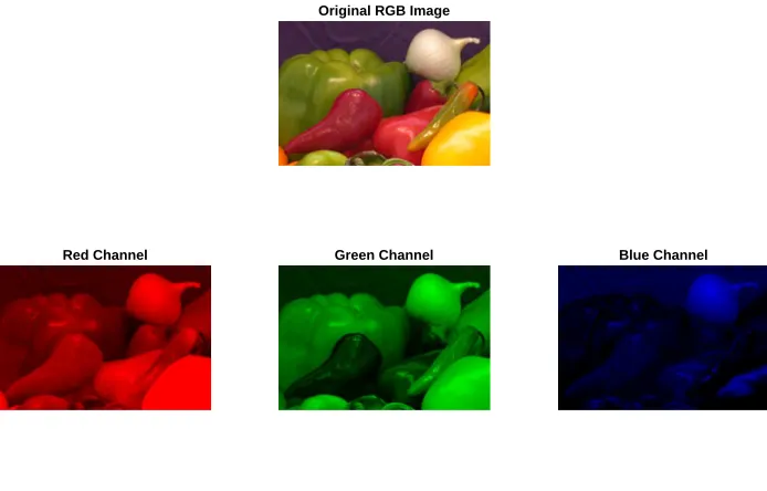
In the case of color images, each pixel in the matrix is an array of 3 values each

correspond-ing to color or brightness dependcorrespond-ing on the color map. The most commonly used color map is

the RGB space, where each value in the array represents the brightness level of the red, green,

(17)

Original RGB Image

Red Channel Green Channel Blue Channel

Figure 2.3: Image broken down to individual RGB channels.

Plenty of other color spaces exist, one of which is the Hue, Saturation, and Value (HSV)

space where the colors in the image are modelled to be similar to how humans perceive color.

Another commonly used color space in digital videos is the YCbCr, where visual information

is stored as values of Luminance (Y) and Chrominance(Cr and Cb). The pattern persists,

however, in that pixels in color images are usually composed of an array of 3 values.

Even though computers ”see” images as merely matrices, important visual information

about the image can be inferred from these matrices [8, 9]. For example, in natural scene

images, pixel values in a neighbourhood are highly correlated. Looking at the green channel

image in Figure 2.3, a random pixel in the middle of the onion on the top right part of the

image is guaranteed to have an adjacent pixel that has a value very close if not identical to it.

This maintains a consistent color gradient pointing towards the existence of an object within a

localized area in the image.

Another interesting property of images is that edges of objects could be deduced with a

sharp difference between adjacent pixels [8, 9]. As an example, in Figure 2.2, a vertical edge could be inferred from a sudden change of 0 to 127 and 0 to 255 in the pixel values in the first

and second columns of the image. The same is true in deducing horizontal edges in that there

(18)

Figure 2.4: Histogram of a sample image.

Traditionally, the pipeline for image classification is as follows: first, nfeatures from the

image is extracted, then thesenfeatures are combined to create an n-dimensionalfeature vector

which represents each image. Thisndimensional feature vector could be thought of as a point

in anndimensionalfeature space. Therefore, each image in the dataset exists as a point in this

ndimensional feature space.

Features with which to represent images are not only limited to edges and neighbourhood

pixel values, however, and research is being actively done on figuring out the best features to

use in representing an image [10–13]. Some of the most popular feature representations used

in computer vision are highlighted below.

2.1.2 Image Feature Representations

One of the more intuitive ways to represent an image is by looking at the raw pixel values

in the images themselves. After all, the pixels themselves contain information about color or

brightness. Information garnered from raw pixel values has been dubbedfirst-order statistics

(19)

First-Order Statistics

• Mean (average gray level intensity within the image)

¯

I = 1 N

N

X

i=1

I(i) (2.1)

• Median (middle gray level value when the gray levels are sorted)

Imedian =

n+1

2 th (2.2)

• Standard Deviation (amount of variation between the gray levels)

Isd=

v t

1

N−1

N

X

i=1

(I(i)−I¯)2 _(2.3)

• Skewness (measures of the asymmetry of the distribution of the histogram)

skewness=

1 N

PN

i=1(I(i)−I¯)3

q₁

N

PN

i=1(I(i)−I¯)2

3

(2.4)

• Kurtosis (measures the sharpness of the peak of the distribution of the histogram)

kurtosis=

1 N

PN

i=1(I(i)−I¯)4

q₁

N

PN

i=1(I(i)−I¯)2

4

(2.5)

where: I =Image matrix

N =Total number of pixels in the image

Second-Order Statistics from Gray Level Co-occurence Matrices

On the other hand, Haralick et. al. [15] developed another way of looking at the texture of

images by first creating a Gray Level Co-occurence Matrix (GLCM) and then extracting

infor-mation from this matrix. The concept is based on the assumption that the texture of the image

can be gleaned from the relationship of the gray levels have with each other within the image.

(20)

there would also be four different GLCM’s. To illustrate further, Figure 2.6 shows how a typical GLCM would look like for the image shown in Figure 2.5. (0,0) would be the number of times

the gray level value 0 had a neighbouring pixel whose value is also 0. (0,1) would then be the

number of times gray level values 0 and 1 were neighbours with each other and so on. Keep

in mind that the definition of ”neighbour” is a function of the direction to which the adjacent

pixel is located, as well as the distancedwhich defines the scope of the neighbourhood.

Figure 2.5: Image example for GLCM creation. Image referenced from [15].

Figure 2.6: GLCM reference table. (i,j) is the number of times pixel values i and j have been

(21)

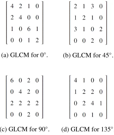
With this, Figure 2.7 shows the actual values of the four matrices given Figure 2.5.

(a) GLCM for 0◦. (b) GLCM for 45◦.

(c) GLCM for 90◦. (d) GLCM for 135◦.

Figure 2.7: GLCM values for a given image in Figure 2.5.

From these matrices, Haralick et. al. defined 14 textural features that can be used to

de-scribe the texture of an image. Some of the textural features are outlined below. The complete

list can be found at [15].

• Angular Second Momentum (measures the smoothness or uniformity of the image)

AS M= X

I1,I2

P(I1,I2)2 (2.6)

• Contrast (measures local level variations)

Contrast =−X

I1,I2

|I1−I2|2logP(I1,I2) (2.7)

• Correlation (measures pixel correlation in two different directions)

Correlation= X

I1,I2

(I1−µ1)(I2−µ2)P(I1,I2)

δ1δ2

(2.8)

• Inverse Difference Moment (measures the homogeniety of the image)

Homogeniety= X

I1,I2

P(I1,I2)

1+|I1−I2|2

(22)

2.2 Training a Classifier

The selection of features to represent an image is very important because the classifiers depend

on these features to make a decision on whether or not an image belongs to a particular class.

Usually, features are chosen such that there is a clear and distinguishable difference between images belonging in different classes. If for example the features chosen do not represent the image well (i.e. there is little variation between features of images belonging in different classes), then the classifiers would fail to be accurate.

After careful selection of the features, the next step is to train a classification algorithm.

Generally, each classification algorithm takes an input feature vector, performs a number of

operations on them, and then outputs a prediction for which class the input feature belongs.

Training a classifier then entails that the algorithm learns to adjust its parameters so that it could

output better predictions and differentiate between classes effectively. Some of the commonly used classification algorithms will be discussed in the next section.

With a huge enough database, a collection of the chosen feature vectors is used to create a

training set, avalidation set, and atest set. Typically, a dataset is split into around 70% training

set, and 15% for both the validation and the test set. From the names themselves, the training

set is used to train the classifier. The validation set is used to check how the classifier performs

during training, which would then indicate if training is sufficient or not. If so, then the model is saved for further testing. Otherwise, training will continue. Finally, the test set is used to see

how well the model generalizes into never before seen data.

During the selection of features, it is also important to consider how many features to use.

If too many features were selected, this not only increases the computational resources to train

(23)

excellent accuracy on the training set but fails to generalize on the validation or test set. In

other words, the classifier ”memorized” the distinguishing features on the training set but fails

on never before seen data.

2.3 Classification Algorithms

The following section outlines the different classification algorithms commonly used in im-age classification. Take note however, that these algorithms are common across classification

problems, not just image classification.

As was alluded to in previous sections, the training set is fed into a classification algorithm

that takes in an input feature vector and outputs a prediction for which class that particular

feature vector belongs to. Often, this output is a probability that each input belongs to classyi.

There are 2 types of classification algorithms which will be described below.

2.3.1 Unsupervised learning

Unsupervised learning is an umbrella term for algorithms which make predictions without

looking at the class labels of each feature vector. Because of this, unsupervised learning

al-gorithms do not have prior knowledge of how many classes there are in each dataset. These

types of algorithms are more powerful, however, in that they can usually generalize better with

completely new input. At the same time, these algorithms can point towards similarities and

differences among objects beyond their class labels. Although these algorithms would not be explicitly used in this research, a brief spiel for unsupervised learning algorithm is given for a

potential future application.

K-means

One of the most common unsupervised learning algorithms is the the K-means algorithm. This

algorithm attempts to cluster the dataset into K predetermined classes regardless of whether

there are actually K classes in the dataset or not. This is done by first randomly selecting K

(24)

Figure 2.8: K-means algorithm visualization. a) Unclassified data points. b) Initialization of

two centroids denoted by the red and blue ”x”. c) The data points are labelled according to their

proximity with the centroid. d) The centroids are adjusted to reflect the average of all points

belonging to its own class label. The data points are then re-labelled, based on proximity with

the new centroids. e,f) The process is repeated until no new data points are re-labelled to a

different class. Image taken from [16].

Anomaly Detection

An anomaly can be defined as an instance or an object that does not conform to what is deemed

”normal” [17]. In terms of finance and credit cards, detecting anomalies could be seen as

detecting fraudulent purchases. In the same context, apoint anomaly [18] is one instance of

fraud where a purchase has been made in a country different from where the owner is currently at. A contextual anomaly [18] on the other hand is when the user goes on a vacation to a

(25)

Figure 2.9: Point anomaly illustration

2.3.2 Supervised learning

In training a supervised classification algorithm, the class labels for each feature vector is

known to the classifier and it uses these class labels to compare its prediction to the actual

class label of each feature vector. Keep in mind that since we are dealing with classification

problems, the output of the algorithms takes on discrete values which pertain to the object’s

class label. And in some cases, the output of the algorithms is the probability that an object

belongs to a particular class. The difference between the output of the algorithm and the actual class label is usually represented using aCost Function.

In learning how to predict correctly, the goal of training classification algorithms is to

minimize this cost function. Since the output of the classifiers is often a probability, minimizing

the cost function entails that the classifiers output a probability as close to 1 as possible for the

correct class and as close to 0 as possible for incorrect classes. Say for example we have a

dataset with 5 classes, y ∈ [cat,dog,goat,sheep, f ish]. When given an image of a dog, we want the output predictions of the algorithm be [0,1,0,0,0] where the algorithm is absolutely

sure that the image is that of a dog, and not of anything else. Otherwise, a predictions of say

[0.4,0.3,0.2,0,0.1] means that the algorithm is unsure about the class label of the image.

In general, the process is that upon making a prediction, the cost function is calculated to

see how far offthe prediction is from the true value. The classifier then adjusts its parameters in such a way that wrong predictions are penalized and correct predictions are reinforced.

To elaborate further, the most common supervised classification algorithms are outlined

(26)

hθ(~x)=g(θT~x)= 1

1+e−θT_~_x (2.11)

hθ(~x)= g(θT~x)= 1

1+e−(θ1x1+θ1x1) (2.12)

g(z)= 1

1+e−z (2.13)

where:g(z)=sigmoid function

θ1, θ2 =parameters to optimize

A plot of the sigmoid function is shown in Figure 2.10. Notice that g(z) approaches 1 as

z → ∞, g(z) approaches 0 as z → −∞. Therefore, we can approximate thatg(z) outputs the probability that a feature vector~xbelongs to classy = 1. Conversely, the probability that the same feature vector~xbelongs to classy=0 is 1−g(z)

Formally:

P(y= 1|~x;θ)= hθ(~x)=g(z) (2.14)

P(y=0|~x;θ)=1−hθ(~x)=1−g(z) (2.15)

∴P(y|~x;θ)=[hθ(~x)]y[1−hθ(~x)]1−y (2.16)

For all training samples m, the product of all the probabilities shown in equation 2.16 can

be thought of as theLikelihood Function where it measures how likely that the input feature

(27)

L(θ)=

m

Y

i=1

[hθ(x~(i))]y

(i)

[1−hθ(x~(i))]1−y

(i)

(2.17)

The goal of training this particular classifier therefore is to maximize the likelihood of an

input belonging in classy= 1. Therefore, we need to find the values ofθT _{such that}

g(z)→1 fory=1 and

g(z)→0 fory= 0

This basically indicates that we want the classifier to be 100% sure in determining whether

an input belongs to classy= 1 or not. One of the ways that this could be done is viaStochastic Gradient Ascent:

θB θ+α· ∇θJ(θ;~x;y) (2.18)

where:α= learning rate

∇_θ =gradient of the loss function with respect to parameterθi

L(θ;~x;y)= likelihood function parametrized byθ

This gives a parameter update rule as follows:

θj Bθj+α((y( i)₋

hθ(x(i)))x(_ji) (2.19)

The learning rate determines how fast the algorithm learns by scaling the change in the

parameters up or down. A lower learning rate means that the parameters would update slower,

therefore increasing the time it takes to train the algorithm. However, if the learning rate is too

(28)

Figure 2.10: Sigmoid Function Graph. Image taken from [19].

Support Vector Machines

Whenm samples with n dimensions are plotted inton dimensional feature space, the aim of

Support Vector Machines(SVM) is to find an optimal hyperplane that separates one class from

another. The separating hyperplane is optimal in such a way that the closest points to the

boundary are at a maximum distance from said boundary. To visualize, five samples of class

cross and classcircle with features x1 and x2 were plotted in Figure 2.11. Even though both

of the red lines separates the two classes, it does not do so very well as opposed to the solid

line in the middle as this line has the maximum distance between the boundary and the closest

points from each class.

(29)

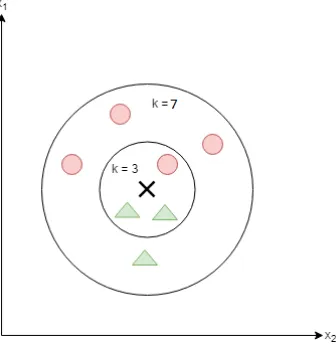
K-Nearest Neighbours

K-Nearest Neighbours is a supervised classification algorithm where a training sample is

as-signed a class via majority vote of the K nearest points in its neighbourhood. In Figure 2.12,

say we have an unknown point which is represented by theX in the middle. If we set K = 3, meaning we will only consider the 3 nearest neighbours of point x, we will assign classgreen

triangleto point x. However, if we setK= 7, we will assign classred circletox.

Figure 2.12: KNN Visualization.

A KNN algorithm withK =1 is simply known as the Nearest Neighbour algorithm(NN).

Decision Trees

Finally, a Decision Tree is a classification algorithm where each internal node represents a

discriminative decision between features and whose branches represent the outcome of the

decision. A class label is then assigned to the leaf node, which is result of the final decisions

as illustrated in Figure 2.13. As an example, if we have a classifier for fruits and our features

(30)

Figure 2.13: Decision Tree Visualization taken from [20].

Artificial Neural Networks

An Artificial Neural Network (ANN) is a machine learning algorithm that attempts to mimic

biological neural networks. The network is composed of an input layer, followed by hidden

or intermediate layers, and finally an output layer. Each layer further consists of neurons, or

nodes.

In the input layer, the nodes are simply each feature in the feature vector. Therefore, the

number of nodes on the input layer corresponds to the number of dimensions on the feature

vector. Each node on the hidden layer then takes the weighted sum of the output of the previous

layer and goes through anon-linear activation. Figure 2.14 shows the internal mechanics of a

neuron.

Figure 2.14: ANN Neuron illustration.

(31)

shown in equation 2.11. Keep in mind that since the previous layer is fully connected to the

current layer, each of the connections from one node to another would have its own

corre-sponding weight. The output of the sigmoid function would then be the input to the next layer,

with the same process repeated again. In addition to the weights of each of the connections, a

bias parameter is added per layer.

Finally, the output layer takes in the output from the last hidden layer and then performs a

different activation depending on the problem at hand. In multi-class classification problems, this activation function is often the softmax function, a generalization of the binary logistic

regression classifier.

fj(θT~x)=

eθT~xj

P

keθ

T_~_x

k (2.20)

where: k=number of classes

~x= input feature vector

The softmax function takes in an input vector xand outputs a value between 0 and 1 for

each class j. When concatenated, a vector of predictions ~f is produced for each input ~x.

The values in the vector of predictions sum up to 1. The output of the softmax function can

then be interpreted as the normalized probability that the input feature vector ~x belongs to a

particular class. Therefore, the nodes on the output layer matches the number of classes in the

classification problem. An illustration is provided in Figure 2.15

The algorithm learns by updating the weightsθand biasesbiwhich essentially dictates the

contribution of each input in the firing of the neuron. To adjust the weights, we first define a

new loss function suitable for multi-class classification called the Categorical Cross Entropy:

Ji =−fyi +log

X

j

efj _(2.21)

where: fyi = true class label

(32)

Figure 2.15: Artificial Neural Network architecture that attempts to classify an input with 4

features to one of three possible classes.

From equations 2.21 and 2.20 we get a cost function parametrized by the weightsθ:

Ji =−fyi +log

X

j

e

eθ T_~

x j

P

k eθ T~_xk

(2.22)

Take note that this follows the intuition for the loss function explained in the Logistic

Regression section where the loss is essentially the difference between the prediction of the algorithm and the true class label of each input. Since the aim is to minimize the cost function,

or to make the predictions as close to the true labels as possible, the weights are then adjusted

via a gradient descent method or variations thereof. To recap:

θ_B θ−α· ∇_θJ(θ;~x;y) (2.23)

where:α= learning rate

∇_θ =gradient of the loss function with respect to parameterθi

J(θ)= loss function parametrized byθ

For the first forward pass, the weights θ are initialized randomly and then updated using

equation 2.23. There are a few options available for when to update the weights. For instance,

one can choose to update the weights after one training sample has been fed forward to the

(33)

weights after a mini-batch of samples have been fed forward through the network (batch

gradi-ent descgradi-ent). Although stochastic gradient descent allows the weights to be updated right away

after a single sample, this often leads to huge fluctuations in the weights. Thus, batch gradient

descent is preferred by researchers because it takes into account more samples in updating the

weights. But at the same time, opting for mini-batches reduces computational complexity as

opposed to calculating the loss over the whole training set [21]. Once the entirety of the

train-ing set has had a chance to adjust the parameters, this is known as anepoch. Often times, one

epoch is not enough to sufficiently train a network. Thus, multiple passes through the training set is required to successfully create an accurate classifier.

There are better alternatives in updating the parameters however, one of which is the

Adap-tive Subgradient Method (Adagrad) [22]. The Adagrad optimizer introduces more variables

which adjusts the learning rates for each parameter depending on their past values. Larger

up-dates are done for infrequently appearing parameters and smaller upup-dates are done for frequent

parameters. The update rule then becomes:

θ_Bθ− √ α

Gt+

gt (2.24)

where:Gt = diagonal matrix where each diagonal element

is the sum of the squares of the past gradients with respect to parameterθi

gt = gradient of the loss function with respect to the parameterθi

=hyperparameter

= element-wise matrix multiplication operation

The advantage of using Adagrad is that manually tuning the learning rates for each

param-eters is no longer needed. Instead, the adjustments of the weights are dictated by their previous

values, which is contained inGt.

A variation of Adagrad calledAdadeltaalso computes adaptive learning rates for each

pa-rameter [23]. However, instead of taking the sum of the squares of the past gradients, Adadelta

(34)

mt =β1mt−1+(1−β1)gt

vt = β2vt−1+(1−β1)g2t

(2.25)

where:mt = estimate of the mean of past gradients (first moment)

vt =uncentered variance of past gradients (secont moment)

β1, β2 =decay rates (hyperparameter)

However, mt andvt are initialized to 0 and the first few forward passes tend to bias their

values close to 0 as well especially with low decay rates. To solve this problem, a bias corrected

first and second moments are used instead:

ˆ

mt =

mt

1−β₁vˆt =

vt

1−β₂ (2.26)

Finally, the update rule is computed as follows:

θ_Bθ− √ α

ˆ

vt+

ˆ

mt (2.27)

With enough training,θwould converge to a point where the loss function is at its minimum,

signifying that the model achieves its best predictions with the obtained values forθ.

2.3.3 Image Classification Metrics

One of the most intuitive ways to check the accuracy of the model is to measure how many

correct guesses it obtained on the test set. However, a dataset having a huge number of classes

calls for a more forgiving metric. For this reason, the top-5 error rateis used to consider the

(35)

Figure 2.16: Top 5 Error Rate illustration taken with permission from [25]. Actual class labels

are shown in larger text, and model predictions are shown with the colored bars indicating

confidence.

is the number of times where the true class label did not appear in the top 5 guesses of the

classifier. An illustration is shown in Figure 2.16.

For binary classification, theConfusion Matrix,F-Score,Recall, andPrecisionare all

use-ful metrics in determining model performance. The confusion matrix is a table showing the

number of true positives, true negatives, false positives, and false negatives predicted by the

model.

Actual class

Positive Negative

Predicted Class Positive True Positives (TP) False Positives (FP) Negative False Negatives (FN) True Negatives (TN)

Table 2.1: Confusion Matrix.

Precision is the ratio of true positive predictions to the total positive predictions outputted

by the model. A high precision indicates that the model could correctly predict positive classes

(36)

Recall= T P

T P+FN (2.29)

F-Score is a combination of the two:

F-score= 2· precision × recall

precision+recall (2.30)

F-score is a useful metric in cases where the dataset is severely unbalanced. For example,

say we are given a dataset that contains 90% positive cases and 10% negative cases. An

inef-fective classifier that simply guesses everything as positive would have a ”good” accuracy of

90%. However, the true performance of the classifier would be reflected on the precision and

hence, the f-score of the classifier.

2.4 Rock Image Classification

In the field of geology, image classification is not unheard of and has tremendous potential

ap-plications. For example, autonomous hyperspectral image classification has huge applications

in mapping unexplored surfaces [26, 27]. Also, classifying rock images garner significant

at-tention from researchers. For instance, Harinie et. al tested image classification algorithms on

four types of rocks: intrinsic igneous, extrinsic igneous, sedimentary, and metamorphic [28].

It was accomplished by extracting Tamura features [13] from a set of 50 images and then using

these as standard features for each class. Subsequent images are then classified by comparing

the basis features with the Tamura features of the input image. The image is then assigned to

the class with the minimum distance with the basis. Through this method, the authors obtained

(37)

As well, Mlynarczuk et. al. classified thin section images of nine different rock samples [29]. First order statistics were used as features for each image. The features were extracted in

four different color spaces namely RGB, HSV, YIQ, and CIELAB [30,31] to examine the effect of color spaces in automatically classifying each image. Using these features, the authors found

that the Nearest Neighbours and K-Nearest Neighbours algorithms performed best across all

color spaces, achieving an accuracy upwards of 96%.

Meanwhile, Shang and Barnes hand crafted 54 different features based on first order statis-tics and used three different classifiers (SVM, KNN, Decision Trees) to classify rock images baased on 14 different textures [32]. However, to help with efficiently choosing which features are more important than others, they employed a reliability based method for feature selection.

For each training sample, the reliability of a feature is given by its distance to the same feature

from other training samples belonging in the same class. Farther distances suggest that the

feature might not be a good indicator of class membership, and can therefore be omitted from

the feature set. The features are then ranked based on the reliability and only the topmreliable

features are selected. As well, the researchers used an Information Gain based ranking to rank

the features based on how well they separate data points with respect to their underlying class

labels. This is done by calculating the entropy of the class before and after taking a feature

into account and then measuring the additional information about the class that the feature

provides [33]. Again, the topmfeatures are selected.

Overall, the authors achieved the highest accuracy by using the top 20 features out of the

possible 54 with an SVM classifier. In using all 54 features, the authors did not see any

signif-icant increase in accuracy for the SVM. However, in both KNN and Decision Tree, the authors

obtained the highest accuracy by using 53 and 48 features respectively. Similar results are

observed when using Information Gain based ranking.

Ishikawa and Gulick takes a different approach in mineral classification, this time by using Raman Spectra instead of color images [34, 35]. The authors gathered Raman data from 13

different minerals and segregated them according to mineral group. A total of 190 spectra each with 765 dimensions were collected. To reduce the number of dimensions on the feature

set, the authors used Principal Component Analysis to map the features into a space where

(38)

plane polarized and cross polarized light with each pixel being labelled according to its mineral

content. The authors used raw pixel values on the RGB and HSV spaces as the features which

was then fed into an Artificial Neural Network with 1 hidden layer. The authors obtained an

accuracy of 89.53% when using the RGB color space, 87.5% in HSV and 87.45% using both

color spaces.

Finally, Singh et. al used a mix of first and second order statistics, Image Features

(percent-age of most common gray level, number of edge pixels, etc.) and Region Features to classify

textures of basaltic rock images into three classes [37]. In total, 27 features were selected.

Principal Component Analysis was again used to reduce feature dimensionality. An Artificial

Neural Network was also used, having 2 hidden layers and 15 and 20 nodes respectively. The

authors obtained an average classification accuracy of 92.22%

2.5 Convolutional Neural Networks

2.5.1 AlexNet and the Rise of ConvNets

The previous work that has been shown has a common thread: manually extract features and

build a feature set, try to optimize feature selection, and finally train a classifier. However,

recent developments in image classification has a more different approach. The idea is to automate the whole process and have an algorithm learn which features to extract and then

train a classifier at the same time. This method was first proposed by LeCun et. al. and has

been dubbed Convolutional Neural Network [38]. In their work, the authors developed the

LeNet-5 (Figure 2.17), a ConvNet that classifies hand written digits from the MNIST dataset

consisting of 60,000 training samples and 10,000 test samples. The method boasts an accuracy

(39)

More recently, ConvNets have risen to popularity because of the work of Krizhevsky et.

al. [25] in achieving unprecedented accuracy in the ImageNet Large Scale Visual Recognition

Challenge 2012 dataset [39]. The feat is impressive because the ImageNet dataset is composed

of 1000 different classes with a total of 1.2 million images in the training set and 200,000 images in the validation and test set. Also, the images are of different scales and often off -center objects. Obtaining very accurate results on this dataset translates well into classifying

real life natural scene images. Because of the success of Krizhevsky et. al., subsequent top

submissions to the contest used variations of ConvNets [40–43].

Figure 2.17: LeNet architecture taken from [38].

Figure 2.18: AlexNet architecture taken with permission from [25].

(40)

and the fully connected layer, both of which are going to be explained below. Finally, the

out-put layer is similar with the ANN where the outout-put is the probability of a feature set belonging

in a particular class.

ConvNets work in the same mechanics as the ANN in such a way that it also attempts to

mimic how the brain interprets images. Imagine for example how an infant would differentiate between shapes. One would imagine that that the edges of each objects are one of the main

factors in deciding shape. Over time, an infant learns that an object with four edges is a square,

and object with no corners is a circle, and so on. Then, in differentiating different objects, combinations of shapes, edges, as well as colors are taken into account. Thisobject has this

shape and thiscolor. The face of mommy and daddy havetheseshapes and their hair is that

color. And as children learn more shapes and more objects, the distinguishing features tend to

be more complicated.

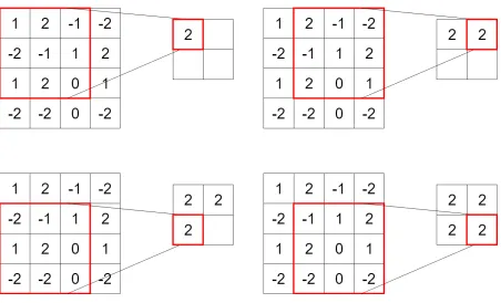
Convolutional Layer

At the core of ConvNets is the convolution layer. A convolution with an image is simply a

weighted sum of the pixels within the window size of the filter called the receptive field. To

illustrate, Figure 2.19 shows a 4×4 sample image convolved with a 3×3 filter with weights [1 1 1; 1 1 1; 1 1 1]. This simply results to a linear sum of all the pixels in the receptive field of

the filter. Then the window moves over to the next central pixel which fits the filter, also known

as thestride. In this example, the stride is 1. This process is repeated until the convolutions all

through out the image are exhausted, creating afeature map.

(41)

be 3×3×3, matching the depth of the input.

Figure 2.19: Convolution Demonstration.

There are a few things to consider with this process. When we convolved the 4×4 image with a 3×3 filter, the result is a 2×2 feature map. Increasing the receptive field size of the filter to 4×4 would then result into a 1×1 feature map. In the same way, if the receptive field size of the filter is decreased to 2×2, the result would also be a bigger feature map, 3×3 to be precise. However,paddingthe borders of the original image with zeroes (therefore increasing

the number of convolutions throughout the image) could result in an output image with the

same dimensions as the original.

The output of each filter would then be stacked on top of each other, creating a 3-dimensional

feature map. In general, the output of the convolution layer is a 3-D volume [H2 ×W2× K]

where:

H2 =

H1−F+2P

S +1 (2.31)

W2 =

W1−F+2P

(42)

F =Filter Receptive Field Size

P= Zero padding

S =Strides

The number of filters per convolution layer depends on the discretion of the researcher.

Even the most common networks employ varying numbers of filters per layer, and there is no

hard and fast rule on how many filters there should be per layer.

In this algorithm, the weights of the filters are learned through the same process as in

Artificial Neural Networks. A loss function is defined, and the weights of the filters are updated

using an optimizer as in equation 2.26.

Convolving images with specific filters create interesting feature maps that would be useful

for classification purposes. For instance, convolving an image with a Sobel Kernel produces a

feature map of vertical and horizonal edges in the image (Figure 2.20).

Similar to how nodes in ANNs are activated by a non-linear activation function, image

con-volutions are followed by an activation function as well. The most commonly used activation

function is the Rectified Linear Units (ReLU) where:

f(x)= max(0,x) (2.33)

The activation is simply a threshold at 0. A graph of the activation function is shown in

Figure 2.21. Variations of this activation function exists, one of which is the Leaky ReLU

which does not impose a hard threshold on 0, but instead lets linearly adjusted negative values

pass through. Another variation is ReLU(n) wherenis a maximum threshold arbitrarily chosen

(43)

Figure 2.20: Edge Detection with Sobel Kernels. Top: horizontal edge detection kernel.

Bottom: vertical edge detection kernel

(a) ReLU. (b) Leaky ReLU. (c) ReLU(n).

Figure 2.21: Rectified Linear Units activation function graph.

Pooling Layer

Convolutional layers are often followed by a pooling layer which reduces the dimensionality

of the input. The mechanism is similar to the convolution layer where a sliding window

prop-agates through the image. However, the output of the pooling operation is a choice between

the maximum pixel value within the window (Max Pooling), or the average of the pixel values

(Average Pooling). Going back to Figure 2.19, if the operation was instead Max Pooling, the

result would be Figure 2.22. The choice of pooling operation is left to the researcher, however,

(44)

Figure 2.22: Max Pooling.

The purpose of the pooling layer is to aggregate responses within a local area of the image.

On one hand, this reduces the number of parameters within the network. This provides two

benefits: reducing the computational complexity of training the network, and combats

overfit-ting by reducing the feature map. On the other hand, this operation brings a level of invariance

to positional changes within the image, meaning the exact position of pixels in the image would

matter less while preserving the structure of the whole image. Ultimately, this affords the clas-sifier some leeway in that regardless of where the object is in the image, the clasclas-sifier would

still be able to successfully recognize the image [44].

Fully Connected Layers

After a series of convolutions, activations, and pooling, the resulting 3D feature map is then

flattened, creating a 1-D vector of size H×W × K. This essentially creates the input for the hidden layers of an ANN, which comprises the last few layers of the CNN. Again, similar to

(45)

2.6 ConvNet Architectures

Over the years, different ConvNet architectures have been built and different intricacies have been placed to improve classification accuracy. The following section outlines the most popular

ConvNet architectures in current literature.

AlexNet

As was mentioned earlier, the work of Krizhevsky et. al. [25] jump started the popularity of

ConvNets in image classification. In particular, the authors achieved the best accuracy in the

2012 ImageNet Large Scale Visual Recognition Challenge (ILSVRC2012) [39] achieving a

top 5 error rate of 15.32%, while the second place holder achieved a significantly worse top

5 error rate of 26.17%. Their architecture composed of 5 convolutional layers activated using

the ReLU operation, and 3 pooling layers in between. There are three fully connected layers

after the convolutions containing 4096, 4096, and 1000 nodes respectively. The simplified

architecture is shown in Figure 2.23.

The Dropout layer before the fully connected layer is one of the major contributions of

Krizhevsky’s work. This layer randomly shuts offthe output of a hidden node during training. The probability that a node would be shut offis defined by thedropout rate, which is 50% in the case of AlexNet. Essentially, this process changes the architecture of the whole network

every time a new input is presented to the network. During testing however, all neurons are

activated. The overall effect of the technique is that it removes the reliance of neurons to one another, forcing the network to learn more complex features that would classify an image

correctly regardless of whether all neurons are firing or not [45, 46]. As a side effect, the training accuracy may be lower than validation accuracy when all neurons are activated.

Figure 2.23: AlexNet Simplified.

This network has over 62.3 million parameters to learn. Although that sounds like a

(46)

sification contest was achieved by fine tuning AlexNet [47]. Zeiler et. al. first deconstructed

AlexNet and visualized the activated feature maps after passing through each convolutional

layer in the network. The authors found out that the first layer extracts basic edges and edge

orientations, and deeper layers extracts more complex structures that are often class specific

(i.e. face of a dog, eyes, flower petals, etc.) [43]. Figure 2.24 shows sample feature map

activations in the different layers of AlexNet.

With this, the authors learned that the first two layers had innate problems within their

activations. The first layer extracts high frequency and low frequency information, but lacks

mid frequency information thus prompting the authors to reduce the receptive field sizes of

the filters in the first layer down to 7×7. Also, the second layer showed aliasing artefacts or blurred edges, which is indicative of subsampling in the images. To mitigate this, the authors

reduced the stride of the first layer down to 2. Finally, the authors achieved a top 5 error rate of

11.7%, a significant improvement from AlexNet’s 15.32% [43].

VGG

Inspired by the work Zeiler et. al. in decreasing the receptive field size of the first convolutional

layer in AlexNet, Simonyan et. al. decided to push the idea further by using only 3 × 3 convolutions in their network [48, 49]. By decreasing the receptive field size of the filters in

each layer, this also allowed the authors to create very deep networks.

Figure 2.25 shows the architectures Simonyan et. al. designed for the deep networks using

smaller convolutional filters. The authors tested 6 architectures in total, each with varying

depths.

On their own, all the networks performed better than AlexNet with the 11-layer network

achieving a top 5 error rate of 10.4% and the 19-layer network achieving 8.0%. Ensembling

(47)

(48)

Figure 2.25: VGG Architecture taken with permission from [48].

7.4% while achieving a top 1 error rate of 24.4% [47].

ResNet

Work done by He et. al found that in training very deep networks, the training accuracy seems

to approach a ceiling and then degrades rapidly [50]. They claim that this is not a problem of

overfitting on the training set, but that of unnecessarily adding depth to the network [41, 51].

To solve this problem, the authors introduced Residual Learning, where the output of a layer

(49)

Figure 2.26: Residual Networks Building Blocks taken with permission from [50].

The authors evaluated their hypothesis in 18, 34, 50, 101, and 152 layer networks using

the ImageNet dataset. The architecture of the 34-layer residual network is shown in Figure

2.27. The deeper networks simply appended more ResNet blocks and convolutional layers.

The authors achieved the best result in the 152-layer network with a top 5 error rate of 4.49%.

Combining the different networks in an ensemble, the authors achieved a maximum of 3.57% n the top 5 error rate, enough to win the ImageNet contest in 2015 [47].

Inception, InceptionV2, and InceptionV3

Stemming from previous work about improving classification accuracy with deeper and wider

networks [48, 51], it seems that the most intuitive way of achieving an even higher accuracy is

to go even deeper and wider [52]. There is a limitation, however. As more and more layers are

added to the network, the computational costs for training the classifier increases dramatically.

After all, the memory capacity of the GPU is very limited. To address this dilemma, sparse

connections in the fully connected layer or even in the convolutional layer must be introduced

[53]. Sparse connections reduces computational complexity by zeroing out most of the neurons

in the network. However, there is a trade-off: GPUs and CPUs are optimized for dense matrix calculations and using them for sparse matrix operations would have a detrimental effect to training duration. In fact, Liu et. al. explored the idea of Sparse Convolutional Networks and

managed to create a network with 90% sparsity. But, even with most of the parameters zeroed

out, the actual training times failed to reach the theoretical speed up times because of sparse

(50)

(51)

Szegedy et. al. then introduced the Inception Module (Figure 2.28) as an approximation

to a sparse structure all the while using dense matrices. The overall effect is deepening the network, and training less parameters at the same time. This is achieved by combining various

operations in each block, and concatenating the result of each filter to form a 3-D feature map

that has scale variance stemming from the different operations. In the case of the Inception Module, 1×1, 3×3, 5×5 convolutions were contained in a block, as well as 3x3 max pooling (Figure 2.28a). Zero padding has presumably been added so that all operations have the same

output dimensionality.

With adding these operations per block, the number of trainable parameters is sure to

in-crease. To remedy this, the dimensionality of the output volumes are reduced by adding 1x1

convolutions before the 3×3 and 5×5 convolutions (Figure 2.28b). The 1×1 convolutions operate on individual pixels, but extends through the depth of the 3D volume. As an

illustra-tion, if the 3D volume has dimensions 128×128x256 and 1×1 convolutions were operated on the volume, the output would be a 128×128×Kvolume whereKis the number of 1×1 filters used. As an added benefit, the Inception module follows the intuition that visual information

should be processed at various scales and then aggregated so that the next stage can abstract

features from the different scales simultaneously [52].

With the Inception module, the authors created GoogleNet which has 9 inception blocks

stacked on top of each other including 22 layers with trainable parameters. The architecture of

the whole network is shown in Figure 2.29. By ensembling 7 networks, the authors won the

2014 Imagenet classification contest with 6.67% top 5 error rate.

Operating on the same principle, different versions of the Inception module has been pro-posed by the author to optimize the networks further [55]. In [56], the authors used consecutive

3x3 convolutions to replace the 5x5 convolution in Figure 2.30 as well as widening the network

further by concatenating the results of operations with the same output size. Thus, using the

inception modules as building blocks, InceptionV2 and InceptionV3 was born. Upon training

and testing, both networks achieved 21.2% and 18.77% top 1 error rate respectively and both

exhibited improved top 5 error rates at 5.6% and 3.58% respectively.

Finally, the authors combined the principles of the Inception module with Residual

(52)

Figure 2.28: Inception Module taken with permission from [52].

to propagate through the input feature map for each block. This combines the best of both

worlds in that deep network degradation is adressed using Residual Learning, and computional

overhead reduction is tackled by Inception Modules. One of the many modules used by the

authors is shown in Figure 2.31. A complete list of the Inception-ResNet modules can be seen

in [55].

On its own, an Inception-ResNet network achieved a top 1 error rate of 17.8% and top 5

er-ror rate of 3.7%. Ensembling a ResNet, InceptionV3 and multiple Inception-ResNet networks

(53)

(54)

Figure 2.30: Inception V3 Module taken with permission from [56].

Figure 2.31: Inception-Resnet Module A taken with permission from [55].

DenseNet

With the seeming trend of making convolutional networks deeper while reducing trainable

parameters, Huang et. al. proposes a solution similar to that of ResNet but instead of only one

skip connection between layers, the DenseNet module has the output of all layers connected

to all other subsequent layers [57]. Figure 2.32 illustrates the DenseNet module. Within the

module, the output of layer x0 is taken as input of the rest of the layers x1−4. Similarly, the

output of layerx1is taken as input of the rest of the subsequent layers x2−4 and so on.

Although there are similarities with the Inception Module where multiple skip connections

(55)

varying depths and applied DenseNet modules (DenseNet-121, 169, 201, 264). In testing with

the ImageNet dataset, the authors obtained a top 5 error rate of 5.2% which is slightly worse

than the Inception Ensemble. However, their result is better than a stand-alone ResNet, while

keeping computational costs lower.

Figure 2.32: DenseNet Module taken with permission from [57].

MobileNet

Considering that mobile phones and embedded systems have way less powerful GPUs than

full computers, lightweight networks are needed to actually provide practical uses for image

classification algorithms. Because of this, Howard et. al. created MobileNet, a lightweight

network that is designed for mobile deployment [58]. To reduce computational complexity,

MobileNet splits a traditional convolutional layer into depthwise convolution and 1x1 point

wise convolutions:

The trade-offis that the accuracy of this model does not perform well against deep fully convolutional networks. In fact, in the ImageNet dataset, the maximum top-1 error rate that

MobileNet achieves is 29.4%, lower than Inception-ResNet by 11.4%.

2.7 Transfer Learning

With all these networks designed specifically to extract features on a huge dataset, a lot of

(56)

Figure 2.33: MobileNet splitting convolution layer into depth-wise convolution and

point-wise convolutions. Image taken from [58].

to a task that is fairly different from the original one with which the network has been trained [59–63]. The idea is that training the whole network and relearning the filters on a more

specific dataset would no longer be necessary. Instead, the weights of the filters from all the

convolutional layers would be kept the same. Only the softmax or output layer is left to be

trained, matching the output nodes with the target number of classes particular to the task

at hand. This is known as transfer learning. The advantage of using this method is that it

decreases computational costs associated with training very deep networks. A cluster of GPUs

would no longer be a requirement for training, and days or even weeks of training would no

longer be necessary.

Transfer learning is not limited to full Convolutional Networks only. In fact, since the

flattening the feature maps is a 1-dimensional vector, this could be viewed as the feature vector

of an image. This opens up the possibility of using a different algorithm as a final step in a classification problem. For instance, Razavian et. al. demonstrated this very idea in using a

pre-trained AlexNet as a feature extraction method and then using an SVM as a classifier for