Scholarship@Western
Scholarship@Western
Electronic Thesis and Dissertation Repository
8-17-2018 10:00 AM
Signal Identification In Discrete-Time Based On
Signal Identification In Discrete-Time Based On
Internal-Model-Principle
Principle
Jie Chen
The University of Western Ontario
Supervisor Lyndon Brown
The University of Western Ontario
Graduate Program in Electrical and Computer Engineering
A thesis submitted in partial fulfillment of the requirements for the degree in Master of Engineering Science
© Jie Chen 2018
Follow this and additional works at: https://ir.lib.uwo.ca/etd
Part of the Controls and Control Theory Commons, and the Signal Processing Commons
Recommended Citation Recommended Citation
Chen, Jie, "Signal Identification In Discrete-Time Based On Internal-Model-Principle" (2018). Electronic Thesis and Dissertation Repository. 5562.
https://ir.lib.uwo.ca/etd/5562
This Dissertation/Thesis is brought to you for free and open access by Scholarship@Western. It has been accepted for inclusion in Electronic Thesis and Dissertation Repository by an authorized administrator of
This work presents an implementation of a signal identification algorithm which is based on the
internal model principle. By using several internal models in feedback with a tuning function,
this algorithm can decompose a signal into narrow-band signals and identify the frequencies,
am-plitudes and relative phases. A desired band-pass filter response can be achieved by selecting
appropriate coefficients of the controllers and tuning functions, which can reject the noise and im-prove the performance. To achieve a result with fast transient characteristics, this system is then
modified by adding a low-pass filter. This work is based on the previous work in continuous time.
However, a discrete implementation should be much more practical. The simulation result shows
a good tracking of the original signal with minimal response to measurement noise.
Keywords: Signal Identification, Internal Model Principle, Frequency Estimation, Band-pass
First, I would like to thank my supervisor Dr. Lyndon J. Brown for his support and help. I began
to do a project with Dr. Brown in my sencond semester. After getting along with him for several
weeks, I felt like that he is the best professor I have ever met and a respectful inductor whom I want
to learn from. After I began my research, he definately gave me so many guaidances about how to
do research and how to learn from the previous work. No matter what questions I asked him, he
always explained to me patiently or guided me correctly. I really appreciate everything that he did
for me and for my research. He not only provides me the knowlege but also the courgrage to keep
doing research.
Last but not the least, I would also like to thank my families for their support both on matter
and spirit. Studying abroad alone is not an easy thing at first, it is them who gave me a lot of
Abstract ii
Acknowledgements iii
Table of Contents iv
List of Tables viii
List of Figures ix
List of Abbreviations and Nomenclature xiii
1 Introduction 1
1.1 Background . . . 1
1.2 Motivation . . . 2
1.3 Structure of this Thesis . . . 2
1.4 Main Contributions of this Thesis . . . 3
2 Review of Literature 4 2.1 Overview . . . 4
2.2 Control Theory . . . 5
2.2.1 Internal Model Principle . . . 5
2.2.2 Repetitive Control . . . 5
2.3.2 Short-Time Fourier Transform . . . 9
2.3.3 Gabor Transform . . . 10
2.3.4 Wavelet Analysis . . . 12
2.3.5 Hilbert Huang Transform . . . 14
2.4 Review of the Simple Adaptive Algorithm . . . 16
2.5 Conclusion . . . 18
3 Previous Work 20 3.1 Internal Model . . . 20
3.1.1 Previous work in continuous time . . . 21
3.1.2 Simple model in discrete time . . . 24
3.1.3 Alternative model in continuous time . . . 25
3.2 System with One Internal Model (Off-Line Tuning) . . . 26
3.2.1 Continuous time . . . 26
3.3 System with More than One Internal Model (Online tuning) . . . 28
3.3.1 Continuous time . . . 28
3.3.2 Linear dependence . . . 30
3.4 Summary . . . 30
4 Algorithm Development 31 4.1 Alternative Model in Discrete Time . . . 31
4.2 System with One Internal Model (Off-Line Tuning) . . . 32
4.2.1 Discrete time . . . 32
4.3 System with More than One Internal Model (Online tuning) . . . 35
4.3.1 Continuous time . . . 35
4.3.5 Linear dependence . . . 41
4.4 Improved Approach . . . 42
4.4.1 Method . . . 42
4.4.2 Low-pass filter . . . 42
4.4.3 Improved system . . . 44
4.4.4 Parameter calculation . . . 44
4.5 Summary . . . 46
5 Simulation Results and Comparison 47 5.1 Simulation and Comparison . . . 47
5.1.1 Signal to be identified . . . 47
5.1.2 Harmonic magnitude . . . 49
5.1.3 Band-pass filter . . . 49
5.1.3.1 Parameter calculation . . . 50
5.1.3.2 Frequency identification . . . 51
5.1.4 Low-pass filter . . . 55
5.1.4.1 Parameter calculation . . . 55
5.1.4.2 Frequency identification . . . 56
5.1.5 Accuracy comparison . . . 59
5.1.6 Effciency comparison . . . 60
5.2 Comparison to Other Algorithms . . . 61
5.3 Summary . . . 61
6 Conclusions and Future Directions 62 6.1 Conclusion . . . 63
A.2 S-Function(bandpass) . . . 78
Appendix B Matlab alternative approach code 80
B.1 IFD(lowpass) . . . 81
B.2 S-Function(lowpass) . . . 85
3.1 Coefficients of band-pass filter (continuous time) . . . 27
3.2 Denominator coefficients of band-pass filter and model (continuous time) . . . 27
3.3 Coefficients of model (continuous time) . . . 28
4.1 Denominator coefficients of band-pass filter and model (discrete time) . . . 34
4.2 Coefficients of band-pass filter (discrete time) . . . 34
4.3 Coefficients of model (discrete time) . . . 34
4.4 Calculation of ¯¯K . . . 34
4.5 Coefficients ofTlpden . . . 45
4.6 Coefficients ofTdeden . . . 45
5.1 Values of ¯¯Kin algorithm based on band-pass filter . . . 50
5.2 Values of ¯¯Kin algorithm based on low-pass filter . . . 56
5.3 Comparison of average frequency error among four algorithms . . . 59
2.1 Block diagram of original algorithm . . . 16
2.2 The phase diagram with two different magnitudes . . . 18
3.1 Simple tuning instantaneous Fourier decomposition block diagram . . . 21
3.2 Block diagram of continuous system with one internal model . . . 26
3.3 Block diagram of continuous system with more than one internal model . . . 29
4.1 Block diagram of discrete system with one internal model . . . 32
4.2 Structure of signal identification based on the internal model . . . 36
4.3 Bode diagram of band-pass filter . . . 37
4.4 Bode diagram of band-pass filter with notches . . . 38
4.5 Bode diagram of low-pass filter . . . 43
4.6 Improved structure of signal identification with model of DC content . . . 43
5.1 Block diagram of periodic signals generator . . . 48
5.2 Periodic signals . . . 48
5.3 Amplitude of first and second set of harmonics . . . 49
5.4 Frequency identification for first fundamental component of proposed tuning function 51 5.5 Convergence of the first and second component of band-pass tuning function . . . . 52
5.6 Convergence of the first and second component of continuous implementation . . . 53
5.7 Frequency identification for first and second component of proposed algorithm . . . 54
5.8 Fast Fourier transform of input signal and error in proposed algorithm . . . 54
5.12 Input, output and error in alternative algorithm . . . 58
Nomenclature
HHT Hilbert Huang Transform
¯¯
K1pq,K¯¯2pq Feedback controller gains in this work
pq Small real number
ˆ
ωp Estimated frequency
ωc Fudamental frequency
φ Relative phases
d Signal
G Tuning Function
K1ccpq,K2ccpq Continous-time Feedback controller gains in another previous work
K1cpq,K2cpq Continous-time Feedback controller gains in previous work
K1d pq,K2d pq Discrete-time Feedback controller gains in previous work
Ka Tuning Gain
pωq qthFrequencywithpthharmonic
Tbpn Transfer function of bandpas filter with notches
Tbp Transfer function of bandpas filter
TLpn Transfer function of lowpass filter with notches
TLp Transfer function of lowpass filter
v Noise
x1pq, x2pq State spaces states
AFC Adaptive feedforward cancellation
ASTFT Adaptive Short-Time Fourier Transform
DFT Discrete Fourier Transform
EKF Extended Kalman Filter
EMD Empirical Mode Decomposition
FD Frequency discriminator
FM Frequency modulated
FT Fourier Transform
IFD Instantaneous Fourier Decomposition
IMF Internal Model Function
IMP Internal Model Principle
STFT Short-Time Fourier Transform
TFR Time-frequency representation
TPAS Time-phase amplitude specture
VVS Virtual variable samplings
Introduction
1.1
Background
Signals are widely used in our life, such as military, radar, satellite, commercial field and
commu-nication. In signal processing field, including communication, the frequency of a sinusoidal wave
needs to be identified. When it comes to disturbance cancellation and signal estimation problems,
these signals can be modeled as linear combinations of sinusoidal waves, which has become a
pop-ular subject since they are predictable and periodic. This issue occurs in musical pitch tracking,
computer disk drives and continuous casting of steel.
It is usual to predict signals based on their past values, especially when their characteristics
vary slowly. Specifically, in control, communication and mechanical research fields, signals can
be represented by:
d(k)= n
X
p=1
mp
X
q=1
Apqcosφpq(k)+v(k) (1.1) where
φpq(k)= q k
X
i=1
vis noise and the signal is the sum ofntime-varying waves composed ofmpharmonics each. It is
assumed that the amplitudes vary slower than the reciprocal of the frequenciesqωp.
1.2
Motivation
In real life, almost all events involve signals. However, the vast majority of collected signals
contain noises or are the mixture of several signals. Due to external environmental interference,
it is inevitable that noise is always mixed in signals during signal acquisition and transmission
process. And the noise is an important factor affecting the target signal detection and identification performance, especially in some high-precision data analysis. Even a very weak noise may have
a tremendous impact on the analysis result. In order to denoise in the signal processing, signal
recognition is the first step which also has become a very important discipline. Instantaneous
frequency has been a classical issue in signal processing and system controlling fields.
The research of speech recognition technology is a hot topic in the modern era. The speech
recognition system has entered into people’s life extensively. For example, the speech recognition
system of vehicle instrumentation brings great convenience to people. The human-machine voice
communication has always been an urgent desire to achieve. After obtaining the voice signal, it is
necessary to identify the speech sound out of the mixed signal. A similar problem is encountered
in the control field where it is desired to perfectly track reference signals or reject predictable
disturbances. Control algorithms that adaptively achieve this goal can be seen to perfectly identify
either the disturbance and/or reference signal. So, identifying this signal is the very first and main step of all of these procedures. In this work, these algorithms will be turned from signal processing
problem to control problem by using a tuning function to control the process. Our goal is to get
the algorithm that can work on audio signals at 20kHz.
1.3
Structure of this Thesis
In Chapter 2, the relative literature is reviewed.
In Chapter 3, the previous work is shown.
In Chapter 4, the algorithm is introduced in detail.
In Chapter 5, simulation results verify the feasibility of the algorithm and by comparing it with
other methods, the pros and cons of this algorithm are clearly shown.
In Chapter 6, a brief conclusion and the proposing work in the future are illustrated.
1.4
Main Contributions of this Thesis
The main contributions of this thesis are assigned as follows:
First, an improved method for the calculations of the final 4 parameters for the algorithm
pre-sented in [32] were developed.
Second, the implementation of the real-time algorithm proposed by Mohsen is successfully
converted to discrete time, which is much more easier for a computer to process, and the result
shows that it uses only half of the computational power of previous work.
Compared with the related works before, this thesis finds out a way to completely identify
Review of Literature
2.1
Overview
In this chapter, a literature review of related background of our research is presented in both basic
control field and signal processing field.
At present there are many techniques for identifying or canceling a periodic signal. Most
of them can be classified as either time-frequency representation-based methods or filter-based
methods. The main approaches will be analyzed in this chapter.
Methods of signal identification in signal processing field include: Fourier Transform, which is
the most traditional technique, wavelet analysis, Gabor analysis and the approaches that are based
on adaptive notch filter and output regulation. Another approach that has been widely used and
discussed is Hilbert-Huang Transform (HHT).
When it comes to control field, the same problem can be converted to signal tracking or
dis-turbance rejection. Two of the methods of this problem are repetitive controller and adaptive
2.2
Control Theory
2.2.1
Internal Model Principle
It is known that Internal Model Principle(IMP) was proposed by Francis and Wonham in 1976 [12].
This principle states that the internal model, which is a dynamic model of the disturbance, is placed
in a stable feedback loop to cancel the disturbance or track reference signals. One interpretation
is that the linear feedback system will cancel a particular frequency if the controller has the gain
of infinity at that frequency. Sinusoidal disturbances have drawn an amount of interest both in
estimation and in rejection issues. In this case, the controller must have a pair of poles on the
imaginary axis in the s-plane at a location corresponding to the frequency of the disturbance.
Internal model is used in order to supply transmission zeros.
In discrete time, the controller’s poles at e±jωpq make the controller’s gains atω
pq infinite. In
order for the algorithm to be stable, the input at these frequencies must be zero. Further, the gain of
the plant needs to be known sufficiently accurate to ensure negative feedback. IMP control suffers significant degradation of performance unless the frequency of the signals is known perfectly. Also,
small errors in this model can lead to significant degradation in effectiveness.
2.2.2
Repetitive Control
The basic idea of repetitive control comes from the internal model principle in control theory [15].
Repetitive control is used specifically in dealing with more complex periodic signals than a simple
sinusoid. Fourier Series theory states that any periodic signal can be represented by a sum of
sinusoids composed of a fundamental signal, i.e. a sinusoid with the same period as the periodic
signal, and the fundamental harmonics,i.e. sinusoids whose frequencies are integer multiples of
the fundamental. Thus, in continuous time, a perfect model of any periodic signal with period
T would be a model with its poles at 2jπ/T. This infinite number of poles can be generated by
a feedback loop about a pure delay of T. Typically, in order to stabilize the system, a low-pass
energy modes to move to the left of the imaginary axis, and increasing the stability of the closed
loop system. In our work, as an alternative, we keep the poles of the controller on the 2jπ/T
[15, 48]. The internal model principle is to embed a dynamic model of the system’s external
signal into the controller, and a mathematical model of the external input signal is included in a
stable closed-loop system. This can ensure a high precision of the feedback control system. The
repetitive controller is actually a cycle-by-cycle superposition of the input signal. When the input
decays to zero, the output still repeats the same signal as what it is during the previous period. If
the repetitive controller is placed in the forward channel of the control system and the input error
exists, the output of the repetitive controller will increase periodically until the error is completely
eliminated, that is, no-error-tracking can be achieved. This method is effective for periodic signal tracking, disk drives [8, 14], satellite control [4], servo hydraulics [47], robotic manipulators [9],
etc.
However, due to the existence of the pure delayesT orz−N in the repetitive controller, its output is delayed by T or N beats with respect to the input. Therefore, in the transient process, the
repetitive controller can only respond after delayingN beats. However, it is difficult to stabilize a large number of marginally stable poles and thus a low-pass filter is needed for stabilization. Also,
the convergence is very slow and the system may converge to a local minimum.
In [15], a model to generate periodic signal is implemented into the closed-loop system to
achieve asymptotic tracking. To stablize the system, a low-pass filter is added as an appropriate
proper stable rational function. A synthesis algorithm is developed by using state-space approach
and factorization approach. This algorithm can also be implemented in a non-linear system.
In [48], the paper uses repetitive control schemes to track periodic signals with unknown or
slowly varying period. Although the signal to identify is in continuous time, the author uses a
recursive scheme in discrete time.
In [50], a modified repetitive-control system is used to improve the disturbance rejection
per-formance. The system is composed of two subsystems. The first subsystem is used to reduce the
In [27], a frequency adaptive discrete Fourier transform(DFT) based repetitive control(RC)
scheme for dc/ac converters is presented. Different from the traditional one, this scheme is not that sensitive to frequency fluctuation. In this paper, the virtual variable sampling(VVS) method
is used to enable the DFT-based selective harmonic RC to be frequency adaptive. To decrease the
off-order harmonic and halve the number of sampling delay in the DFT filter, an offorder harmonic DFT filter is used.
2.2.3
Adaptive Feedforward Cancellation
The method using adaptive feedforward cancellation(AFC) was first proposed by M Bodson, A
Sacks and P Khosla in [2], and is widely used [30]. Instead of using the control scheme based on
the internal model principle, this method is based on the phase-locked loop which is widely used
in frequency modulation in communication systems. It can not only reject the certain frequencies
but also reduce higher-order harmonics. However, this algorithm is not reliable since it needs to
calculate the gain of every frequency, and the number of frequencies to identify is also limited.
Two methods are presented in [1] to reject the sinusoidal disturbances with unknown frequency.
In the indirect approach, the frequency is estimated by an adaptive notch filter and then the result
is used in a separate algorithm to cancel the disturbance. However, in the direct approach, the
estimation and cancellation of frequency is carried out simultaneously. The convergence is ideal
for the direct algorithm but not the indirect one, while the indirect one has larger capture region for
the parameter estimates. Thus, each one has its own benefit. The direct approach is also used [37]
2.3
Signal Processing
2.3.1
Fourier Transformation
Fourier Transformation(FT) [3] is a traditional signal processing method in pure frequency domain.
It uses the original function with the superposition of complex sine components with different frequencies. The Fourier spectrum can be written as:
x(t)=
∝
X
i=1
aiej
R
ωidt
From the Fourier Transform formula, we know that to get the Fourier transform (spectrum) of
a signal, we must take an infinite period of time (−∞,+∞), that is, we must get all the informa-tion from the time domain. However, if you want to use the spectrum to describe the signal, no
matter how short the signal is, you need to describe it in the entire frequency domain. The Fourier
transform cannot give you the spectral information in a certain time period [t1,t2], which, however,
is often of great interest to us. For music signals, we often care about what and when frequency
notes are sent out. For seismic signals, we are concerned with what frequencies occur in the spatial
locations. These signals are all non-stationary signals. Their characteristics in the frequency
do-main vary with time. So, the characteristics of the frequency dodo-main of the signal at any moment
are very important, and we cannot completely separate the time and frequency domain. That is,
the Fourier transform has no locality. It is only applicable to deterministic signals and stationary
signals.
Due to the lack of temporal local information, there is a serious shortage of Fourier frequency
analysis for time-varying signals and non-stationary signals. It cannot tell us which frequency
occurs in which time, and cannot represent the distribution of the signal spectrum at one moment. If
the signal changes within a small neighborhood of a certain moment, the entire frequency spectrum
of the signal will be affected. However, the change of the frequency spectrum cannot fundamentally determine the temporal position of the change and the severity of the change. The time domain
reason is that the trigonometric basis of the Fourier transform is global, and its localized nature
is not that good. So, we can only obtain the entire spectrum of the signal, and it is difficult to determine the local characteristics of the signal in any small range in any limited frequency band.
Also, this method is quite sensitive to noise [46].
2.3.2
Short-Time Fourier Transform
To obtain the information of when these frequencies occur and the amplitude of the instantaneous
frequency at each time, we need time-frequency analysis. Hence, Short-Time Fourier
Trans-form(STFT) is put forward [39]. The signal x(t) is quasi-stationary, and STFT forx(t) is
Sx(t, ω)=
Z +∞ −∞
x(τ)h(t−τ)e−jωτdτ
whereh(t) is the analysis window. The window function is used to divide the whole process into
small processes. Each of them are approximately stationary. Then, we use FFT to analyze every
segment and we can know what and when frequency occurs. However, the width of this window
has to be determined in advance. If the window is too wide, the analysis in time domain is not
ac-curate enough; if it is too narrow, the accuracy will decrease in frequency domain. Obviously, the
width of the window can vary to improve analysis of non-stationary signal. Unfortunately, the
win-dow is fixed in one STFT process. Also, this method suffers from poor time-frequency resolution. Thus, it is not an ideal method of signal identification. The adaptive short-time Fourier
trans-form(ASTFT) was proposed which avoids the worst of the disadvantages of STFT. ASTFT uses an
adaptive window to achieve better time-frequency representation(TFR). In addition, a post-ASTFT
peak-tracking algorithm further improves the performance by following the continuous ridge in the
time–frequency plane and removing the spurious deviations. The algorithm is constructed under
a statistical detection and estimation framework and is an approximate maximum-likelihood
of frequency-modulated(FM) signals over the STFT and the frequency discriminator(FD) by 4–16
dB at the expense of higher computational and storage cost [25]. In this paper, the author selected
a length-N (N odd) unit-energy Hamming window as the base window, and the total cost of the
whole Instantaneous frequency estimation(IFE) is
N 2N+8 log2N+40+
7FLOPs/out put
However, the additional cost can be justified in many situations.
In [52], STFT is used to obtain time-phase amplitude spectra(TPAS) which can describe a
non-stationary signal. A modified STFT is firstly used to tune the amplitude, initial phase and
instantaneous phase distribution of the real signal as functions of time and frequency. Then, TPAS
can be calculated by these functions.
2.3.3
Gabor Transform
In order to solve the locality problem, in 1946, Dennis Gabor proposed the concept of "window
Fourier transform", namely Gabor transform. Window Fourier transform or Short Time Fourier
Transform can be expressed as
X(t, ω)=
Z +∞
−∞
x(s)g(s−t)e−jωsds
Define the base function as
ψt,ω(s)=g(s−t)ejωs
when t and ω vary, it constitutes a family which can be considered as a kind of ’basis’. g(s)
represents a window function, such as Hanning, Hamming and Gaussian windows. When we use
Gaussian window function, for example:
g(x)=π−14e−
The transform we get is called Gabor transform:
Tgaborf (t, ω)=π−14 Z +∞
−∞
f(s)e−(s−21)2e−jωsds
The window of Fourier transform or Short Time Fourier Transform(STFT) is the key to achieve
the local analysis. The scale of the window is a representation of the degree of locality. When the
window function is a Gaussian window, it is generally called a Gabor transform. The reasons for
choosing the Gaussian window are:
1) The Fourier transform of the Gaussian function is still a Gaussian function, which makes
the inverse Fourier transform become localized with the window function; and at the same time it
embodies the localization in the frequency domain;
2) Heisenberg uncertainty principle comes from quantum physics. It says that the position
and the velocity of a particle cannot both be identified at the same time. The uncertainty in the
postition times the uncertainty of velocity of a particle must be less than Planck’s constant. But
you can convert position and velocity to potential energy and connectic energy. So the product of
uncertainty of potential energy and connectic energy will be less than Planck’s constant. Potential
energy and connectic energy can be converted to time and frequency respectively. According to
the Heisenberg uncertainty principle, the area of the Gaussian function window has reached the
lower bound of the uncertainty principle, and it is a function that minimizes the area of the time
domain window,ie, the Gabor transform is the optimal STFT.
Note that the formula output of STFT has two independent variables, time tand frequencyω,
ie, it is a time-frequency analysis. However, once the window function is selected, the shape of the
time-frequency window remains unchanged, and the inherent relationship between the frequency
and the window width is cut off. The Gabor transform essentially is a single resolution analysis. The Gabor transform can achieve the purpose of time-frequency localization: it can provide the
whole information of the signal and can provide the information of the intensity of the signal’s
be provided at the same time. Gabor transform has been used in detecting diabetic retinopathy
[34], texture segmentation [16], and defect detection [21].
Gabor transform solves the problem of local analysis to a certain extent, but it is still difficult to obtain satisfactory results for catastrophic signals and non-stationary signals. That is to say, Gabor
transform still has its serious defects.
1) The size and shape of Gabor transform’s time-frequency window remain the same, only
the position changes. In practice, it is often desired that the size and shape of the time-frequency
window will change with frequency, because the frequency of the signal is inversely proportional
to the period. The high frequency part needs a relatively narrow time window to improve the
resolution. In the low frequency part, it is hoped that a relatively wide time window can be given
to ensure the integrity of the information. In short, an adjustable time window is desired.
2) The basis functions of Gabor transform cannot be orthogonal. For fear of losing information,
non-orthogonal redundant bases must be added in signal analysis or numerical calculation, which
increases unnecessary calculation and storage. That is, regardless of the study of low-frequency
components or high-frequency components, the width and height of the time-frequency window
used by the Gabor transform does not change, which is unfavorable for studying higher frequencies
or lower frequencies.
As for transient signals, multi-window discrete Gabor transform(M-DGT) is applied in [13].
Due to the balance of the width of analysis window and frequency resolution as well as time
reso-lution, two spectra are combined by geometric average. It shows higher time–frequency resolution
than that obtained when only the single analysis window is used in the traditional discrete Gabor
transform.
2.3.4
Wavelet Analysis
The concept of "wavelet" was proposed by French geologist J. Morlet in the study of the
distribu-tion of subsurface rock oil reservoirs in the 1980s and was successfully applied in geologic data
attenuation properties [31]. In 1987, Mallat proposed the idea of multi-scale analysis and the
Mal-lat algorithm [29], which unifies the construction of various concrete wavelet functions proposed
before this. The wavelet transform inherits and develops the localization idea of Gabor transform,
and overcomes some defects of Fourier transform and Gabor transform at the same time. The most
important is that the wavelet transform gives an adjustable time-frequency window. The width of
the window changes with frequency. When the frequency increases, the width of the time window
automatically narrows to improve the resolution. Using wavelet analysis is like using a camera
with a zoom lens, and it can show us any detail.
Define signal f(t)∈ L2(R), its Continuous Wavelet Transform (CWT) can be defined as
Wf (a,b)= 1
√ |a|
Z +∞ −∞
f (t)Ψ t−b
a !
dt
It can be seen that the wavelet transform of the signal f(t) is a binary function. It can also be seen
formally that the wavelet transform of the signal f(t) is essentially the weighted average of
original f(t) byψa,b(t) neart=b. This reflected the change speed of f(t) with the standard of ψa,b(t). In this way, the parameterbrepresents the time center or time point of the analysis, and
the parameter a represents the size of the nearby range centered on t=b. Therefore, the parameter
ais generally referred as a scale parameter (i.e.,ωin the Gabor transform), and the parameterbis
a time center parameter (i.e.,tin the Cooper transformation). So, wavelet transform is also a
time-frequency analysis.
The advantages of wavelet transform compared to STFT are obvious:
1) Since the wavelet mother function ψa,b(t) are equivalent to window function, the window
width is variable. So, the contradiction between time resolution and frequency resolution are better
resolved. Its law of change makes the wavelet transform has excellent localization characteristics,
and it is very effective for analyzing catastrophe signals and singular signals. It fully embodies the idea of constant relative bandwidth frequency analysis and adaptive analysis;
er-ent frequencies, and use different step size of the space-time domain corresponding to the size of the frequencies. Any minute details of the object can be continuously focused. This method has
great significance in spectrum analysis;
3) It is not required that the wavelet transform base is orthogonal. The product of time width
and frequency width is small, and the energy of the spread coefficient is more concentrated. However, the selection of wavelet bases is a very difficult thing. In some cases, in order to achieve their desired separation effect, the researchers also need to make the appropriate wavelet base according to a particular research. More importantly, this method is very redundant, that is,
the data is highly repetitive. But this transformation does not actually get rid of the limitations of
Fourier transform, it is a window adjustable Fourier transform, the window of the signal must be
smooth. In addition, the wavelet transform is non-adaptive. Once the mother wavelet is selected,
in the entire signal analysis process can only use this one wavelet base. This method is suited for
a slowly-varying signal.
2.3.5
Hilbert Huang Transform
Traditional Fourier analysis uses a series of trigonometric basis functions to orthogonaly compute
signals. However, for non-stationary signals, such as signals with varying frequencies, the Fourier
spectrum we obtained is only the average of the frequencies over a certain period of time and cannot
accurately describe the change in frequency-time domain. The Hilbert–Huang Transform(HHT)
was developed by N.E.Huang. It is a new method of self-adaptive time-frequency domain analyses,
which can eliminate human factors and is suited for non-stationary and non-linear analysis. The
Hilbert spectrum can be written as x(t) = Pn
i=1ai(t)ej
R
ωi(t)dt. Compared with Fourier transform,
it can be noticed that Hilbert transform is the extension of Fourier transform and HHT has more
general meanings.
Intrinsic mode functions (IMF) are narrow band components of a signal that represent the
indi-vidual oscillation modes in the signal. Since most signals are not IMF, a method called Empirical
instan-taneous frequency can be obtained after doing Hilbert transform to each IMF. Since instaninstan-taneous
frequency can only be applied to mono-component signals with a zero mean which does not
typ-ically exist in practical signals [19] [18], EMD has the ability to decompose a multi-component
signal.
The Hilbert transform gives a mathematically precise way of defining instantaneous frequency.
Unfortunately, this definition only agrees with our intuitive understanding when applied to narrow
band signals. Thus, it is desired to decompose signals into a sum of narrow band signals before
applying the Hilbert Transform. Also, HHT cannot separate frequencies which are closely located.
This will become a severe problem in power systems because the frequencies of oscillations
typ-ically distribute in a narrow band [24]. Third, the end effects of EMD makes the results on both ends of the data set meaningless. Last but not least, HHT is based on local characteristics which
makes it sensitive to not only signal dynamics but also noises [51].
To improve the end effects in EMD, mirroring approach [22], least square polynomial extending [38], constrained cubic spline [23] are proposed. By applying EMD with masking techniques,
which is adding a masking signal, the mode mixing can be improved [11][10][42][26]. Using
ensemble empirical mode decomposition(EEMD) can also solve this problem [49].
First of all, for steady signals or signals that contain less frequency components, HHT can
help us obtain good effect of decomposition and analysis. However, for signals which are non-stationary, more random, and cross-aliasing frequency components, the analysis results are not
good enough. Even if HHT is used to denoise, you still cannot tell the noise or useful signals. In
conclusion, the basic theory is still immature and needs to be improved and the sieve method does
not have a theoretical basis.
HHT has been applied to power quality analysis in [43] and oscillation analysis in power
sys-tems [41]. In [44], HHT is also used to analyze terahertz spectra in order to improve the state-of-art
detection sensitivity of inconspicuous spectral fingerprints for materials with low concentrations
and remote sensing. In [51], a preliminary result of an extended Kalman filter (EKF) method to
text text text text text text ( )
d t e t( )
+ + + + − u ( ) G s , n n m IM 1,1 IM 2 2 1 ˆ ( ) s s +
2 2
1
ˆ (2 )
s s +
2 ˆ 2
( n n) s s + m
1,2 IM 11 u 12 u n nm u
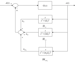
Figure 2.1: Block diagram of original algorithm
Since the IMFs are not orthogonal, the energy leakage is severe. In [20], three orthogonal
techniques are used to obtain the completely orthogonal IMFs. The orthogonal IMFs can produce
a more faithful representation of earthquake accelerators than the Hilbert spectrum and the Hilbert
marginal spectrum.
2.4
Review of the Simple Adaptive Algorithm
The original algorithm is processed in continuous time domain. An internal model of the signal
can be presented in state-space form:
˙ x1 ˙ x2 = 0 ω
−ω 0
u=
0 1
x1
x2
The input signal isd(t)= Acos (ωct+φ), whereωc is the true disturbance frequency andφis the phase. Thus, in steady states, ifω∼ ωc, we have:
e(t)=Aesin (ωct+ϕ)
x1(t)= Asin (ωct+ϕ)
x2(t)= Acos (ωct+ϕ) whereA= KfAe
ω2−ω2
c, andϕis the phase ofe.
The phase diagram of x1and jx2would show
|x1(t)+ jx2(t)|=
q
x21(t)+x22(t)=|A|
θ=∠(x1(t)+ jx2(t))=ωct+ϕ
The frequencyωc can be identified by the differentiating:
dθ dt =ωc
-2.5 -2 -1.5 -1 -0.5 0 0.5 1 1.5 2 2.5
x1
-2 -1.5 -1 -0.5 0 0.5 1 1.5 2
x2/wc
Figure 2.2: The phase diagram with two different magnitudes
ωc = ddtθ
= ω(x2
2+ω2x21−Kfex1) x2
2+ω2x21
= ω− Kfex1 x2
2+x 2 1
Up to here, we showed how the rotating speed of the circle in Fig. 2.2 can be used to solve the
unknown frequency.
2.5
Conclusion
Comparing wavelet transform, Gabor transform, and Fourier transform, we find that the Fourier
transform has no locality; the Gabor transform has locality, but has some shortcomings (as
de-scribed above); and the wavelet transform not only has locality, but also the scale parameteracan
change the shape of the spectrum structure and the window, and plays the role of “zoom”. So the
wavelet analysis may achieve the effect of multi-resolution analysis. From the theoretical develop-ment process of the signal analysis method, it can be seen that the Fourier analysis is particularly
Previous Work
3.1
Internal Model
Brown and Zhang [6, 7] presented an algorithm for identification of periodic signals with uncertain
frequencies. This approach is based on the internal model principle of control theory. An adaptive
internal model of a sinusoid is incorporated in a feedback loop to achieve the goal for disturbance
rejection and frequency estimation. The stability of the algorithm is proved in [7] by employing
the singular perturbation theory and averaging theory. The motivation of this algorithm is from the
realization that the actual frequency error can be inferred from the states of an internal model and
the feedback error by using a nonlinear mapping function. This adaptation method is very similar
to Hsu’s [17] update law but the normalization now comes inherently instead of as a modification
to Regalia’s algorithm [40]. This algorithm has already been applied on several applications, such
as musical pitch tracking[57], audio signal decomposition [28], power systems [56], sound and
vibration control [5] and dynamic resistance measurement in spot welding [45].
In [5], although excellent disturbance rejection has been achieved, the system is stable only
when the disturbance frequency varies in a small range. This will cause a problem for systems
having a large phase variation (exceeding 180) over the range of the frequencies of interest, This
+ -+ + + u d t
G s e t
2 2
1 s s
2 2
1 2 s s
2 2
q
s sp
. . . cpq u 11 c u 21 c u 11 c IM 21 c IM cpq IM
Figure 3.1: Simple tuning instantaneous Fourier decomposition block diagram
Otherwise, stability can only be achieved by inputting signals with certain frequency, which is not
possible for systems that have large phase and frequency variations. Thus, it is necessary to tune
the control gains so that the system remains stable.
By using instantaneous Fourier Decomposition(IFD), Y.Sun [45] has successfully implemented
the internal model adaptive algorithm on two practical applications: an acoustic duct system to
improve stability performance, and RSW process to estimate the dynamic resistance. This work
has been extended by Y.Ma [28]. After the frequencies are known, this thesis[55] shows how the
dynamic of the system can be completely specified.
This work follows the approach in [33] and find a feasible approach to a similar problem in
discrete time domain.
3.1.1
Previous work in continuous time
The structure of the simply tuned instantaneous Fourier decomposition algorithm is shown in Fig.
3.1. The system will produce zero error when the model frequency is equal to the signal frequency,
i.e. qωˆp = qωp. Then, each ucpq will be a single sinusoidal and meet the HHT definition of an intrinsic mode function.
According to the internal model principle of control theory, to cancel a sinusoidal disturbance,
a model of this disturbance needs to be created in the feedback loop. The simplest internal model of
a sinusoidal disturbance has the transfer function ofKfs/
s2+ω2. One realization of this transfer function is:
˙
Xcpq = AcpqXcpq+Bcpqe (3.1)
ucpq =CcpqXcpq (3.2)
where the state isXcpq =
x1cpq x2cpq
T
. AndAcpq,BcpqandCcpqcan be expressed as
Acpq=
0 qωp
−qωp 0
Bcpq =
0 1
Ccpq =
K1cpq K2cpq
The transfer function in continuous time is:
Tcpq(s)=
K2cpqs+K1cpqqωp
s2+qω
p
2
In the equation 3.1 and 3.2, if e = 0 and the initial condition of x1 and x2 are x1(t0) and x2(t0)
respectively, the general expression of x1andx2are:
x1(t) = cos (ωt)· x1(t0)+sin (ωt)·x2(t0)
= |x1(t0)+ jx2(t0)|sin (ωt+ϕ)
x2(t) = −sin (ωt)· x1(t0)+cos (ωt)·x2(t0)
= |x1(t0)+ jx2(t0)|cos (ωt+ϕ)
whereϕ= arctanx1(t0) x2(t0). We have x2
1(t)+x 2 2(t) = x
2
1(t0)+x 2
2(t0)= constant. So, the phase diagram forx1(t) andx2(t) is
a circle with the radius of
q x2
1(t0)+ x 2
2(t0). Also, because sin 2
|x1(t0)+ jx2(t0)|=|x1(t)+ jx2(t)|= constant
So,
θ= arctanx1(t)
x2(t)
=arctan sin (ωt+ϕ)
cos (ωt+ϕ) =ωt+ϕ and
ω= d
dtθ(t)
Therefore, we can use the statesx1 andx2to obtain the frequencyω.
Now, in the general case whereqωˆp andeare not zero, the responses at x1cpq(t) andx2cpq(t) in
steady state are:
x1cpq(t)=
ω ωc
¯
Acpqsin(qωpt+φcpq) (3.3)
x2cpq(t)= A¯cpqcos(qωpt+φcpq) (3.4) Here, we have:
¯
Acpq =
q
K12cpqx21cpq(t)+K22cpqx22cpq(t) φcpq = ∠
x1cpq(0)+ jx2cpq(0)
(3.5)
letq= 1,
qωp ∼
d dtθ(t)=
˙
x1cpqx2cpq−x1cpqx˙2cpq
x2 1cpq+x
2 2cpq
=
qωˆpx2cpq+0
x2cpq− x1cpq
−qωˆpx1cpq+e
qωp−qωˆp =
−e·x1cpq
x2 1cpq+x
2 2cpq
(3.6)
Thus, the difference∼ qωpbetween fundamental and estimated frequency,qωpandqωˆcp can be presented as
4qωp =qωp−qωˆp ≈
ex1cpq
x2 1cpq+x
2 2cpq
(3.7)
Using simple integrator controller with gainKcato update the frequency estimate we have
dωˆ
dt = Kca4qωp ≈Kca
ex1cpq
x21cpq+x22cpq (3.8)
WithG(s) = 1, this structure has the benefit that the closed loop system is stable whatevern,
mn andqωˆp are; however, the speed of the closed loop dynamics can vary greatly with the qωˆp
and the dynamics of the system is uncontrollable and uncertain which can increase amplification
of measurement noise.
3.1.2
Simple model in discrete time
The zero order hold equivalent discrete time realization of the previous model is
Xd pq(k+1)= Ad pqX(k)+Bd pqe(k)
ud pq(k)=Cd pqXd pq(k)
where for simplicity sake we will drop the time dependecykfrom this point on, we have
Xd pq(k)=
x1d pq(k) x2d pq(k)
T
. AndAd pq,Bd pq andCd pqcan be expressed as
Ad pq =
cosqωp sinqωp
−sinqωp cosqωp
Bd pq =
1−cosqωp
qωp
sinqωp
ω
Cd pq =
K1d pq K2d pq
The point wise in time transfer function in discrete time is:
Td(z)=
K1d pq−K1d pqcosqωp+K2d pqsinqωp
z+K1d pq−K1d pqcosqωp−K2d pqsinqωp
qωp
z2−2zcosqω
p+1
where the sample period isT =1.
3.1.3
Alternative model in continuous time
The previous models used in the original work are not the best representations if one wishes to
make the gains of the system time varying. Instantaneous changes in the K sresult in potentially
large instantaneous changes inu. It would be better if the system behaved like a "bumpless" time
varying system, i.e. step changes in the gains result in continuous values of u(t). This can be
achieved by placing the gains in the input matrix B. Mohsen reparameterized the controllers as
follows[32]. The state-space in previous work in continuous time is:
˙
Xccpq = AccpqXccpq +Bccpqe
uccpq =CccpqXccpq where the state isXccpq =
x1ccpq x2ccpq
T
. AndAccpq, Bccpq andCccpq can be expressed as
Accpq =
0 qωp
−qωp 0
Bccpq =
K1ccpq
K2ccpq
Cccpq =
0 1
The transfer function in continuous time is:
Tccpq(s)=
K2ccpqs+K1ccpqqωp
s2+qω
p
2
+
- u
d t
G s
e t
2 ˆ2 s s
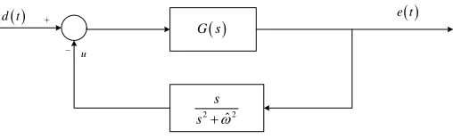
Figure 3.2: Block diagram of continuous system with one internal model
θ(t)= ∠x1ccpq+ jx2ccpq
qωˆp =
d dtθ(t)=
˙
x1ccpqx2ccpq −x1ccpqx˙2ccpq
x21ccpq +x22ccpq
=
qωpx2ccpq+K1ccpqe
x2ccpq−x1ccpq
−qωpx1ccpq+K2ccpqe
x2
1ccpq+ x
2 2ccpq
qωˆp= qωp+
K1ccpqx2ccpq −K2ccpqx1ccpq
x12ccpq +x22ccpq e (3.9)
qω˜p =
K1ccpqx2ccpq−K2ccpqx1ccpq
x2
1ccpq+ x
2 2ccpq
3.2
System with One Internal Model (O
ff
-Line Tuning)
3.2.1
Continuous time
In [55], we know that by designing the closed loop system to be equal to band-pass filter with
notches, we can achieve required stability in our system. The transfer function of a 2nd order
band-pass filter is
Tbp(s)=
B· s2
s4+C
1s3+C2s2+C3s+C4
(3.10)
Coefficients of band-pass filter
C1 C2 C3 C4 B
200.0208 3.8974∗104 2.3690∗105 1.4027∗106 3.2624∗104
Table 3.1: Coefficients of band-pass filter (continuous time)
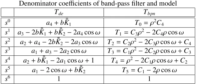
Denominator coefficients of band-pass filter and model
Tde Tbpn
s0 a
4ω2 C4ω2
s1 a3ω2 C3ω2+2εωC4
s2 a4+a2ω2+K1b C2ω2+2εωC3+C4
s3 a
3+a1ω2+K2b C1ω2+2εωC2+C3
s4 a
2+ω2 ω2+C1·2εω+C2
s5 a1 2εω+C1
s6 1 1
Table 3.2: Denominator coefficients of band-pass filter and model (continuous time)
Tn(s)=
s2+ω2
s2+2εωs+ω2 (3.11)
The overall transfer function of Fig. 3.2 is
Tde(s)=
G(s)
1+G(s)·K2s+K1 s2+ω2
(3.12)
where
G(s)= b·s
2
s4+a
1s3+a2s2+a3s+a4
(3.13)
After expanding the denominators ofTdeandG(s), we can get every coefficients of the polynomial as the Table. 3.2 below.
We are designing a fourth order Chebyshev Type I band-pass filter which passes frequencies
between 2π and 60π with 1 dB of ripple in the passband. The coefficients of the denominator of band-pass filter is shown as Table. 3.1.
Coefficients of model
a1 2εω+C1 205.2987
a2 C1·2εω+C2 4.0029∗104
a3
C3ω2+2εωC4
/ω2 2.4753∗105
a4 C4 1.4027∗106
K1
C2ω2+2εωC3+C4−a4−a2ω2
/b 15.7897
K2
C1ω2+2εωC2+C3−a3−a1ω2
/b 5.8666
b B 3.2624∗104
Table 3.3: Coefficients of model (continuous time)
3.3
System with More than One Internal Model (Online
tun-ing)
3.3.1
Continuous time
This section is also written in [32]. Here, a 2nd order band-pass filter is given in Eq. 3.10. And the
notches are expressed as
Tn =
Y s2+(qωˆp)2 s2+2
pqqωˆps+(qωˆp)2
(3.14)
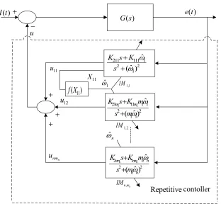
The diagram of the model is shown in Fig. 3.3. The block f (X11) is the adaptation function
shown in Eq. 3.8.
Thus, the desired closed loop has transfer function is
Tbpn =
d1s2
s4+c
1s3+c2s2+c3s+c4
×Y s
2+(qωˆp)2
s2+2
pqqωˆps+(qωˆp)2
(3.15)
The transfer function of the model in Fig. 3.3 is
Tde=
G(s)
1+G(s)Pn
p=1
Pmi
q=1
K2pqs+K1pqqωˆp
s2+(qωˆ
p)2
= b1s2Q(s2+(qωˆp)2)
a(s)Q
(s2+(qωˆp)2)+b
1s2P(K2kls+K1kllωˆk)γkl(s)
text text text text text text ( )
d t e t( )
G s( )
211 111 1
2 2
1
ˆ ˆ
( ) K s K
s 1 1
21 11 1 1
2 2 1 1 ˆ ˆ ( ) m m
K s K m s m 1,1 IM 1,2 IM ,n n m IM u 12 u n nm u . 11 ( ) f X 2 1 2 2 ˆ ˆ ( ) n n
nm nm n n
n n K s K m
s m Repetitive contoller 11 X ˆn 11 u 1 ˆ
Figure 3.3: Block diagram of continuous system with more than one internal model
where
γkl = ni
Y
p=1
mi
Y
q= 1
{p,lifq=k}
(s2+(qωˆp)2) (3.17)
NoteQ
in all equations representsQn p=1
Qmi
q=1and
P
representsPn k=1
Pmk
l=1. The termsγklare the
product of all the terms s2+(qωˆp)2except theq= k, p= lterm.
By matching the numerators,b1can be easily calculated,b1 = d1. Matching the denominators
generates 2nt +4 coupled equations. This generates 2nt+4 unknowns wherent =Pni=1mi. which
is too complex for a computer to solve efficiently. Now, we will show a less computationally intensive algorithm to calculate these unknowns.
setting up 4 equations with 4 unknowns. One characteristic of Tde is that the first term of the
denominator will become zero when s = ±jlωˆk, and the many terms in sum notation will be reduced to only one term. Utilizing this, when s = ±jlωˆk, we can equate the denominators of the transfer function as:
b1s2(K2kls+K1kllωˆk)γkl(s)
= (s4+c1s3+c2s2+c3s+c4)Q Q(s2+2pqqωˆps+(qωˆp)2)
(3.18)
For every pair oflandk, 3.18 generates two equations containing two unknownsK2klandK1kl.
3.3.2
Linear dependence
When the lωk , qωp,for p , k , the gains of internal models can be solved as above. However,
it cannot be solved if lωk = qωp or lωk is pretty close to qωp because the denominator in Tde will be zero. To deal with this situation, we need to drop the redundant internal model. After
calculating the gains, i.e. K1pq, K2pq, the original gains for these two repeated internal models will
beK1pq= K1lq = 0.5K1pqandK2pq = K2lq =0.5K2pq.
3.4
Summary
This chapter shows the basics of this thesis which are done by prior researchers. At the beginning
of this chapter, we showed how the internal models can be used to identify the frequencies.
Mathe-matical derivations are illustrated both in continuous time domain and discrete time domain. Then,
Algorithm Development
4.1
Alternative Model in Discrete Time
With the sample period of T = 1, the previous state space of each internal model I Mpq can be written as the time varying discrete state space model:
Xpq(k+1)= ApqXpq(k)+Bpqe(k)
upq(k)= CpqXpq(k)
(4.1)
where the state isXpq(k)=
x1pq(k) x2pq(k)
T
. AndApq, Bpq andCpqcan be expressed as
Apq =
"
cosqωp −sinqωp sinqωp cosqωp
#
Bpq =
K1ccpqsinqωp
ω −
K2ccpq(1−cosqωp)
ω
K2ccpqsinqωp
qωp +
K1ccpq(1−cosqωp)
qωp
= " ¯ K1pq
¯
K2pq
#
Cpq=
h
0 1 i
(4.2)
The transfer function of this internal model , where we have dropped the time dependencies for
the sack of simplicity, is:
TI M =
K1ccpq−K1ccpqcosqωp+K2ccpqsinqωp
z+K1ccpq−K1ccpqcosqωp−K2ccpqsinqωp
qωp
z2−2zcosqω
p+1
+
- u
G z
d k e k
2 1 2 ˆ
2 cos 1 K z K
z z
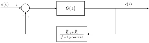
Figure 4.1: Block diagram of discrete system with one internal model
We assign ¯¯Kas in Fig. 4.1 and deduceKbackward as:
¯¯
K1pq =
K1ccpq−K1ccpqcosqωp−K2ccpqsinqωp
qωp
¯¯
K2pq =
K1ccpq−K1ccpqcosqωp+K2ccpqsinqωp
qωp
K1ccpq = (
¯¯
K1pq+K¯¯2pq)qωp
2(1−cosqωp)
K2ccpq = (
¯¯
K2pq−K¯¯1pq)qωp
2 sinqωp
(4.4)
Since it is the discrete time implementation of adaptive model in continuous time, the states
of these two models are same when the input only changes at the sample times. Here, we use the
same adaptation law as previous one:
4ωp=
K1ccp1x2p1−K2ccp1x1p1
x21p1+x22p1 (4.5)
4.2
System with One Internal Model (O
ff
-Line Tuning)
We have shown the off-line tuning in continuous time in Chapter 3. The tuning in discrete time is shown below.
4.2.1
Discrete time
The simple model structure in discrete time is shown in Fig. 4.1.
The transfer function of band-pass filter is
Tbp(z)=
Bz4−2z+1
The notch has the transfer function as
Tn(z) = (
z−ejω)(z−e−jω)
(z−e−εω+jω)∗(z−e−εω−jω)
= z2−2zcosω+1 z2−2zρcosω+ρ2
(4.7)
Here, the small numberρis assigned as
ρ=e−εω
The point wise in time transfer function of the model is
Tde(z)=
G(z)
1+G(z)·
¯¯
K2z+K¯¯1 (z−ejω)(z−e−jω)
(4.8)
where
G(z)= b
z4−2z2+1
z4+a
1z3+a2z2+a3z+a4
(4.9)
So,Tdecan be expanded as
Tde(z)=
bz4−2z2+1·z2−2zcosω+1
z4+a
1z3+a2z2+a3z+a4· z2−2zcosω+1+b· z4−2z2+1·
¯¯
K2z+K¯¯1
(4.10)
After expanding the denominators ofTdeandG(z), we can get every coefficients of the polynomial as the Table. 4.1 below.
Here, we use a 4th-order Chebyshev Type I band-pass filter with a lower passband frequency
of 1· 2π/400 Hz and a higher passband frequency of 30 · 2π/400 Hz. The coefficients of the denominator of band-pass filter is shown as Table. 4.2.
Denominator coefficients of band-pass filter and model
Tde Tbpn
s0 a
4+bK¯¯1 T0 =ρ2C4
s1 a3−2bK¯¯1+bK¯¯2−2a4cosω T1 =C3ρ2−2C4ρcosω
s2 a2+a4−2bK¯¯2−2a3cosω T2 =C2ρ2−2C3ρcosω+C4
s3 a
1+a3−2a2cosω T3 =C1ρ2−2C2ρcosω+C3
s4 a
2+bK¯¯1−2a1cosω+1 T4 =ρ2−2C1ρcosω+C2
s5 a1−2 cosω+bK¯¯2 T5 =C1−2ρcosω
s6 1 1
Table 4.1: Denominator coefficients of band-pass filter and model (discrete time)
Coefficients of band-pass filter
C1 C2 C3 C4 B ρpq
−2.0264 1.4312 −0.7174 0.3153 0.2664 0.9934
Table 4.2: Coefficients of band-pass filter (discrete time)
Coefficients of model
a1 T5+2 cosω−bK¯¯2 −2.0136
a2 T4−bK¯¯1+2a1cosω−1 1.4173
a3 T3−a1+2a2cosω −0.7125
a4 T0−bK¯¯1 0.3116
K1 / −0.0015
K2 / 0.0015
b B 0.2664
Table 4.3: Coefficients of model (discrete time)
Calculation of ¯¯K Tde = b·
z4−2z+1·K¯¯2z+K¯¯1
= zzi·
¯¯
K2zi+K¯¯1
Tbpn
z1 =ejω zz1·K¯¯2·z1+zz1·K¯¯1 −2.8972∗10−6−2.7712∗10−6j
z2 =e−jω zz2·K¯¯2·z2+zz2·K¯¯1 −2.8972∗10−6+2.7712∗10−6j
Table. 4.4 shows a pair of equations with two unknowns, ¯¯K1 and ¯¯K2. This work is the
founda-tion of later secfounda-tions and makes our main algorithm easy to understand.
4.3
System with More than One Internal Model (Online
tun-ing)
4.3.1
Continuous time
In chapter 3 state that the 4 parametersaican be solved by equating the denominators of the transfer
function at any 4 imaginary random values of s. Thiswork is an original contribution of this thesis
and was originally presented in [32]. We have that
Qnt
i=0(s+ri) = s nt +P
risnt−1+Pi
P
j>irirjsnt−2
+· · ·+ sP
i
Q
j,irj+Qri
(4.11)
also,
Qnt
i=1(s
2+2
iωi+ω2i) = s2 nt +P
2iωis2nt−1
+P
ω2
i +
P
i
P
j>i4jωjiωi
s2nt−2
+· · ·+ sP
i2iωiQj,iω2j +
Qω2
i
(4.12)
So,ai(i=1,2,3,4) can be solved by matching the coefficients of the degree 0,1,2nt+2,2nt+3 terms of the denominators ofTdeandTbpn. Setting{ωp}={qωp}and{p}= {pq}, we get
a1 = c1+P2pωp
a2 = P
nt
p=1
P
q>i4qωqpωp+c1P
nt
p=12pωp+c2
a3 = c3+c4P
nt
p=12p/ωp
a4 = c4
(4.13)
4.3.2
Discrete time
The signal we use in discrete time is of the following form:
d(k)= n X =1 mp X =1
+ -+ + + Repetitive Controller (z) G
( )11,
f x e
11 IM 21 IM pq IM 21 u d e u 11 x 11 u pq u
( 1)( 1)
221 121 ˆ ˆ 2 2
K z K z e z e−
+
− −
( 2 )( 1 )
ˆq ˆq pq pq
p p
K z K z e z e−
+ − − 1 a K z z− ˆ g h , a b
( 1)( 1)
211 111 ˆ ˆ
K z K z e z e−
+
− −
1 ,ij 2ij
K K
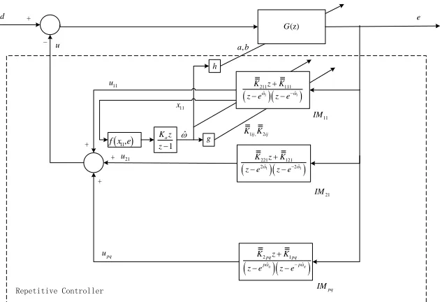
Figure 4.2: Structure of signal identification based on the internal model
where the phase is given by
φpq(k)= k
X
i=1
qωp(k)+φpq(0) (4.15) Here,nis noise and the signals are the sum of n time-varying sinusoidal waves withmp
harmonics each. It is assumed that the frequencies and amplitudes vary slowly in time. Apq,ωp
andφpqare unknown and uncertain magnitude, frequency, and relative phases respectively.
Fig. 4.2 shows structure of the instantaneous Fourier decomposition algorithm.G(z) is a tuning
function paralleled with internal models. Functions of f, gandhis shown in Eq. 4.5, Eq. 4.4 and
Eq. 4.25 to 4.28 respectively. Each transfer function I Mpq represents a corresponding sinusoidal
with the frequency ofqωp. The transfer function of each internal model has poles at e±qωˆp. Note
that thenfundamental frequencies are calculated only using the states of the fundamental harmonic
model. This is based on the assumption that the fundamental typically has more energy than the
harmonics. This is not necessary, any model can be used in the case where the fundamental is
absent. Alternative choices include estimating the frequency based on the model with the greatest
0 0.1 0.2 0.3 0.4 0.5 0.6 0.7 0.8 0.9 1 Normalized Frequency ( rad/sample)
-200 -100 0 100 200
Phase (degrees)
0 0.1 0.2 0.3 0.4 0.5 0.6 0.7 0.8 0.9 1 Normalized Frequency ( rad/sample)
-150 -100 -50 0
Magnitude (dB)
Figure 4.3: Bode diagram of band-pass filter
To identify all frequencies in the signal in equation 4.14, a suitable gain needs to be chosen to so
that this remains a stable feedback loop. This situation has already been successfully implemented
to reject unknown periodic disturbances in magnetic hard disk drives[36]. However, this brings
a lot of restrictions to our algorithm. As we discussed in Chapter 2, there is no control over the
dynamic system in our case, thus, we need to tune the gain adaptively.
4.3.3
Band-pass filter
Fig. 4.3 and Fig. 4.4 show the theoretical Bode plot of desired band-pass filter and band-pass filter
with ten notches respectively. Here, we use a 4th-order Chebyshev Type I band-pass filter with a
lower passband frequency of 1·2π/400 Hz and a higher passband frequency of 30·2π/400 Hz.
4.3.4
Parameter calculation
0 0.1 0.2 0.3 0.4 0.5 0.6 0.7 0.8 0.9 1 Normalized Frequency ( rad/sample)
-1000 0 1000 2000 3000
Phase (degrees)
0 0.1 0.2 0.3 0.4 0.5 0.6 0.7 0.8 0.9 1 Normalized Frequency ( rad/sample)
-300 -200 -100 0 100
Magnitude (dB)
Figure 4.4: Bode diagram of band-pass filter with notches
Tbpn(z) =
B1(z4−2z+1) z4+C
1z3+C2z2+C3z+C4 ∗
Q (z−ejqωp)(z−e
−jqωp)
(z−ρpqejqωp)∗(z−ρpqe−jqωp)
= B1(z4−2z+1) z4+C
1z3+C2z2+C3z+C4 ∗
Q z2−2zcosqωp+1
z2−2zρ
pqcosqωp+ρ2pq
(4.16)
Here, the small numberρpqis calculated by
ρpq= e
−εpqqωp
Here,εpq are small real numbers, andqωpare the notches frequency. The presence of zeros
(roots) atejqωp in the numerator is a fundamental consequence of the internal model principle.
Therefore, the algorithm has a better ability to improve noise rejection. By transferring the
system from the s-domain, the point wise in time transfer function fromdtoeinz-domain is
Tde(z)=
G(z)
1+G(z)Pn p=1
Pmp
q=1
¯¯
K2pqz+K¯¯1pq
(z−ejqωp)(z−e−jqωp)
(4.17)
G(z)= b1
z4−2z+1
z4+a
1z3+a2z2+a3z+a4
= b(z)
a(z) (4.18)
The numerator ofTdeis
Tdenum(z)=b1
z4−2z+1 Y z2−2zcosqωp+1
(4.19)
and the denominator ofTdeis
Tdeden(z) = a(z)
Q
z2−2zcosqωp+1
+b1
z4−2z+1Pn p=1
Pmp
q=1
h¯¯
K2pqz+K¯¯1pq
Υpq(z)i (4.20)
where
Υpq(z)= n
Y
k=1
mp
Y
l=1
l, p i f p=k
z2−2zcoslωk +1
(4.21)
Apparently, by matching the numerator ofTdeandTbpn, we can get that
b1 = B1 (4.22)
As what we showed in Chapter 3, if we look at the equations carefully, we can find that when
z=e±jqωp, we have
b1
z4−2z+1 n
X
p=1
mp
X
q=1
¯¯
K2pqz+K¯¯1pq
Υkl(z)=C(z)∗Y z2−2zρpqcosqωp+ρ2pq
(4.23)
Thus, every substitution ofe±jqωp will generate 2 equations with two unknowns of ¯¯K
2pq and ¯¯K1pq.