NEAR-FIELD — FAR-FIELD TRANSFORMATION TECHNIQUE WITH HELICOIDAL SCANNING FOR ELONGATED ANTENNAS
F. D’Agostino, F. Ferrara, C. Gennarelli, R. Guerriero and M. Migliozzi
Dipartimento di Ingegneria dell’Informazione ed Ingegneria Elettrica University of Salerno, via Ponte Don Melillo
Fisciano 84084, Salerno, Italy
Abstract—A fast and accurate near-field — far-field transformation
technique with helicoidal scanning is proposed in this paper. It is tailored for elongated antennas, since a prolate ellipsoid instead of a sphere is considered as surface enclosing the antenna under test. Such an ellipsoidal modelling allows one to consider measurement cylinders with a diameter smaller than the antenna height, thus reducing the error related to the truncation of the scanning surface. Moreover, it is quite general, containing the spherical modelling as particular case, and allows a significant reduction of the number of the required near-field data when dealing with elongated antennas. Numerical tests are reported for demonstrating the accuracy of the far-field reconstruction process and its stability with respect to random errors affecting the data.
1. INTRODUCTION
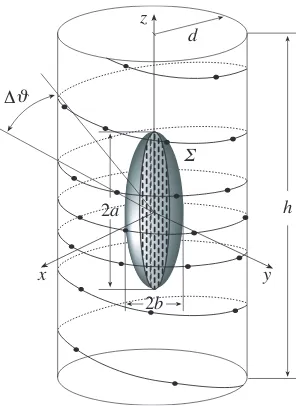
y x
d ∆
2a
2b
Σ z
h ϑ
Figure 1. Helicoidal scanning.
However, the use of the spherical AUT modelling prevents the possibility of considering measurement cylinders (planes) with a radius (distance) smaller than one half the source maximum size. This drawback occurs in the helicoidal and in the planar spiral scannings when considering elongated and quasi-planar antennas, respectively. Obviously, this reflects in an increase of the error related to the truncation of the scanning surface. In fact, for a given size of the scan zone, such an error raises on increasing the distance. Moreover, the volumetric redundancy of the spherical modelling gives rise to an increase in the number of the NF data, when the AUT geometry departs from the spherical one.
The aim of this paper is to develop an efficient NF-FF transformation technique with helicoidal scanning tailored for elongated antennas, which allows to overcome the abovementioned drawbacks. To this end, the AUT is considered as enclosed in a prolate spheroid (Fig. 1), a shape particularly suitable to deal with such a kind of antennas, but which remains quite general and contains the spherical modelling as particular case.
2. THE SPHERICAL MODELLING OF THE ANTENNA
Let us consider a non directive probe which scans a helix with constant angular step lying on a cylinder of radius d surrounding the AUT (see Fig. 1) and adopt the spherical coordinate system (r, ϑ, ϕ) for denoting the observation point P in the NF region. Since the voltage
V measured by this kind of probe has the same effective spatial bandwidth of the field, the theoretical results on the nonredundant representation of EM fields [9] can be applied to such a voltage. Accordingly, if the AUT is enclosed in a sphere of radius a (AUT ball) and the helix is described by a proper analytical parameterization
r=r(ξ), the probe “reduced voltage”
˜
V(ξ) =V(ξ)ejγ(ξ) (1)
can be closely approximated by a spatially bandlimited function,γ(ξ) being a phase function to be determined. The related bandlimitation error becomes negligible as the bandwidth exceeds a critical value
Wξ [9], so that it can be effectively controlled by choosing a bandwidth equal to χWξ, wherein the excess bandwidth factor χ is slightly
greater than unity for an electrically large AUT.
sample spacing needed to interpolate the voltage along a cylinder generatrix.
The parametric equations of the helix, when imposing its passage through a fixed point Q0 of the generatrix at ϕ = 0, are: x = dcos(φ−φi), y = dsin(φ−φi), z = dcotθ, where φ is the angular parameter describing the helix,φi is the value ofφatQ0, andθ=kφ.
The parameter k is such that the angular step, determined by the consecutive intersections Q(φ) and Q(φ+ 2π) with a generatrix, is ∆θ= 2πk. It is worth noting that the helix can be obtained by radially projecting on the measurement cylinder the spiral wrapping the AUT ball with the same angular step.
As shown in [7], a nonredundant sampling representation of the voltage on the helix can be obtained by using the following expressions for the optimal phase function and parameterization:
γ = β
r
0
1−a2/r2dr =βr2−a2−βacos−1a r
(2)
ξ = βa
Wξ
φ
0
k2+ sin2kφdφ (3)
whereβ is the wavenumber.
Since the elevation step of the helix must be equal to the sample spacing required for the interpolation along a generatrix, then, according to [9], ∆θ = ∆ϑ= 2π/(2N+ 1), withN = Int(χN) + 1 and N = Int(χβa) + 1, χ > 1 being an oversampling factor. As a consequence, k= 1/(2N+ 1).
According to (3),ξis proportional to the curvilinear abscissa along the spiral wrapping the sphere modelling the source. Since such a spiral is a closed curve, it is convenient to choose the bandwidthWξsuch that
ξ covers a 2π range when the whole curve on the sphere is described. As a consequence,
Wξ= βa
π
(2N+1)π
0
k2+ sin2kφdφ (4)
According to these results, the optimal sampling interpolation (OSI) formula of central type to reconstruct the voltage at any point Q of the helix is [7, 9]:
˜
V(ξ) =
m0+p
m=m0−p+1
˜
wherem0 = Int[(ξ−ξ(φi))/∆ξ] is the index of the sample nearest (on
the left) to the output point, 2p is the number of retained samples ˜
V(ξm), and
ξm=ξ(φi) +m∆ξ=ξ(φi) + 2πm/
2M+ 1 (6)
withM= Int(χM) + 1 andM = Int(χWξ) + 1.Moreover,
DM(ξ) =
sin ((2M+ 1)ξ/2) (2M+ 1) sin(ξ/2);
ΩM(ξ) = TM
−1 + 2cos(ξ/2)/cosξ/¯ 2 2
TM[−1 + 2/cos2
¯
ξ/2 ]
(7)
are the Dirichlet and Tschebyscheff Sampling functions, whereinTM(ξ)
is the Tschebyscheff polynomial of degreeM =M−Mand ¯ξ =p∆ξ. The OSI formula (5) can be used to evaluate the “intermediate samples”, namely, the voltage values at the intersection points between the helix and the generatrix passing through P. Once these samples have been evaluated, the voltage at P can be reconstructed via the following OSI expansion:
˜
V(ϑ, ϕ) =
n0+q
n=n0−q+1
˜
V (ϑn) ΩN(ϑ−ϑn)DN(ϑ−ϑn) (8)
where N =N−N,n0 = Int[(ϑ−ϑ0)/∆ϑ], 2q is the number of the
retained intermediate samples ˜V(ϑn), and
ϑn=ϑn(ϕ) =ϑ(φi) +kϕ+n∆ϑ=ϑ0+n∆ϑ (9)
The described two-dimensional OSI algorithm can be properly applied to recover the NF data required by the NF–FF transformation technique [10].
3. THE PROLATE ELLIPSOIDAL MODELLING OF THE ANTENNA
redundancy of the spherical modelling gives rise to a useless increase in the number of NF data, when the AUT geometry departs from the spherical one. To overcome these drawbacks, the previously described sampling representation will be properly extended in this Section to the case of elongated antennas.
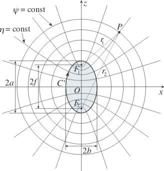
C'
F2 F2
= const
ψ
= const
η
2b
z
2a
P
x
O
2f
r1
r2 F1
Figure 2. Ellipsoidal source modelling.
An effective modelling for this kind of antennas is obtained by considering them as enclosed in the smallest prolate ellipsoid having major and minor semi-axes equal to a and b (see Fig. 2). In such a case, by adoptingWη =β#/2π (# being the length of the intersection
curveC between the meridian plane throughP and the ellipsoid), the optimal expressions for the phase functionψand the parameterization
η to be used for describing a cylinder generatrix become [9]:
ψ = βa
v
(v2−1)
(v2−ε2)−E
cos−1
(1−ε2)
(v2−ε2)|ε 2
(10)
η = (π/2)1 +Esin−1u|ε2 /Eπ/2|ε2 (11)
whereu= (r1−r2)/2f andv= (r1+r2)/2aare the elliptic coordinates, r1,2 being the distances fromP to the foci and 2f the focal distance of C. Moreover,ε=f /ais the eccentricity ofC, andE(·|·) denotes the elliptic integral of second kind. It is worth noting that in any meridian plane the curves ψ= const and η = const are ellipses and hyperbolas confocal to C (Fig. 2), instead of circumferences and radial lines.
the scanning cylinder. The elevation step of such a spiral is equal to the sample spacing ∆η needed for the voltage interpolation along a generatrix. The projection is now obtained by means of the hyperbolas atη = const, that in the case of spheroidal source modelling take the role of the radial lines of the spherical one. Accordingly, the parametric equations of the helix become:
x=dcos (φ−φ
i) y=dsin (φ−φi)
z=dcot[θ(η)]
(12)
whereinη=kφ=φ/(2N+ 1).
A quite analogous reasoning allows one to determine the phase function and the parameterization to be used for obtaining a nonredundant sampling representation along the helix. In particular, by generalizing relations (2) and (3), the phase function γ coincides with ψ defined in (10) and the parameter ξ is β/Wξ times the
curvilinear abscissa of the projecting point that lies on the spiral wrapping the ellipsoid. Moreover, according to (4), Wξ is chosen to
be equal to β/π times the length of the spiral wrapping the ellipsoid from pole to pole. As a conclusion, the spiral, γ and ξ are such that they coincide with those relevant to the spherical modelling when the prolate ellipsoid approaches to a sphere.
It is worthy to note that the OSI formula (5) can be still used to reconstruct the reduced voltage at any point on the helix and, as a consequence, can be applied to recover the intermediate samples, whereas the NF data required to carry out the NF-FF transformation [10] can be reconstructed by means of the following OSI expansion:
˜
V(η(ϑ), ϕ) =
n0+q
n=n0−q+1
˜
V (ηn) ΩN(η−ηn)DN(η−ηn) (13)
whereinN =N−N,N = Int(χWη) + 1,n0= Int[(η−η0)/∆η], 2q
is the number of the retained intermediate samples ˜V(ηn), and
ηn=ηn(ϕ) =η(φi) +kϕ+n∆η=η0+n∆η (14)
4. NF-FF TRANSFORMATION
coefficients aν and bν of the cylindrical wave expansion of the field
radiated by the AUT are related to: i) the two-dimensional Fourier transforms Iν and Iν of the output voltage of the probe for two
independent sets of measurements (the probe is rotated 90◦ about its longitudinal axis in the second set); ii) the coefficients cm, dm and
cm, dm of the cylindrical wave expansion of the field radiated by the probe and the rotated probe, respectively, when used as transmitting antennas. The key relations are:
aν(α) = β
2
Λ2∆ ν(α)
Iν(α)
∞
m=−∞
dm(−α)Hν(2)+m(Λd)
−Iν(α)
∞
m=−∞
dm(−α)Hν(2)+m(Λd)
(15)
bν(α) = β
2
Λ2∆ ν(α)
Iν(α)
∞
m=−∞
cm(−α)Hν(2)+m(Λd)
−Iν(α) ∞
m=−∞
cm(−α)Hν(2)+m(Λd)
(16)
Iν(α) =
∞ −∞ π −π
V(ϕ, z)e−jνϕejαzdϕdz;
Iν(α) =
∞ −∞ π −π
V(ϕ, z)e−jνϕejαzdϕdz
(17)
∆ν(α) = ∞
m=−∞
cm(−α)Hν(2)+m(Λd)
∞
m=−∞
dm(−α)Hν(2)+m(Λd)
− ∞
m=−∞
cm(−α)Hν(2)+m(Λd)
∞
m=−∞
dm(−α)Hν(2)+m(Λd) (18)
where Λ = β2−α2, H(2)
ν (·) is the Hankel function of second kind
and orderν, andV,V represent the output voltage of the probe and the rotated probe at the point (d, ϕ, z).
(R,Θ,Φ) can be evaluated by:
EΘ(R,Θ,Φ) = −j2β e−jβR
R sin Θ ∞
ν=−∞
jνbν(βcos Θ)ejνΦ (19)
EΦ(R,Θ,Φ) = −2β e−jβR
R sin Θ ∞
ν=−∞
jνaν(βcos Θ)ejνΦ (20)
5. NUMERICAL TESTS
Some numerical tests assessing the effectiveness of the developed technique are reported in the following. The first simulation refers to a uniform planar array (Fig. 1) of elementary Huygens sources polarized along the z axis. Its elements cover an elliptical zone in the plane
y = 0, with major and minor semi-axes equal to 30λand 6λ, and are spaced by 0.4λalong x and 0.6λalongz,λbeing the wavelength. An open-ended WR-90rectangular waveguide, operating at the frequency of 10GHz, is chosen as probe. The NF data are collected on a helix wrapping a cylinder with radiusd= 12λand heighth= 180λ.
-60 -50 -40 -30 -20 -10 0
-90 -75 -60 -45 -30 -15 0 15 30 45 60 7 90
Relative output voltage amplitude (dB)
q =p = 6
χ = 1.20
χ' = 1.20
z (wavelengths) 5
Figure 3. Amplitude of V
on the generatrix at ϕ = 90◦. Solid line: exact. Crosses: interpolated.
-180 -135 -90 -45 0 45 90 135 180
0 10 20 30 40 50 60 70 8 90
Output voltage phase (degrees)
q =p = 6
χ = 1.20
χ' = 1.20
z (wavelengths) 0
Figure 4. Phase of V on the
generatrix atϕ= 90◦. Solid line: exact. Crosses: interpolated.
with those directly evaluated on a close grid in the central zone of the cylinder, so that the existence of the guard samples is assured. As expected, the errors decrease up to very low values on increasing the oversampling factor and/or the number of the retained samples. The algorithm stability has been investigated by adding random errors to the exact samples. These errors simulate a background noise, bounded to ∆ain amplitude and with arbitrary phase, and uncertainties on the data of ±∆ar in amplitude and ±∆σ in phase. As shown in Fig. 7, the interpolation algorithm works well also when dealing with error affected data. The reconstructions of the antenna FF pattern in the principal planes are shown in Figs. 8 and 9. As can be seen, the exact and recovered fields are practically indistinguishable, thus assessing
χ' = 1.20
-90 -80 -70 -60 -50 -40 -30 -20
2 3 4 5 6 7 8 9 10 11 12 13
Normalized maximum error (dB)
p = q
χ = 1.10
χ = 1.15
χ = 1.20
χ = 1.25
Figure 5. Normalized maximum
reconstruction error.
χ' = 1.20
-110 -100 -90 -80 -70 -60 -50 -40 -30
2 3 4 5 6 7 8 9 10 11 12 13
Normalized mean-square error (dB)
p = q
χ = 1.10
χ = 1.15
χ = 1.20
χ = 1.25
Figure 6. Normalized
mean-square reconstruction error.
-60 -50 -40 -30 -20 -10 0
-90 -75 -60 -45 -30 -15 0 15 30 45 60 75 90
Relative output voltage amplitude (dB)
z (wavelengths)
q =p = 6
χ = 1.20
χ' = 1.20
∆a = -50 dB
∆a = 0.5 dB
∆σ = 5o r
Figure 7. Amplitude of V
on the generatrix at ϕ = 90◦. Solid line: exact. Crosses: interpolated from error affected data. -90 -80 -70 -60 -50 -40 -30 -20 -10 0
20 30 40 50 60 70 80 90
Relative field amplitude (dB)
q =p = 9
χ = 1.20
χ' = 1.20
Θ (degrees)
Figure 8. E-plane pattern.
the effectiveness of the developed NF–FF transformation technique. Note that the number of the samples employed for reconstructing the NF data over the considered cylinder is 15153 (guard samples included), significantly less than that (46080) required by the approach in [11].
As already stated, the use of the spherical AUT modelling prevents the possibility of considering measurement cylinders with a radius smaller than one half the antenna maximum size, thus giving rise to an increase of the truncation error for a given size of the scanning zone. In order to highlight this drawback, another reconstruction of the E-plane pattern, obtained by employing the spherical modelling, is shown in Fig. 10. In such a case, the NF data have been collected on a helix that covers a cylinder having the same height but radius of 36 λ. As can be clearly seen, the reconstruction is less accurate in the far out side lobe region.
-80 -70 -60 -50 -40 -30 -20 -10 0
90 120 150 180 210 240 270
Relative field amplitude (dB)
q =p = 9
χ = 1.20
χ' = 1.20
Φ (degrees)
Figure 9. H-plane pattern.
Solid line: exact. Crosses: recon-structed from NF measurements.
-90 -80 -70 -60 -50 -40 -30 -20 -10 0
20 30 40 50 60 70 80 90
Relative field amplitude (dB)
q =p = 9
χ = 1.20
χ' = 1.20
Θ (degrees)
Figure 10. E-plane pattern.
Solid line: exact. Crosses: recon-structed from NF measurements when using the spherical mod-elling.
-70 -60 -50 -40 -30 -20 -10 0
20 30 40 50 60 70 80 90
Relative field amplitude (dB)
q =p = 9
χ = 1.20
χ' = 1.20
Θ (degrees)
Figure 11. E-plane pattern of a Tschebyscheff array. Solid line:
exact. Crosses: reconstructed from NF measurements.
6. CONCLUSIONS
An innovative NF-FF transformation with helicoidal scanning has been developed in this paper by using an ellipsoidal modelling of the source, instead of the previously adopted spherical one. Such a modelling, tailored for elongated antennas, allows one to consider measurement cylinders with a diameter smaller than the antenna height, thus reducing the error related to the truncation of the scanning surface. Moreover, it contains the spherical modelling as particular case and lowers significantly the number of required data when dealing with elongated antennas. The reported numerical examples have demonstrated the accuracy of the technique and its stability with respect to random errors affecting the NF data.
REFERENCES
1. Yaccarino, R. G., L. I. Williams, and Y. Rahmat-Samii, “Linear spiral sampling for the bipolar planar antenna measurement technique,”IEEE Trans. Antennas Propagat., Vol. 44, 1049–1051, July 1996.
2. Bucci, O. M., C. Gennarelli, G. Riccio, and C. Savarese, “Probe compensated NF-FF transformation with helicoidal scanning,”
Journal of Electromagnetic Waves and Applications, Vol. 14, 531– 549, 2000.
3. Bucci, O. M., C. Gennarelli, G. Riccio, and C. Savarese, “Nonredundant NF-FF transformation with helicoidal scanning,”
Journal of Electromagnetic Waves and Applications, Vol. 15,
4. Bucci, O. M., F. D’Agostino, C. Gennarelli, G. Riccio, and C. Savarese, “Probe compensated FF reconstruction by NF planar spiral scanning,” IEE Proc. Microw., Ant. Prop., Vol. 149, 119– 123, April 2002.
5. Bucci, O. M., F. D’Agostino, C. Gennarelli, G. Riccio, and C. Savarese, “NF-FF transformation with spherical spiral scanning,”IEEE Antennas Wireless Propagat. Lett., Vol. 2, 263– 266, 2003.
6. D’Agostino, F., F. Ferrara, C. Gennarelli, G. Riccio, and C. Savarese, “Directivity computation by spherical spiral scanning in NF region,” Journal of Electromagnetic Waves and Applications, Vol. 19, 1343–1358, 2005.
7. D’Agostino, F., C. Gennarelli, G. Riccio, and C. Savarese, “Theoretical foundations of near-field — far-field transformations with spiral scannings,” Progress In Electromagnetics Research, PIER 61, 193–214, 2006.
8. Gennarelli, C., G. Riccio, F. D’Agostino, and F. Ferrara,
Near-field — Far-Near-field Transformation Techniques, Vol. 1, CUES,
Salerno, Italy, 2004.
9. Bucci, O. M., C. Gennarelli, and C. Savarese, “Representation of electromagnetic fields over arbitrary surfaces by a finite and nonredundant number of samples,” IEEE Trans. Antennas Propagat., Vol. 46, 351–359, March 1998.
10. Leach, W. M., Jr. and D. T. Paris, “Probe compensated NF measurements on a cylinder,” IEEE Trans. Antennas Propagat., Vol. 21, 435–445, July 1973.