Scholarship@Western
Scholarship@Western
Electronic Thesis and Dissertation Repository
7-23-2019 9:00 AM
Empirical Analysis of Urban Sprawl in Canadian Census
Empirical Analysis of Urban Sprawl in Canadian Census
Metropolitan Areas using Satellite Imagery, 1986-2016
Metropolitan Areas using Satellite Imagery, 1986-2016
Xiaoxuan Sun
The University of Western Ontario
Supervisor Wang, Jinfei
The University of Western Ontario Co-Supervisor Mok, Diana
The University of Western Ontario Graduate Program in Geography
A thesis submitted in partial fulfillment of the requirements for the degree in Master of Science © Xiaoxuan Sun 2019
Follow this and additional works at: https://ir.lib.uwo.ca/etd
Part of the Remote Sensing Commons
Recommended Citation Recommended Citation
Sun, Xiaoxuan, "Empirical Analysis of Urban Sprawl in Canadian Census Metropolitan Areas using Satellite Imagery, 1986-2016" (2019). Electronic Thesis and Dissertation Repository. 6394.
https://ir.lib.uwo.ca/etd/6394
This Dissertation/Thesis is brought to you for free and open access by Scholarship@Western. It has been accepted for inclusion in Electronic Thesis and Dissertation Repository by an authorized administrator of
i
Many Canadian cities have experienced rapid sprawl over the last 30 years. This dissertation presents two studies that empirically examine the causes of urban sprawl, merging census socioeconomics data and satellite imageries of 11 major Census Metropolitan Areas (CMAs). The monocentric city model and the Tiebout model are the main traditional theories
explaining urban boundary changes and residential mobility. The first study focuses on a cross-sectional comparison among the 11 CMAs in 2016. The second study zooms into the Toronto CMA and examine the longitudinal changes in its urban coverage at its fringes. The land cover/use changes are detected within the Toronto CMA from 1986 to 2016. In both studies, the role of price risk is inserted in understanding the timing of urban development. In doing so, both studies aim to contribute to the literature by broadening the traditional theories to include the role of risk as it influences urban development.
Keywords
ii
Summary for Lay Audience
Urban sprawl is one of the most important issues facing most cities around the world. Many Canadian cities have experienced rapid sprawl over the last 30 years. This dissertation presents two studies that empirically examine the causes of urban sprawl, merging census socioeconomics data and satellite imageries of 11 major Census Metropolitan Areas (CMAs) in 1986, 2006 and 2016. Two branches of traditional theories of urban sprawl, the
monocentric city model and the Tiebout model, are used to explain urban boundary changes. The first empirical study focuses on a cross-sectional comparison among the 11 CMAs and attempts to study the role of price risk in influencing the extent of urban coverage expansion outside of the cities covered by the CMA boundaries. The second study focuses on the largest CMA in Canada, Toronto, and examine the longitudinal changes in its urban coverage at its fringes. The land cover/use changes are detected within the Toronto CMA for 1986-2006 and 2006-2016. The 1986, 2006 and 2016 satellite imageries are matched with residents’
iii
Co-Authorship Statement
I am responsible for nearly all data collection and experiments and conducted all statistical analyses and writing of the manuscript. Dr. Jinfei Wang and Dr. Diana Mok assisted with study design and improved the manuscript. In Chapter 3, Diana helped record sales data from the TREB. Matthew J. Roffey collected Landsat 5 satellite data of 1986 and 2005 and
iv
Acknowledgments
I would like to first thank my supervisors, Dr. Jinfei Wang and Dr. Diana Mok, for their guidance and support throughout my two-year journey as a master’s student. They have been available to communicate whenever I needed assistance. Jinfei has provided many comments regarding my work and words of encouragement. Diana has taught me a lot about economics and has inspired me throughout my studies. I will treasure many memories with them
forever. I am grateful to have had the opportunities to present my studies in Washington and Winnipeg at AAG and CAG, respectively.
I would also like to thank the members of our GITA Lab and the Department of Geography administration team. I have had a wonderful time working with you.
v
Table of Contents
Abstract ... i
Summary for Lay Audience ... ii
Co-Authorship Statement... iii
Acknowledgments... iv
Table of Contents ... v
List of Tables ... viii
List of Figures ... x
List of Appendices ... xii
List of Abbreviations ... xiii
Chapter 1 ... 1
1 Introduction ... 1
1.1 Research contents... 1
1.2 Research objectives ... 4
1.3 Study area and data ... 5
1.4 Thesis organization ... 9
1.5 References ... 9
2 Testing Theories of Urban Sprawl Using Sentinel-2 Imagery: A Cross-sectional Comparison among 11 Canadian Census Metropolitan Areas ... 12
2.1 Introduction ... 12
2.1.1 Background ... 12
2.1.2 Previous studies and theories ... 15
2.2 Data and variables ... 17
2.2.1 Study Area ... 17
2.2.2 Data ... 17
vi
2.3 Methods and Empirical Strategy ... 26
2.3.1 Data Pre-processing ... 26
2.3.2 Image Classification... 27
2.3.3 Empirical Strategy ... 29
2.4 Results and Discussion ... 31
2.4.1 Land Cover/Use Estimates ... 31
2.4.2 Statistical Analysis ... 33
2.5 Conclusions ... 35
2.6 References ... 36
3 Analysis of Urban Sprawl in the Toronto Census Metropolitan Area Using Panel Data from 1986 to 2016 ... 39
3.1 Introduction ... 39
3.1.1 Background ... 39
3.1.2 Previous studies and theories ... 41
3.2 Data and variables ... 46
3.2.1 Study area... 46
3.2.2 Data ... 47
3.2.3 Variables ... 51
3.3 Methods... 53
3.3.1 Data pre-processing ... 53
3.3.2 Image classification and accuracy assessment ... 54
3.3.3 Post-classification processing ... 55
3.3.4 Change detection ... 55
3.3.5 Data interpolation... 56
3.3.6 Statistical analysis using the difference-in-difference model ... 58
vii
3.4.1 Accuracy assessment ... 59
3.4.2 Change detection analysis ... 60
3.4.3 Statistical analysis ... 65
3.5 Conclusions ... 67
3.6 References ... 68
4 Conclusions ... 72
4.1 Summary and conclusions ... 72
4.2 Contributions... 73
4.3 Limitations ... 73
4.4 Possible future research ... 74
Appendices ... 75
viii
List of Tables
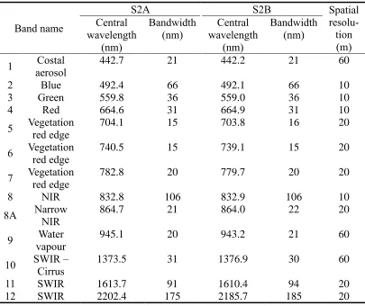
Table 2. 1 Details of the Sentinel-2 spectral bands ... 18
Table 2. 2 Sentinel-2 data acquisition dates (year=2016) ... 19
Table 2. 3 Census data definition ... 20
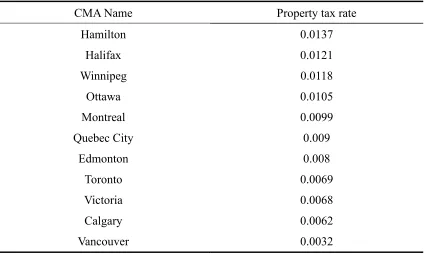
Table 2. 4 Mill rate for the 11 Census Metropolitan Areas in 2016 ... 21
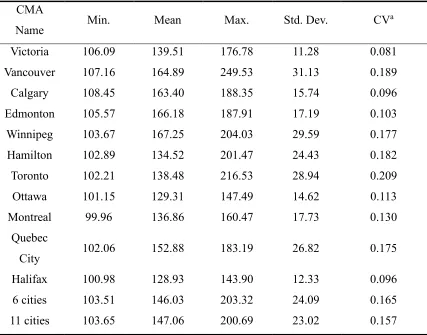
Table 2. 5 Summary statistics of House Price Indices ... 23
Table 2. 6 Summary statistics of the dependent variable (built-up area in the Dissemination Area) for each Census Metropolitan Area ... 24
Table 2. 7 Statistical summaries of the independent variables ... 25
Table 2. 8 Land cover/use classification scheme ... 28
Table 2. 9 Accuracy assessment ... 32
Table 2. 10 OLS estimation results (n=1104) ... 34
Table 3. 1 The implement of the DID model. ... 45
Table 3. 2 Comparison of the characteristics of the sensors between satellites Landsat 5 and Sentinel-2 ... 48
Table 3. 3 Census data definition ... 49
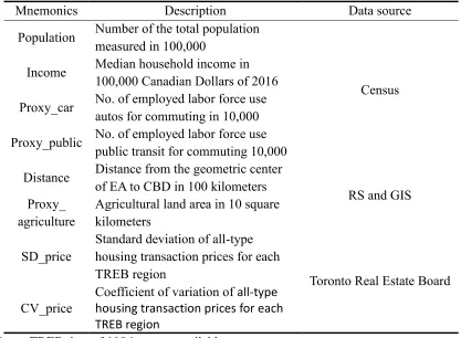
Table 3. 4 Descriptions and sources of the independent variables ... 52
Table 3. 5 Summary statistics of socioeconomic variables among Enumeration Areas (n=6726) ... 52
Table 3. 6 Summary of classification accuracies for 1986, 2005, and 2016 ... 60
ix
Table 3. 8 DID estimation results using distance as the proxy for commuting costs (n=6,726) ... 65
x
List of Figures
Figure 1. 1 Study area ... 7
Figure 2. 1 House Price Indices of the 11 Canadian Census Metropolitan Areas from January 2006 to December 2016 ... 22
Figure 2. 2 Conceptual diagram of the empirical model ... 29
Figure 2. 3 (a) (b) (c) Land cover/use patterns for the 11 Census Metropolitan Areas using zonal statistics ... 32
Figure 3. 1 Study area ... 46
Figure 3. 2 False-color Sentinel-2 satellite imagery of the Toronto Census Metropolitan Area on September 24, 2016 ... 48
Figure 3. 3 Geographic hierarchy for census dissemination ... 50
Figure 3. 4 Flowchart of methods used in this study ... 53
Figure 3. 5 Census units’ boundary changes in the Toronto Census Metropolitan Area 1986, 2006, and 2016 ... 57
Figure 3. 6 Urban area within the Toronto CMA from 1986 to 2016 ... 61
Figure 3. 7 Change detection results (a) 1986-2006; (b) 2006-2016, and (c)1986-2016 ... 62
Figure 3. 8 Change detection of the predominant class in the Enumeration Area (a) 1986-2006; (b) 2006-2016, and (c)1986-2016 ... 64
Figure B. 1 Greenbelt Designation for the Greater Toronto Area ... 77
Figure C. 1 Toronto CMA false-color image map ... 78
Figure C. 2 Montreal CMA false-color image map ... 79
xi
Figure C. 4 Calgary CMA false-color image map ... 81
Figure C. 5 Ottawa-Gatineau CMA false-color image map ... 82
Figure C. 6 Edmonton CMA false-color image map ... 83
Figure C. 7 Quebec CMA false-color image map ... 84
Figure C. 8 Winnipeg CMA false-color image map ... 85
Figure C. 9 Hamilton CMA false-color image map ... 86
Figure C. 10 Halifax CMA false-color image map ... 87
xii
List of Appendices
Appendix A Peripheral municipalities of Census Metropolitan Areas ... 75
Appendix B Greenbelt area ... 76
Appendix C Sentinel-2 imageries for the 11 Census Metropolitan Areas ... 78
xiii
List of Abbreviations
CA — Census Agglomeration
CBD — Central Business District
CMA — Census Metropolitan Area
CPI — Consumer Price Index
CT — Census Tract
CV — Coefficient of Variance
DA — Dissemination Area
DB — Dissemination Block
DID — Difference-In-Difference
EA — Enumeration Area
ESA — European Space Agency
GB — Greenbelt Area
GIS — Geographic Information System
HPI — House Price Index
LTDB — Longitudinal Tract Database
MSI — Multi-spectral Instrument
NPV — Net Present Value
RS — Remote Sensing
xiv
SI — Sprawl Index
TREB — Toronto Real Estate Board
Chapter 1
1
Introduction
1.1
Research contents
Urban sprawl, a term often used to refer to leapfrog developments in the urban fringe, is commonly considered detrimental to activities of both the economy and the environment. Its negative impacts include, but are not limited to, higher levels of pollution, loss of agricultural land and green space, and increased commuting time (McGibany, 2004). Thus, sprawl has become a national debate for both the public and the government. Sprawl refers to the natural expansion of metropolitan areas as population grows
(Brueckner & Fansler, 1983). Strong sentiment against sprawl has developed over the last decade in North American cities, particularly among Canadian cities—for example, among all 35 Census Metropolitan Areas (CMAs) in Canada, populations in central municipalities increased by 5.8%, compared to a 6.9% jump in the peripheral municipalities from 2011 to 2016 (Statistics Canada, 2017). Many scholars have
attempted to introduce and address the issue of urban sprawl in Canada (Dupras, Alam, & Revéret, 2015; Filion, 2003; Sun, Forsythe, & Waters, 2007). In particular, Miron (2003) compares sprawl in Canada and America using local density and the variation in it. Miron’s result shows that local density tends to be higher on average in Canadian than American cities.
Some studies have provoked debates and provided thoughts on possible ways to control urban sprawl by establishing efficient policies (Song & Zenou, 2006; Yuan, Sawaya, Loeffelholz, & Bauer, 2005). However, few studies have actually looked at the process and extent of urban sprawl systematically. To achieve this, in the first place, it is important to provide an accurate assessment of the extent of urban boundary changes. The combination of Remote Sensing (RS) and Geographic Information System (GIS) techniques is expected to provide useful information for land cover/use classification and generate more precise maps of urban boundary expansions than any conventional
Some existing works have started applying remote-sensing methods to the analysis of urban sprawl—for example, Sutton (2003) used nighttime satellite imageries to measure the urban extent since they measure emitted radiation, which can divide land cover into developed and non-developed areas fairly accurately. Studies have shown that satellite data can be used to obtain land cover/use information, thereby revealing the process of urban sprawl (Feng, Du, Li, & Zhu, 2015; Jat, Garg, & Khare, 2008; Yuan et al., 2005). Yuan, Sawaya, Loeffelholz, and Bauer (2005) generated precise land cover/use maps, using the classification method with multi-temporal Landsat TM/ETM+ data, and analyzed patterns of land cover/use change in the Twin Cities Metropolitan Area. In recent years, the emergence of high-resolution satellite imagery has made acquiring observation data more convenient. These imageries provide opportunities for collecting the training and testing samples for land cover/use classification and assessment (Hu et al., 2013).
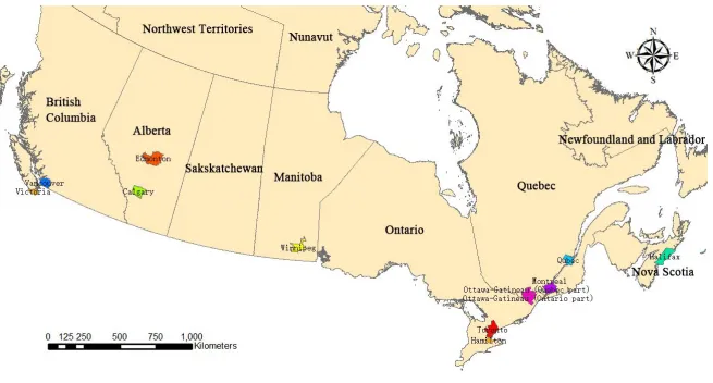
In particular, part of this thesis (Chapter 2) uses Sentinel-2 satellite imageries. Sentinel-2 is a monitoring mission from the EU Copernicus plan, and it consists of two identical satellites, Sentinel-2A and Sentinel-2B. The first satellite, Sentinel-2A, was launched in June 2015 and Sentinel-2B was launched on March 7, 2017. Each satellite carries a multi-spectral instrument (MSI) with 13 multi-spectral bands. Since Sentinel-2 can provide relatively high-spatial resolution (10 m to 60 m) imagery, it is viewed as an important source for future applications in remote sensing. In the present study, Sentinel-2 data combined with conventional Landsat 5 satellite data (Chapter 3) are used to examine urban boundary expansion. The satellite imageries are matched with residents’ socioeconomic data from the corresponding census, forming a data set based on Dissemination Areas (DAs) for the 11 most populous CMAs in Canada, namely Toronto, Montreal, Vancouver, Calgary, Ottawa–Gatineau, Edmonton, Quebec City, Winnipeg, Hamilton, Halifax, and Victoria.
helps provide a first-step systematic and precise analysis of what causes urban sprawl in terms of urban boundary expansions away from the city core. Doing so also allows one to leverage on the long-standing, well-established urban economic theories about urban development. Essentially, the monocentric city model (Alonso, 1964; Muth, 1969; Mills, 1967) and the Tiebout model (Tiebout, 1956) have laid the groundwork and served as the theoretical framework for the analysis.
To be specific, indeed, many studies that have attempted to explain urban sprawl (Brueckner & Fansler, 1983; Burchfield, Overman, Puga, & Turner, 2006; McGrath, 2005; Oueslati, Alvanides, & Garrod, 2015) originate from two branches of theories: the monocentric city model and the Tiebout model. The monocentric city model assumes that a city’s spatial size is determined by population, income, agricultural land rent, and commuting costs. According to Wheaton (1974), who has provided a thorough
comparative analysis of the monocentric model, urban boundary expands with population and income, but contracts with increasing agricultural land rent and transportation costs. The Tiebout model, on the other hand, assumes residents may “vote by their feet” —that is residents move to locations with public services that meet their preferences. In its original formulation, the Tiebout model has several assumptions. First, residents are free to move across communities and have perfect information about local services. Second, there are enough communities that can meet residents’ preferences. Third, the model assumes that there are no externalities or spillover of public goods across municipalities. This relationship between urban sprawl and public services has been examined and verified by a number of empirical studies (Carruthers & Ulfarsson, 2003; Dowding, John, & Biggs, 1994).
policy uncertainties, some others could be developer-specific, related to the developer’s own financial risk. This empirical studies adopt a simple approach and focus on the total risk only—the sum of the systematic and unsystematic risk—as reflected in the price variance. Re-inserting this role into the existing theories helps researchers and policy makers in better understanding why certain growth policies might work and why some others are ineffective—this is one of the objectives and contributions of the two empirical studies.
The public data from Canadian census are not readily available for conducting long-term longitudinal studies—that is, it is not a straightforward task to determine and assess land use/cover changes over time. Allen and Taylor (2018) have developed an innovative set of bridging data that can be applied to Census Tracts (CT) over the years, using the combination of dasymetric areal interpolation and population weighting methods. Following Allen and Taylor’s method, Chapter 3 focuses on smaller units, which are Dissemination Areas (DAs) and Enumeration Areas (EAs) and conduct boundary reconciliation and data reallocation for 1986, 2006, and 2016 (Chapter 3).
In sum, this dissertation presents two studies that empirically examine the causes of urban sprawl. The first paper focuses on 11 Canadian CMAs and tests the traditional theories of urban sprawl, the monocentric city model and the Tiebout model, using cross-sectional data in 2016. The second paper zooms into the largest CMA in Canada, Toronto, and examines the longitudinal changes in the urban coverage at the fringe. Land cover/use changes in the Toronto CMA for 1986-2006 and 2006-2016 are detected using remote-sensing techniques. Both papers are innovative in that they attempt to broaden the existing theories by inserting the role of price risk to the understanding of the timing of urban development. In particular, both papers seek to provide an empirical analysis of how price risk influences the extent and the timing of urban development from the developer’s perspective.
1.2
Research objectives
1. To refine previous studies by adopting a more precise delineation of urban coverage for statistical analysis of urban sprawl. Built-up areas extracted from land cover/use maps are used based on Sentinel-2 satellite imageries for the 11 CMAs in 2016 instead of using census data.
2. To detect changes in the land cover/use patterns for the Toronto CMA using a
combination of Sentinel-2 and Landsat 5 satellite imageries from 1986, 2006, and 2016 at the DA (or EA) level.
3. To test the monocentric city model and the Tiebout model using the 11 most populous CMAs in Canada and particularly the Toronto CMA.
4. To fill in the research gap by inserting the role of price risk and, specifically, the availability of the real option, in affecting the speed of urban sprawl. The dissertation challenges the efficacy of contemporary urban growth policies: They focus mostly on the demand and supply side of growth, but have ignored important market factors such as price risks. Once price risks have been taken into account, developers do consider the timing of their development, thereby affecting both the extent and the speed of urban sprawl.
1.3
Study area and data
Chapter 2 examines the 11 most populous Canadian CMAs: Toronto, Montreal,
Vancouver, Calgary, Ottawa—Gatineau, Edmonton, Quebec City, Winnipeg, Hamilton, Halifax, and Victoria (Figure 1.1). It focuses on these CMAs because of data availability: The study requires the use of price indices to construct the risk variable. Price indices are available for these CMAs only. According to Statistics Canada, a CMA is defined as an area that is formed by one or more adjacent municipalities located around a core
(Statistics Canada, 2016). A CMA must have a total population of at least 100,000. The spatial vastness of a CMA implies that its boundary often encompasses the boundary of a city; the latter is defined politically by the city government.
Data used in this study can be generally categorized as two types: remote-sensing data and census data.
Landsat 5 was launched on March 1, 1984 and was a low Earth orbit satellite for collecting imagery, with the multi-spectral bands’ resolution of up to 30 m. It is widely used to study climate change, agricultural practices, and the development of cities (Earth Observing System, 2012). Along with the technical progress, a new generation of high spatial-resolution satellite imagery makes it possible to widen the application of satellite imagery—for example, Sentinel-2 is a “Landsat-like” observatory from the Copernicus Programme of the European Space Agency (ESA). It achieves five-day repeat period with two twin satellites, S2A and S2B. S2A was launched on June 23, 2015, while S2B was launched on March 7, 2017. In the present study, only S2A data are used. Compared to the sensors of Landsat 5, those of Sentinel-2 have more spectral bands (i.e., 13 for Sentinel-2 sensors versus 7 for Landsat 5 sensors) and higher spatial resolution, which is up to 10 meters. The spatial resolution of main visible and near-infrared Sentinel-2A bands is 10 m, and that of red, near-infrared and two shortwave infrared bands is 20 m. The coastal/aerosol, water vapor, and cirrus bands have a spatial resolution of 60 m. Landsat 5 TM and ETM+ satellite imageries from 1986 and 2005 and Sentinel-2 data of 2016 were collected and used in this study. High-resolution imageries from Google Earth were also acquired as reference maps for selecting training samples and testing samples during image classification.
1.4
Thesis organization
The research is presented in the integrated-article format. Chapters 2 and 3 are written independently, tailored for submissions to peer-reviewed journals.
The thesis is structured as follows. Chapter 1, Introduction, presents a brief overview of the dissertation. It reviews the theories and previous studies related to this research. It states the objectives and defines the study area as well as the data used in the dissertation.
Chapter 2 is the first of the two integrated papers. It presents a cross-sectional
comparison among the 11 most populous CMAs in Canada in terms of their extent of urban sprawl. It examines the two traditional theories of urban sprawl: the monocentric city model and the Tiebout model. It also studies the role of price risk in affecting the extent of urban land cover/use changes in developable land outside of cities.
Chapter 3 is the second of the two integrated papers. It presents a longitudinal case study of the Toronto CMA. It employs the difference-in-difference model to study how price risk might have affected both the extent and the timing of urban land cover/use changes outside of the city in the Toronto CMA.
Chapter 4 provides a summary of the results, followed by a discussion of the contributions to the literature. It also presents the limitations of this research and suggestions for future research.
1.5
References
Allen, J., & Taylor, Z. (2018). A new tool for neighbourhood change research: The Canadian Longitudinal Census Tract Database, 1971–2016. The Canadian
Geographer/Le Géographe canadien, 62(4), 575-588.
Alonso, W. (1964). Location and land use. Toward a general theory of land rent.
Location and land use. Toward a general theory of land rent.
Burchfield, M., Overman, H. G., Puga, D., & Turner, M. A. (2006). Causes of Sprawl: A Portrait from Space. The Quarterly Journal of Economics, 121(2), 587-633. doi:10.1162/qjec.2006.121.2.587
Carruthers, J. I., & Ulfarsson, G. F. (2003). Urban Sprawl and the Cost of Public Services. Environment and Planning B: Planning and Design, 30(4), 503-522. doi:10.1068/b12847
Dowding, K., John, P., & Biggs, S. (1994). Tiebout: A survey of the empirical literature.
Urban studies, 31(4-5), 767-797.
Dupras, J., Alam, M., & Revéret, J. P. (2015). Economic value of Greater Montreal's non‐market ecosystem services in a land use management and planning
perspective. The Canadian Geographer/Le géographe canadien, 59(1), 93-106.
Earth Observing System. (2012). LANDSAT 5 (TM). Retrieved from https://eos.com/landsat-5-tm/
Eidelman, G. (2010). Managing urban sprawl in Ontario: good policy or good politics?
Politics & Policy, 38(6), 1211-1236.
Feng, L., Du, P. J., Li, H., & Zhu, L. J. (2015). Measurement of Urban Fringe Sprawl in Nanjing between 1984 and 2010 Using Multidimensional Indicators:
Measurement of Urban Fringe Sprawl. Geographical Research, 53(2), 184-198. doi:10.1111/1745-5871.12104
Filion, P. (2003). Towards smart growth? The difficult implementation of alternatives to urban dispersion. Canadian Journal of Urban Research, 12(1), 48.
Furberg, D., Ban, Y., Geodesi och, g., Kth, Samhällsplanering och, m., & Skolan för arkitektur och, s. (2012). Satellite Monitoring of Urban Sprawl and Assessment of its Potential Environmental Impact in the Greater Toronto Area Between 1985 and 2005. Environmental Management, 50(6), 1068-1088. doi:10.1007/s00267-012-9944-0
Galster, G., Hanson, R., Ratcliffe, M. R., Wolman, H., Coleman, S., & Freihage, J. (2001). Wrestling sprawl to the ground: defining and measuring an elusive concept. Housing policy debate, 12(4), 681-717.
Hu, Q., Wu, W., Xia, T., Yu, Q., Yang, P., Li, Z., & Song, Q. (2013). Exploring the Use of Google Earth Imagery and Object-Based Methods in Land Use/Cover
Mapping. Remote Sensing, 5(11), 6026-6042. doi:10.3390/rs5116026
Jat, M. K., Garg, P. K., & Khare, D. (2008). Monitoring and modelling of urban sprawl using remote sensing and GIS techniques. International Journal of Applied Earth
Observation and Geoinformation, 10(1), 26-43.
McGibany, J. (2004). Gasoline prices, state gasoline excise taxes, and the size of urban areas. Journal of Applied Business Research.
McGrath, D. T. (2005). More evidence on the spatial scale of cities. Journal of Urban
Economics, 58(1), 1-10.
Miron, J. (2003). Urban sprawl in Canada and America: Just how dissimilar. University
of Toronto, Department of Geography, Toronto.
Oueslati, W., Alvanides, S., & Garrod, G. (2015). Determinants of urban sprawl in European cities. Urban Studies, 52(9), 1594-1614.
Song, Y., & Zenou, Y. (2006). Property tax and urban sprawl: Theory and implications for US cities. Journal of Urban Economics, 60(3), 519-534.
Statistics Canada. (2016). Dictionary, Census of Population, 2016. Retrieved from https://www12.statcan.gc.ca/census-recensement/2016/ref/dict/index-eng.cfm
Statistics Canada. (2017). Census in Brief: Municipalities in Canada with the largest and fastest-growing populations between 2011 and 2016. Retrieved from
https://www12.statcan.gc.ca/census-recensement/2016/as-sa/98-200-x/2016001/98-200-x2016001-eng.cfm
Sun, H., Forsythe, W., & Waters, N. (2007). Modeling Urban Land Use Change and Urban Sprawl: Calgary, Alberta, Canada. Networks and Spatial Economics, 7(4), 353-376. doi:10.1007/s11067-007-9030-y
Sutton, P. C. (2003). A scale-adjusted measure of “urban sprawl” using nighttime satellite imagery. Remote sensing of environment, 86(3), 353-369.
Tiebout, C. M. (1956). A pure theory of local expenditures. Journal of political economy, 64(5), 416-424.
Wheaton, W. C. (1974). A comparative static analysis of urban spatial structure. Journal
of Economic Theory, 9(2), 223-237.
2
Testing Theories of Urban Sprawl Using Sentinel-2
Imagery: A Cross-sectional Comparison among 11
Canadian Census Metropolitan Areas
2.1
Introduction
2.1.1
Background
Sprawl is among the most important issues facing contemporary cities. The issue has been placed on the national agenda, with the Canadian federal government calling for research on growth management policies to guide the “smart growth” of cities (Policy Horizons Canada, 2016). Strong sentiment against sprawl has developed over the last decade in North American cities. At the root of this sentiment are a number of problems associated with “unmanaged” urban growth (Alexander & Tomalty, 2002; Daniels, 2001; Filion, 2003). Cities encroach excessively on agricultural land, leading to a loss of open space and farmland. Urban expansion implies longer commutes, generating traffic congestion and air pollution. Low-density suburban developments increase residents’ reliance on automobiles, potentially contributing to obesity due to a lack of physical exercise. Scattered developments cost more in terms of municipal services. A large number of studies have assessed the economic and environmental costs of sprawl and recommended policies to better manage urban growth; however, little has been done to document systematically the process and extent of sprawl. Knowing exactly the location and the extent of urban boundary changes are important, as they provide a basis for designing smart growth policies and for anticipating changes in financing and servicing the expansion. The objective of this study is to fill this research gap, using 11 Canadian Census Metropolitan Areas (CMAs) as comparative case studies, namely Toronto, Montreal, Vancouver, Calgary, Ottawa–Gatineau, Edmonton, Quebec City, Winnipeg, Hamilton, Halifax, and Victoria.
areas outside of cities. Urban land coverage is measured as the amount of built-up land area in the fringe of the 11 CMAs. This definition excludes protected areas such as the greenbelt (see Appendix A). Note that the boundary of the greenbelt (mainly in Toronto and Ottawa) has remained stable over the last 30 years.
The present study differs from those in the past (Carruthers & Ulfarsson, 2003; Oueslati, Alvanides, & Garrod, 2015) in that it focuses on the urban extent in terms of urban land cover and land use. Census data have usually been used to form sprawl indices in past studies. The emergence of satellite imagery has provided a new method for monitoring land cover/use changes (Alberti, Weeks, & Coe, 2004). The combination of remote sensing and geographic information science (GIS) techniques can add details to the detection of land cover/use changes.
Traditional theories that explain urban sprawl stem mostly from two branches: the monocentric city model (Alonso, 1964; Muth, 1969; Mills, 1967) and the Tiebout model (Tiebout, 1956). The monocentric city model focuses on changes associated with the residents, such as changes in income and transportation costs. Based on the monocentric city model, existing empirical studies mostly find consistent evidence supporting the theory: increases in population and household incomes induce a higher demand for urban areas thereby causing urban boundaries to expand; urban boundaries shrink as the
commuting costs and agricultural land rent increase (Brueckner & Fansler, 1983; Gao, Kii, Nonomura, & Nakamura, 2017; McGrath, 2005; Oueslati, Alvanides, & Garrod, 2015). It is arguable that one can hardly find, in reality, contemporary cities with only one employment center, thereby rendering the monocentric city model inapplicable. However, the monocentric city model is the starting point for understanding the crude, discrete location choices of in-versus-outside of the city, a simple application that allows the researcher to use the model to study urban sprawl.
development and public services (Carruthers & Ulfarsson, 2003; Dowding, John, & Biggs, 1994).
What is missing in the literature is the role of price risk, which refers to uncertain future prices of housing. Focusing on price risk requires the researcher to adopt the developer’s perspective when studying the timing of urban development. Price risk has at least two opposing forces on the timing decision—in terms of the developer’s risk aversion and of the availability of the real option. The former favors more instantaneous developments at the present time; the latter creates incentives for developers to delay. Reinserting the role of price risk in understanding urban sprawl helps policy makers in formulating more informed and timely growth policies in light of market conditions.
Note that, here, price risk refers to the total risk observed in transacted prices. Ideally, one would like to separate the total risk into systematic, market risk versus non-systematic, developer-specific risk. The former might be related to general market uncertainties such as interest rate and policy uncertainties. The latter could refer to the financing and business risk confronted by individual developers. However, one cannot find specific variables to help separate the two types of risk; therefore, this study focuses on the two types combined, as reflected in the variance and the coefficient of variation of transacted prices.
developers. They show that risk has a negative impact on the extent of urban
development in the fringe: developers tend to delay development due to the presence of the real option.
2.1.2
Previous studies and theories
The monocentric city model focuses on the result of a competitive bidding process of location choice. The model assumes perfect mobility among homogeneous residents, who live on a featureless plain and compete for proximity to a central workplace. At the equilibrium, those residents who move away from the central business district (CBD) save housing rent, but at the same time incur higher commuting costs—that is, higher commuting costs are completely offset by lower housing rents within the monocentric city model.
Wheaton (1974) has provided a thorough set of comparative static analysis for the monocentric city model:
0, 0, 0, 0
a
x x x x
n t y r
(2.1)
where x is the distance to the CBD; n is the total urban population; t is the one-way commuting cost per mile; y is annual income, and 𝑟𝑎is the agricultural land rent in areas outside of a fixed city boundary. Wheaton’s analysis shows that the urban boundary x expands with population and income, but contracts with rising agricultural land rent and commuting costs.
concludes that the monocentric city model is empirically robust. Young, Tanguay, and Lachapelle (2016) conduct a study on 10 CMAs between 1996 and 2011. Their results show that gasoline fees have more significant effects on urban sprawl than off-street parking fees. The authors agree that higher transportation costs can restrain the extent of sprawl. The present study follows Brueckner and Fansler and uses cross-sectional data to examine the role of the monocentric city model and the Tiebout model in explaining urban sprawl in the 11 Canadian CMAs.
Unlike the monocentric city model, The Tiebout model focuses on the supply of public goods and services and residents’ choices of public goods in terms of their preferences—
that is, residents tend to move to locations that offer public goods that meet their
preferences and “vote by their feet” (Tiebout, 1956). Carruthers and Ulfarsson (2003) use various prices of municipal services as proxies for the Tiebout model and show that the relative strength of the property tax base can lead to the sprawling of a metropolitan area. The present study follows but modifies Carruthers and Ulfarsson, by using property tax rates to study the extent to which pricy municipal public goods might be positively related to more urban development in sprawling areas.
Both the monocentric city and Tiebout models ignore the developer’s view of
development on the fringe, especially in light of price risk. Consider a developer who confronts uncertain future price (return) of the development. The developer needs to decide when to develop—either now or the future—in light of discounted benefits with the presence of price (return) risk. Price risk exerts three impacts on the timing decision. First, if the developer is risk-averse, price risk creates an incentive for the developer to build now as opposed to confronting the risk in the future.
Third, the presence of the real option lessens the downside price risk and increases the net present value (NPV) from delaying development. Put differently, if the developer owns the land, he or she has an additional option to delay developing the land and earn the agricultural land rent if the price drops in the future, thereby obviating the need to take a loss. The NPV with real option is, therefore, greater than that without. This higher NPV creates an incentive for the developer to delay.
In sum, the present study uses 11 CMAs in Canada to test the theories of the monocentric city model and the Tiebout model. It contributes to the literature by inserting the role of the developer in light of price risk, that is, how price risk could delay or speed up urban sprawl.
2.2
Data and variables
2.2.1
Study Area
This study focuses on the 11 most populous CMAs in Canada: Toronto, Montreal, Vancouver, Calgary, Ottawa–Gatineau, Edmonton, Quebec City, Winnipeg, Hamilton, Halifax, and Victoria. Statistics Canada defines a CMA as an area consisting of at least one municipality located around a core city, which also includes a population of at least 100,000 (Statistics Canada, 2016). Given the vastness of its spatial scale, a CMA is usually greater in area than a city, with the latter defined mostly politically by the city government.
The unit of analysis in this study is the dissemination area (DA). A DA is a small
geographic area which contains 400 to 700 people. It is the smallest standard geographic unit for Statistics Canada to partition the national map and disseminate census
information.
2.2.2
Data
Landsat, Sentinel-2 has more spectral bands and higher spatial resolution (see details in Table 2.1). It can provide more useful and accurate information for land cover/use classification. Data acquisition dates are shown in Table 2.2.
Table 2. 1 Details of the Sentinel-2 spectral bands
Band name
S2A S2B Spatial
resolu-tion (m) Central wavelength (nm) Bandwidth
(nm) wavelength Central (nm)
Bandwidth (nm)
1 aerosol Costal 442.7 21 442.2 21 60 2 Blue 492.4 66 492.1 66 10 3 Green 559.8 36 559.0 36 10
4 Red 664.6 31 664.9 31 10
5 Vegetation red edge
704.1 15 703.8 16 20
6 Vegetation red edge 740.5 15 739.1 15 20
7 Vegetation red edge
782.8 20 779.7 20 20
8 NIR 832.8 106 832.9 106 10 8A Narrow
NIR
864.7 21 864.0 22 20
9 vapour Water 945.1 20 943.2 21 60
10 SWIR – Cirrus 1373.5 31 1376.9 30 60 11 SWIR 1613.7 91 1610.4 94 20 12 SWIR 2202.4 175 2185.7 185 20
Table 2. 2 Sentinel-2 data acquisition dates (year=2016)
Training samples and testing samples are used to process classification and estimate classification accuracy, separately. Google Earth imageries for corresponding dates in 2016 are used as reference maps to choose these samples randomly for each class.
Second, the study uses Statistics Canada’s boundary and census data that are publicly available. The pixels from the classified Sentinel imageries are aggregated to match the boundaries of the 2016 DA of the corresponding CMA. The boundary data for DAs and CMAs are drawn from Statistics Canada’s cartographic boundary files. The aggregated socioeconomic characteristics of DA residents are obtained from the 2016 census profile series. As shown in Table 2.3, census data for the DAs include total population, median income, number of dwellings, median value of dwellings, and median monthly rent. All dollar values are measured in the 2016 Canadian dollar.
CMA name Date
Toronto September 24
Montreal July 20
Vancouver August 29
Calgary August 30
Ottawa–Gatineau June 23
Edmonton May 2
Quebec City September 5
Winnipeg September 8
Hamilton September 24
Halifax June 18/August 31
Table 2. 3 Census data definition
Name Description
DAUID The unique identifier for each DA Population Total population in the DA
Dwelling No. of private dwellings occupied by usual residents in the DA Med_income Median total income ($) in the DA
Med_dwelling Median value of dwellings ($) in the DA Med_rent Median monthly rent ($) in the DA
Source: 2016 Canadian census profile series for Dissemination Areas
Third, municipal property tax rates are assembled. Ideally, municipal services or
Table 2. 4 Mill rate for the 11 Census Metropolitan Areas in 2016
CMA Name Property tax rate
Hamilton 0.0137
Halifax 0.0121
Winnipeg 0.0118
Ottawa 0.0105
Montreal 0.0099
Quebec City 0.009
Edmonton 0.008
Toronto 0.0069
Victoria 0.0068
Calgary 0.0062
Vancouver 0.0032
Source: Municipal websites and services
Notes: Some CMAs comprise more than one municipalities/cities—for example, the
Toronto CMA has at least nine major cities: the city of Toronto, Oakville, Mississauga, Ajax, Pickering, Whitby, Richmond Hill, Markham, Vaughan, and some other smaller municipalities. The present study uses the mill rate from only the largest, core city in the CMA, such as the city of Toronto, as a proxy for the centrifugal force that drives
residents away from the pricy locations to more outer areas of a CMA. For this reason, the study does not model the intra-CMA residential mobility and tends to underestimate the Tiebout forces that might have led to the previously sprawled areas.
The regression model, which is a cross-section analysis, compares the extent to which the within-CMA Tiebout effects might vary across the 11 CMAs.
period in this study is January 2006 to December 2016. By far, this is the best and the most available index for calculating price risk.
Figure 2.1 shows the HPI of the 11 CMAs (June 2005=100) and Table 2.5 summarizes the indices. Almost all CMAs demonstrated steady price growth between 2006 and 2016.
Figure 2. 1 House Price Indices of the 11 Canadian Census Metropolitan Areas from
January 2006 to December 2016
Notes: c6 refers to Victoria, Vancouver, Winnipeg, Montreal, Quebec City, and Halifax;
and c11 refers to the above six CMAs plus Calgary, Edmonton, Hamilton, Toronto, and Ottawa.
The summary statistics presented in Table 2.5 show that the average HPI of the 11 CMAs is 147.1, with a standard deviation of 23.0. Vancouver, Winnipeg, and Toronto
Table 2. 5 Summary statistics of House Price Indices
CMA
Name Min. Mean Max. Std. Dev. CV
a
Victoria 106.09 139.51 176.78 11.28 0.081 Vancouver 107.16 164.89 249.53 31.13 0.189 Calgary 108.45 163.40 188.35 15.74 0.096 Edmonton 105.57 166.18 187.91 17.19 0.103 Winnipeg 103.67 167.25 204.03 29.59 0.177 Hamilton 102.89 134.52 201.47 24.43 0.182 Toronto 102.21 138.48 216.53 28.94 0.209 Ottawa 101.15 129.31 147.49 14.62 0.113 Montreal 99.96 136.86 160.47 17.73 0.130
Quebec
City 102.06 152.88 183.19 26.82 0.175 Halifax 100.98 128.93 143.90 12.33 0.096 6 cities 103.51 146.03 203.32 24.09 0.165 11 cities 103.65 147.06 200.69 23.02 0.157
Source: Teranet–National Bank House Price Index (n=132)
Notes: aCV=Std. Dev.
Mean
Fifth, the urban boundaries for each CMA in 2006 are also drawn from Statistics Canada. To focus on urban sprawl, this study is limited only to developable land outside of the city in each CMA. Statistics Canada defines an urban area (UA) as a community with at least 1,000 people and a population density of at least 400 persons per square kilometer. This definition has remained unchanged since 2006.
2.2.3
Variables
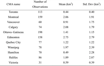
The dependent variable is the built-up area in the DAs, which are within the CMA but lie outside of the city and which do not encroach on any greenbelt restricted areas. These DAs are, henceforth, referred to as the developable DAs. Four land cover/use types are reclassified as built-up area: residential, industrial, transportation, and golf. Table 2.6 shows a summary of the dependent variable for the 11 CMAs.
Table 2. 6 Summary statistics of the dependent variable (built-up area in the
Dissemination Area) for each Census Metropolitan Area
CMA name Number of
Observations Mean (km
2) Std. Dev (km2)
Toronto 113 0.44 0.40
Montreal 159 2.06 1.91
Vancouver 60 0.91 1.75
Calgary 74 2.08 1.79
Ottawa–Gatineau 198 1.41 1.15
Edmonton 158 2.75 2.79
Quebec City 77 1.22 1.22
Winnipeg 78 1.97 2.39
Hamilton 70 0.49 2.28
Halifax 86 1.89 2.87
Victoria 31 0.59 0.39
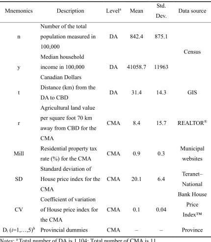
Table 2. 7 Statistical summaries of the independent variables
Mnemonics Description Levela Mean Std.
Dev. Data source
n
Number of the total population measured in 100,000
DA 842.4 875.1
Census
y
Median household income in 100,000 Canadian Dollars
DA 41058.7 11963
t Distance (km) from the
DA to CBD DA 31.4 14.3 GIS
r
Agricultural land value per square foot 70 km away from CBD for the CMA
CMA 8.4 15.7 REALTOR®
Mill Residential property tax
rate (%) for the CMA CMA 0.9 0.3
Municipal websites
SD
Standard deviation of House price index for the CMA
CMA 20.1 6.4 Teranet– National Bank House
Price Index™ CV
Coefficient of variation of House price index for the CMA
CMA 0.1 0.04
Di (i=1,…,5)b Provincial dummies CMA – – Province
Notes: a Total number of DA is 1,104; Total number of CMA is 11.
b Alberta is taken as the reference. The identifier i represents Ontario, British Columbia,
Manitoba, Quebec, and Nova Scotia, respectively.
which is calculated as the SD divided by the mean of the CMA’s price index in the time period.
To model the monocentric city model, four variables are used: population, income, agricultural land value, and distance to the Central Business District (CBD). The agriculture land rent is proxied by agricultural land value per square foot 70 km away from CBD for each CMA. This value is obtained from the current Multiple Listing Services. The agricultural land rent is an approximation, and 70 km is a crude
measurement to find a realistic piece of agricultural land. Following the monocentric city model, it is assumed that agricultural land rent is flat everywhere outside of the city. Note that the study previously attempted to use corn prices as a proxy for measuring
agricultural land rent, but the results were not satisfactory; therefore, MLS land rent is employed instead.
Commuting cost is proxied by the distance between the geometric center (the centroid) of each DA and the CBD. Since most job opportunities centralize in the CBD, residents can live close to the center to reduce commute time, thereby lowering the costs for
commuting. To model the polycentric aspects of the CMAs, the study attempted to include distance variables to other secondary employment centers; however, these additional distance variables were mostly insignificant, while, at the same time, created multicollinearity into the regression model. For this reason, this study excludes them from the estimation.
The cities’ mill rates are used to model for the Tiebout effect. It is expressed as dollar amount of property tax payable per $1,000 of assessed property value.
2.3
Methods and Empirical Strategy
2.3.1
Data Pre-processing
Transverse Mercator (UTM) coordinate system and the World Geodetic System (WGS-1984).
The Smoothing Filter-based Intensity Modulation (SFIM) technique (Liu, 2000) is used to enhance the spatial details without altering the spectral properties. SFIM is an image fusion method to fuse lower spatial-resolution multispectral bands with higher-resolution bands. A ratio between a higher resolution image and its low-pass mean filtered image was used to modulate a lower spatial-resolution multispectral image without changing its spectral properties. The SFIM is defined as
low high
fus
mean
DN( ) DN( ) DN( )
DN( )
= (2.2)
where DN(λ)fus, DN(λ)low, DN(γ)high, DN(γ)mean are DN values of fused higher spatial
resolution image, original low spatial resolution image, original high spatial resolution panchromatic image, low spatial resolution panchromatic image (after applying the low-pass filtering in the original panchromatic image), correspondingly. Since Sentinel-2 satellite imagery does not include panchromatic bands, relatively higher-resolution red bands were used during the image fusion process. Compared to the original imagery, fusion imagery provides more spatial details. After image fusion, all generated bands were processed using the layer stacking method to obtain layers for classification. Finally, the seamless mosaic workflow in ENVI 5.3 was used to combine adjacent imageries with color balance. The mosaicked image was then clipped by the boundary of the corresponding CMA.
2.3.2
Image Classification
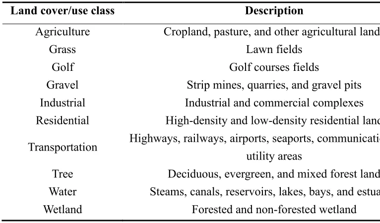
After pre-processing, the supervised maximum likelihood classification (MLC) method was used to obtain the land cover/use maps. Land cover/use types were classified into ten classes (Table 2.8), which were based on the land cover/use classification system
Table 2. 8 Land cover/use classification scheme
Land cover/use class Description
Agriculture Cropland, pasture, and other agricultural lands
Grass Lawn fields
Golf Golf courses fields
Gravel Strip mines, quarries, and gravel pits Industrial Industrial and commercial complexes Residential High-density and low-density residential land
Transportation Highways, railways, airports, seaports, communications, and utility areas
Tree Deciduous, evergreen, and mixed forest land Water Steams, canals, reservoirs, lakes, bays, and estuaries Wetland Forested and non-forested wetland
In this study, the Maximum Likelihood Classifier (MLC) method was used to process classification because it performs well when studying land cover/use change (Otukei & Blaschke, 2010). The way MLC works is that it supposes the pixels in each class are normally distributed; each pixel is assigned to the class with the greatest maximum likelihood value (Scott & Symons, 1971).
2.3.2.1
Classification Accuracy Assessment
2.3.2.2
Post-classification Processing
The built-up area in each DA was defined in two ways. The first way was the measured amount of land area that is built-up in the DA. The second way treated built-up area as a dichotomous variable: it was a one if built-up area is the single largest land-cover/use class in the DA and a zero otherwise. In the latter case, zonal statistics method was applied to identify the predominant land cover/use type in each DA. This step ensured the unit of observation from satellite imagery matches with census unit. In the regression model, the dependent variable is the actual measurement of the built-up area.
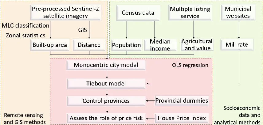
2.3.3
Empirical Strategy
Figure 2.2 shows the conceptual diagram relating theories, data, and methods. Using the MLC classification and zonal statistics, all land cover/use types in the DA are identified. The land cover/use data are then matched with the census socioeconomic variables, which are aggregated data at the DA level. A list of datasets with all attributes is
imported to R for estimating the regression model, based on the Ordinary Least Squares (OLS) method.
The estimating regression equation between the dependent variable and independent variables is given as follows:
5
0 1 2 3 4 5 , , 6 7
1
ij ij ij ij i i k i j k i i ij
k
p n y t r Mill d SD CV
=
= + + + + + +
+ + + (2.3)where i and j represent provinces and CMAs, respectively; p (the dependent variable)is the amount of built-up land area in 2016; n represents population; y is median income; t is the proxy for commuting costs; r stands for agricultural land value; Mill refers to the mill rate; d stands for regional dummies (British Colombia, Manitoba, Quebec, Nova Scotia, and Ontario; Alberta is the referenced region); SD and CV are the standard deviation and the coefficient of variation of the House Price Index, correspondingly, and ij is the error
term. The errors are assumed to independent and identically distributed as normal.
One might argue that urban developments might exhibit the “spillover effect” in that new developments tend to cluster around developed land to be cost effective in serving land. In this case, the OLS model fails to capture the spillover effect; instead, one should estimate a spatial regression model either in the form of spatial lag, spatial error, or a combination of both. However, estimating a spatial model is beyond the scope of the present study; the next phase of the research beyond the dissertation would include testing and estimating spatial models.
2.4
Results and Discussion
2.4.1
Land Cover/Use Estimates
The land cover/use maps of 11 CMAs are generated using the zonal statistics method. As an example, Figure 2.3 shows the result for all the 11 CMAs.
(a) Toronto, Montreal, and Vancouver CMAs
(c) Winnipeg, Halifax, Hamilton, and Victoria CMAs
Figure 2. 3 (a) (b) (c) Land cover/use patterns for the 11 Census Metropolitan Areas
using zonal statistics
As shown in Table 2.9, the overall classification accuracy for the 11 CMAs ranges between 82.3 and 94.7%. The Montreal CMA shows the lowest accuracy, 82.3%, with a Kappa coefficient of 0.80, and the highest accuracy is the Edmonton CMA (94.7%), with a Kappa coefficient of 0.94.
Table 2. 9 Accuracy assessment
CMA name Overall accuracy Kappa coefficient
Toronto 86.54% 0.85
Montreal 82.30% 0.80
Vancouver 88.93% 0.88
Calgary 90.62% 0.90
Ottawa-Gatineau 88.39% 0.87
Edmonton 94.68% 0.94
Quebec City 88.00% 0.87
Winnipeg 90.50% 0.89
Hamilton 84.29% 0.82
Halifax 91.77% 0.91
2.4.2
Statistical Analysis
The OLS regression results of the five models are presented in Table 2.10. The dependent variable is the measurement of built-up land area in the DA.
Model 1 focuses on the traditional monocentric city model. Its independent variables include population, income, agricultural land rent, and commuting costs. As expected, the coefficients of median income and agricultural land value show significant positive and negative impacts, respectively.
Model 2 expands the monocentric city model to include the Tiebout model; in model 3, the regional dummies are also further included to control for any unobserved influences at the provincial level. Models 4 and 5 include two different measurements of price risks, SD and CV. As expected, the coefficients of population, income, commuting costs, mill rate, and price risk are highly significant, as indicated by the small p-values (<0.1).
The main results show that risk is significant in affecting the amount of land developed at the fringe of a city. In models 4 and 5, both risk variables are positive and significant. Consider the impact of price risk on urban land coverage outside of the cities. On average, a 1% point increase in the CV of the house price index is associated with close to 10 square kilometers less built-up areas in the fringe. It conforms with the theory that price risk slows down urban development—that is, risks might create an incentive for developers to delay development due to the presence of the real option, an option that hedges the risk of a price decline for the developer.
Table 2. 10 OLS estimation results (n=1,104)
Model 1 Model 2 Model 3 Model 4 Model 5
Intercept -0.513
* (1.90) -0.637 (1.61) -1.937*** (4.52) -0.381 (0.67) -0.282 (0.51)
n 0.076 (0.12) 0.099 (0.16) 1.489** (2.42) 1.607*** (2.63) 1.658*** (2.72)
y 15.463
*** (3.18) 15.453*** (3.18) 11.835** (2.47) 8.892* (1.85) 8.197* (1.70)
r -2.477
*** (7.12) -2.389*** (5.93) -0.03 (0.05) 1.076 (1.63) 0.983 (1.54)
t 5.339
*** (13.45) 5.381*** (13.16) 5.873*** (14.60) 5.710*** (14.23) 5.737*** (14.35)
Mill – 0.112
(0.43) 2.540*** (6.77) 1.857*** (4.55) 1.818*** (4.50)
D1 – –
-2.131*** (10.90) -1.876*** (9.20) -1.573*** (6.88)
D2 – –
-1.179*** (6.41) -0.871*** (4.40) -0.669*** (3.13)
D3 – –
-0.749** (2.09) -1.122*** (3.06) -1.023*** (2.84)
D4 – –
-1.405*** (5.11) -0.450 (1.25) -0.406 (1.16)
D5 – –
-1.395*** (5.04) -1.332*** (4.84) -1.129*** (4.03)
SD – – –
-0.052***
(4.09) –
CV – – – –
-9.192***
(4.59) Adjust R2 0.163 0.162 0.251 0.262 0.265
Notes: The dependent variable is built-up area in square kilometer in the DA. The
***, **, * represent the coefficient is significant at the 1%, 5%, 10% level, correspondingly,
with two-tailed tested.
The variations in the independent variables explain about 16% (Model 1) of the variation in the dependent variable. In particular, the risk variable increases the explanatory power of the model by about 10%, to a relatively higher R-square of 26.5% (Model 5).
2.5
Conclusions
This study mixes remote-sensing and GIS with empirical techniques to test the causes of urban sprawl in light of price risk. It demonstrates that Sentinel-2 satellite imagery can provide useful information for land cover/use classification. From the classification results, built-up areas can be explored for studying urban sprawl with high accuracy. The combination of remote sensing measures and census data adds details to the analysis of urban sprawl since the two types of information cannot substitute for each other.
The results show that the relationships between urban coverage and population, and between urban coverage and the mill rate are consistent with the traditional theories in the urban fringe area of the 11 CMAs in which urban sprawl can potentially happen. The analysis shows that urban sprawl is positively related to population, income, and the mill rate. In the case of the Tiebout model, the positive coefficient of mill rate is logical: higher prices for similar public goods might push residents to move to areas that offer a similar bundle but at a lower price.
More importantly, this study contributes to the literature on urban sprawl in that it takes into account of price risk. The results suggest that risk does matter in urban boundary expansion. In particular, urban sprawl is negatively related to price risk. This empirical result is consistent with the financial theory of real option: a greater price volatility creates an incentive for the developer to delay the decision to build due to the presence of real options. At any point in time, the developer can always delay and earn the
One needs to be mindful that some of the estimation results here are inaccurate due to simplifications—for example, the results from testing the monocentric model are not as robust as in some previous studies in the literature. One possible reason is that the proxy variable for commuting costs may not be appropriate in this study. The limited statistical data do not allow one to explore in more details on some variables. Also, the monocentric city model may not represent all patterns of urban sprawl because of the inherent
complication of urban activities. Nevertheless, this simplified model has its merits for studying urban sprawl in terms of socioeconomic activities.
One shortcoming of the present study is that it is a cross-sectional comparison among the CMAs. To appropriately study developer’s timing decisions for urban development, one needs to examine the pattern of sprawl over time, longitudinally, in order to examine the causes of urban sprawl. To achieve this, the ideal situation is to use both Sentinel-2 imageries from 2006 and 2016 to obtain the land use/cover maps and then process change detection to make a comparison between 2006 and 2016. However, data for Sentinel-2 before 2015 is unavailable. The second-best solution is to collect other satellite imagery, such as Landsat imagery from 2006, to conduct a panel study—this is the goal of the second empirical study that follows. In the next Chapter, results for the Toronto CMA are verified using the second-best solution based on low-resolution imagery.
2.6
References
Alberti, M., Weeks, R., & Coe, S. (2004). Urban land-cover change analysis in central Puget Sound. Photogrammetric Engineering & Remote Sensing, 70(9), 1043-1052.
Alexander, D., & Tomalty, R. (2002). Smart growth and sustainable development: Challenges, solutions and policy directions. Local Environment, 7(4), 397-409.
Alonso, W. (1964). Location and land use. Toward a general theory of land rent.
Location and land use. Toward a general theory of land rent.
Anderson, J. R. (1976). A land use and land cover classification system for use with
remote sensor data (Vol. 964): US Government Printing Office.
Carruthers, J. I., & Ulfarsson, G. F. (2003). Urban Sprawl and the Cost of Public Services. Environment and Planning B: Planning and Design, 30(4), 503-522. doi:10.1068/b12847
Cohen, J. (1960). A coefficient of agreement for nominal scales. Educational and
psychological measurement, 20(1), 37-46.
Congalton, R. G., & Green, K. (2008). Assessing the accuracy of remotely sensed data:
principles and practices: CRC press.
Daniels, T. (2001). Smart growth: A new American approach to regional planning.
Planning practice and research, 16(3-4), 271-279.
Dowding, K., John, P., & Biggs, S. (1994). Tiebout: A survey of the empirical literature.
Urban studies, 31(4-5), 767-797.
Filion, P. (2003). Towards smart growth? The difficult implementation of alternatives to urban dispersion. Canadian Journal of Urban Research, 12(1), 48.
Gao, Z., Kii, M., Nonomura, A., & Nakamura, K. (2017). Urban expansion using remote-sensing data and a monocentric urban model. Computers, Environment and Urban
Systems.
Jensen, J. L. W. V. (1906). Sur les fonctions convexes et les inégalités entre les valeurs moyennes. Acta mathematica, 30, 175-193.
Liu, J. G. (2000). Smoothing filter-based intensity modulation: A spectral preserve image fusion technique for improving spatial details. International Journal of Remote
Sensing, 21(18), 3461-3472.
McGrath, D. T. (2005). More evidence on the spatial scale of cities. Journal of Urban
Economics, 58(1), 1-10.
Mills, E. S. (1967). An aggregative model of resource allocation in a metropolitan area.
The American Economic Review, 57(2), 197-210.
Muth, R. F. (1969). Cities and housing: the spatial pattern of urban residential land use: University of Chicago Press.
Otukei, J. R., & Blaschke, T. (2010). Land cover change assessment using decision trees, support vector machines and maximum likelihood classification algorithms.
International Journal of Applied Earth Observation and Geoinformation, 12,
S27-S31.
Policy Horizons Canada. (2016). Canada 2030: Scan of Emerging Issues – Infrastructure. Retrieved from
https://horizons.gc.ca/en/2016/10/01/canada-2030-scan-of-emerging-issues-infrastructure/
Scott, A. J., & Symons, M. J. (1971). Clustering methods based on likelihood ratio criteria. Biometrics, 387-397.
Statistics Canada. (2016). Dictionary, Census of Population, 2016. Retrieved from https://www12.statcan.gc.ca/census-recensement/2016/ref/dict/index-eng.cfm
Tiebout, C. M. (1956). A pure theory of local expenditures. Journal of political economy, 64(5), 416-424.
Wheaton, W. C. (1974). A comparative static analysis of urban spatial structure. Journal
of Economic Theory, 9(2), 223-237.
Young, M., Tanguay, G. A., & Lachapelle, U. (2016). Transportation costs and urban sprawl in Canadian metropolitan areas. Research in Transportation Economics, 60, 25-34.
3
Analysis of Urban Sprawl in the Toronto Census
Metropolitan Area Using Panel Data from 1986 to 2016
3.1
Introduction
3.1.1
Background
Rapid boundary expansions outside of cities—often referred to as urban sprawl—are thought to pose serious problems for many cities. The Toronto Census Metropolitan Area (CMA), for example, has experienced rapid developments outside of the city in the past 30 years. Some pundits criticize sprawl as causes of some economic and environmental issues, including higher levels of pollution, loss of agricultural lands and wetlands, and increased commuting cost and time (McGibany, 2004). A number of studies have contributed to these debates and attempted to recommend policies for controlling and/or containing the size and speed of urban sprawl (Song & Zenou, 2006; Yuan, Sawaya, Loeffelholz, & Bauer, 2005).
on nuclearity. Nuclearity describes the extent to which an urban area is characterized by a mononuclear pattern of development. Focusing on nuclearity alone provides the
theoretical convenience to readily employ the existing theory, the monocentric city model (Alonso, 1964; Muth, 1969; Mills, 1967) , as the workhorse of this study.
In this paper, up-to-date remotely sensed data are used to help monitor dynamic changes in urban coverage (Alberti, Weeks, & Coe, 2004). As a common strategy for studying sprawl, McGibany (2004) indicates that sprawl refers to spatial expansion in urban areas. Using this definition, the largest CMA in Canada, Toronto, is taken as a case study to empirical test urban sprawl.
Few studies have considered the role of price risk in urban sprawl. Price risk refers to uncertain future prices from the developer’s perspective. Two opposing forces of price risk on timing decision are main concerns in the present study: the developer’s risk aversion and the availability of real options. Examining the role of price risk in
understanding urban sprawl can help policy makers with formulating more informed and timely growth policies in light of market conditions such as price risk.
This study examines the socioeconomic and market determinants on urban sprawl in the Toronto Census Metropolitan Area (CMA), using panel datasets for the years 1986, 2006 and 2016. A comprehensive analysis of panel datasets was generated to match with socioeconomic data and then test the usefulness of the monocentric city model in explaining urban boundary changes in the Toronto CMA. The results here show that urban coverage is positively related to population and income, but is negatively associated with price risk.
This study follows but refines previous studies by adopting a more precise delineation of urban coverage. Landsat 5 and Sentinel-2 imageries were collected; these imageries are used as inputs for detecting land cover/use changes. The change detection serves as a foundation for reflecting urban sprawl. There are no other similar studies of urban sprawl in Canada have been conducted with a focus on Dissemination Areas (DA) or