ANALYSIS OF PERIODICALLY LOADED SUSPENDED SUBSTRATE STRUCTURES IN MILLIMETER WAVE
M. Fardis and R. Khosravi
Iran Telecommunication Research Center Communication Technology Institute P.O. Box 14155-3961, Tehran, Iran
Abstract—This paper presents a comprehensive study on the hybrid mode analysis of a periodic structure in a Suspended Microstrip and Broadside-coupled Suspended Stripline. The analysis has been use of Floquet’s theorem in special harmonics to express the field equations in various sub regions of the periodic loaded suspended substrate. Their characteristic equation is derived, using the Galerkin’s procedure. The unknown electric field distribution in the substrate region, corresponding to one unit cell of the periodic structure is specified in terms of suitable basis functions. The characteristic of slow wave properties, resonance behavior and the passband-stopband characteristics are at the millimeter wave frequencies as a various structural parameters are presented.
1. INTRODUCTION
Suspended Stripline and Fin Lines are the most popularly used transmission media to realize integrated circuits in millimeter wave bands, frequencies range from 30 GHz up to about 120 GHz. These structures have been studied and reported as uniform transmission lines [1–8]. Periodic transmission lines are basically slow wave structures. They are applicable in high quality filters, high directivity couplers, delay lines, and phase shifters. Their slow wave property permits considerable reduction in component size which can be exploded to realize compact millimeter wave circuit using monolithic technology.
Galerkin’s procedure. The unknown electric field distribution in one unit cell of the periodic structure is specified in terms of suitable basis functions. Detailed characteristics of slow wave propagation, resonance and the passband–stopband behaviors are reported at ka-band frequencies as a various parameters of the periodic loaded suspended substrate pattern.
(a) (b)
(c)
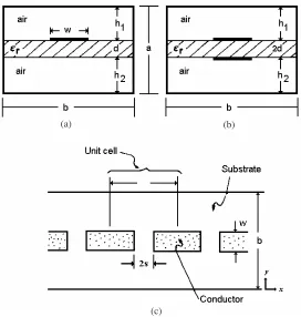
Figure 1. Cross-sectional views of suspended substrate line for periodic structures. (a) suspended stripline (h1 =h2), (b)
broadside-coupled suspended stripline, (c) periodic loaded pattern on the substrates.
2. ANALYSIS
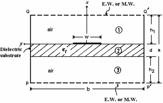
Figure 2. One half of the general suspended stripline with top and bottom walls as Electric or Magnetic walls for analysis.
The x-components of electric and magnetic fields can be driven by the solution of Helmholtz equation in the three homogenous regions (see Fig. 2).
Ex(1)= ∞
m=−∞
∞
n=1
Amn1cos[γmn1(x−h1)] cos(αny)e−jβmz (1.1)
Hx(1)= ∞
m=−∞
∞
n=0
Bmn1sin[γmn1(x−h1)] sin(αny)e−jβmz (1.2)
Ex(2)= ∞
m=−∞
∞
n=1
[Amn2sin(γmn2x)+Amn2cos(γmn2x)]cos(αny)e−jβmz (1.3)
Hx(2)= ∞
m=−∞
∞
n=0
[Bmn2cos(γmn2x)+Bmn 2sin(γmn2x)]sin(αny)e−jβmz (1.4)
Ex(3)= ∞
m=−∞
∞
n=1
Amn3cos[(γmn1(x+d+h2)] sin(αny)e−jβmz (1.5)
Hx(3)= ∞
m=−∞
∞
n=0
Bmn3cos[(γmn1(x+d+h2)] cos(αny)e−jβmz (1.6)
Fig. 2. The other parameters are:
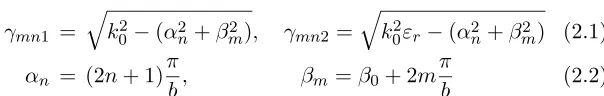
γmn1 =
k02−(α2
n+βm2), γmn2=
k20εr−(α2n+βm2) (2.1) αn = (2n+ 1)
π
b, βm =β0+ 2m
π
b (2.2)
β0in the dominant mode propagation constant andPis the periodicity,
they-components and z-components of the electric and the magnetic fields can be driven by using (1) in the Maxwell’s equations.
Ey(1)= ∞
m=−∞
∞
n=0
smn1sin[γmn1(x−h1)] sin(αny)e−jBmz (3.1)
Ey(2)= ∞
m=−∞
∞
n=0
[smn2cos(γmn2x)+Smn 2sin(γmn2x)]sin(αny)e−jβmz (3.2)
Ey(3)= ∞
m=−∞
∞
n=0
smn3sin[γmn1(x+d+h2)] sin(αny)e−jβmz (3.3)
Ez(1)= ∞
m=−∞
∞
n=1
Cmn1sin[γmn1(x−h1)] cos(αny)e−jβmz (3.4)
Ez(2)= ∞
m=−∞
∞
n=1
[Cmn2cos(γmn2x)+Cmn 2sin(γmn2x)]cos(αny)e−jβmz (3.5)
Ez(3)= ∞
m=−∞
∞
n=1
Cmn3sin[γmn1(x+d+h2)] cos(αny)e−jβmz (3.6)
Hy(1)= ∞
m=−∞
∞
n=1
Cmn1cos[γmn1(x−h1)] cos(αny)e−jβmz (3.7)
Hy(2)= ∞
m=−∞
∞
n=1
[Mmn2cos(γmn2x)+Mmn 2sin(γmn2x)]cos(αny)e−jβmz (3.8)
Hy(3)= ∞
m=−∞
∞
n=1
Cmn3sin[γmn1(x+d+h1)] cos(αny)e−jβmz (3.9)
Hz(1)= ∞
m=−∞
∞
n=0
Dmn1cos[γmn1(x−h2)] sin(αny)e−jβmz (3.10)
Hz(2)= ∞
m=−∞
∞
n=0
Hz(3)= ∞
m=−∞
∞
n=0
Cmn3cos[γmn1(x+d+h2)] sin(αny)e−jβmz (3.12)
In the above field expressions, there are eight unknown coefficients. Applying boundary conditions at x = 0 and x = −d, the unknown coefficients can be reduced to only Amn1 andBmn1.
3. DERIVATION OF CHARACTERISTIC EQUATION
By deriving the characteristic equation of the periodic structure, we need to express the unknown coefficients in terms of the transformed fields. We consider one unit cell of the periodic structure as shown in Fig. 1. Applying the orthogonal condition to unit cell, we obtain,
pb[αnCmnBmn1+βmSmnAmn1] = L2mn
pn(α2n+βm2)
(4.1)
pb[jβmCmnBmn1−jαnSmnAmn1] = L1mn
Qn(α2n+βm2)
(4.2)
where,
L2mn = p/2
−p/2
b/2
−b/2
Jzcos(αny)ejβmzdydz (4.3)
L1mn = p/2
−p/2
b/2
−b/2
Jysin(αny)ejβmzdydz (4.4)
pn =
1 forαn= 0
2 otherwise , Qn=
0 forαn= 0
2 otherwise (4.5)
Now by expressing the unknown coefficientsAmn1 andBmn1, in terms
of L2mn and L1mn we obtain, Amn1 =
1
pb [(βmPnL2mn−jαnQnL1mn)/(Smn)] (5.1) Bmn1 =
1
pb [(αnPnL2mn+jβmQnL1mn)/(Cmn)] (5.2) By consideringEy(1)andEz(1) atx= 0 and substitute the value ofAmn1
andBmn1, and applying the Galerkin’s method in transformed domain,
equations can be obtained. ∞
i=−∞
∞ j=1 cij ∞
m=−∞
∞
n=1
QnG11L(1i,jmn)L
(k,l) 1mn
+ ∞
i=−∞
∞ j=1 dij ∞
m=−∞
∞
n=1
PnG12L(2i,jmn)L
(k,l)
1mn= 0 (6.1) ∞
i=−∞
∞ j=1 cij ∞
m=−∞
∞
n=1
QnG21L(1i,jmn)L
(k,l) 2mn
+ ∞
i=−∞
∞ j=1 dij ∞
m=−∞
∞
n=1
PnG22L(2i,jmn)L
(k,l)
2mn= 0 (6.2) where,
k=−∞ to +∞; l= 1,2,3, . . . ,+∞ (6.3)
L(2k,lmn) = p/2
−p/2
b
0
e(yk,l)(y, z) cos(αny)e−jβmzdydz (7.1)
L(1k,lmn) = p/2
−p/2
b
0
e(zk,l)(y, z) sin(αny)e−jβmzdydz (7.2)
G11 = −sin (γmn1h1)
jβm2γmn1
Smn −
jwµ0αm2 Cmn
/αn2 +βm2 (8.1) G12 = −sin (γmn1h1)
αnβmγmn1
Smn −
wµ0αnβm Cmn
/α2n+βm2 (8.2)
G21 = −G12 (8.3)
G22 = −sin (γmn1h1)
jα2nγmn1
Smn −
jβm2wµ0
Cmn
4. FIELD DISTRIBUTION
Referring to the strip conductor pattern, shown in Fig. 2, the basis function strip current distribution in one unit cell of the periodic structure are,
ez(y, z) = 0 (9.1)
ey(y, z) = C01eay(y, z) +C−11eby(y, z) (9.2) eay(y, z) = eay(y)eay(z) =
1 +1 w
y−2s1
b−y
b−w
3
U(z)e−jβ0z,
s1 < y < s1+w (9.3)
eby(y, z) = eby(y)eby(z) =
1 +1 w
y−2s1
b−y
b−w
3
U(z)e−jβ−1z,
s1 < y < s1+w (9.4)
where:
eay(y) = eby(y) =
1 +1 w
y−2s1
b−y
b−w
3
=ey(y) (9.5)
eay(z) = U(z)e−jB0z (9.6)
eyb(z) = U(z)e−jβ−1z (9.7)
U(z) =
1 s <|z|< p/2
0 |z|< s
(9.8)
β−1 =
β0−
2π
p (9.9)
whereeay(y, z) andeby(y, z) are the basis functions corresponding to the dominant mode and the first special harmonic, respectively, and C01,
C−11 are unknown coefficients. 5. NUMERICAL RESULTS
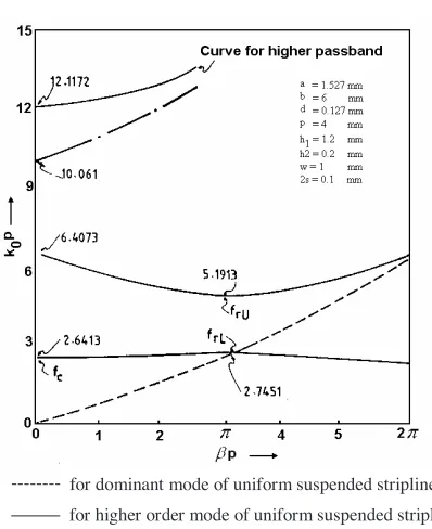
for dominant mode of uniform suspended stripline
for higher order mode of uniform suspended stripline
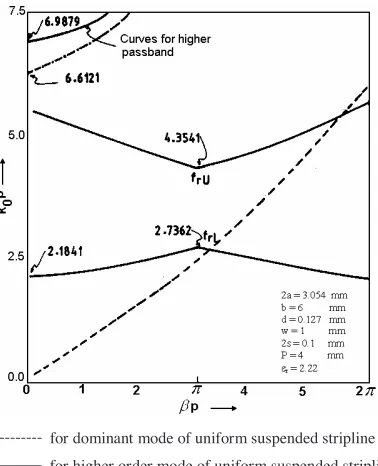
---Figure 3. k0−β0 diagram of suspended stripline periodically loaded
with series capacitive gaps.
Figure 3 illustrates a typicalk0−β0 diagram. The first passband
occurs in the frequency range whenk0P satisfy 2.4413< k0P <2.7451
and first stopband occurs in the range of 2.7451< k0P <5.1913 which
demonstrating very narrow passband and wide stopband the curve for the periodically loaded suspended stripline is above that for the uniform suspended stripline because of the capacitive reactance of the series gaps and the higher passband curves (k0 −β0) of the periodic
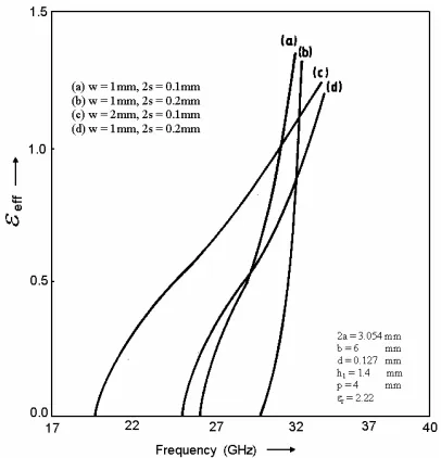
structure is above that of the uniform line for the higher order mode. Thus, the higher passbands and stopbands are not of much significance. Fig. 4 shows the variation in the stopbandwidth as a function of gap width 2s for two different value of stripwidth (w = 1 mm and w = 2 mm). The periodicity is held fixed at P = 4 mm. Thus as 2s is increased, the strip conductor lengthl decreases. Consequently, the resonant frequencyfrL increases. Fig. 4 also shows that an increase in 2s from 0.5 mm to 2 mm, frL increases where as the stopband width remains wide and fairly constant.
Figure 4. Effect of capacitive gap loading on the upper and lower frequency bounds (frU and frL) of the first stopband in suspended stripline periodically loaded with series capacitive gaps.
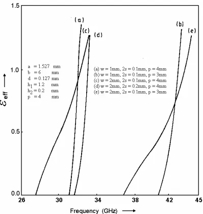
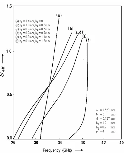
Figure 6. Dispersion of suspended stripline periodically loaded with series capacitive gaps for different combination ofh1 and h2.
Each curves in these figures corresponds to passband filter response. The frequencies corresponding to εeff = 0 give the cutoff frequencies and can be read from the horizontal axis. Also from Fig. 6, the curves marked a, b and dwhich are for 2s/w = 0.1 shows extremely narrow passband and curves cand ewhich are for lower value of 2s/w= 0.05 show wider passband, curve c is for P = 4 mm and curve e is for P = 3 mm. As expected, reducing the periodicity has the effect of shifting the passband to higher frequency.
In Fig. 5, with 2s/w = 0.05 and P = 4 mm we consider the effect of varying the air gap h1 (in which h2 = a−(d+h1), a and
dare fixed) on the dispersion characteristics, when in curve a,h2 = 0
(microstrip) and curve f when the strip conductor in extremely close to the topwall (h1 = 0.1 mm) very narrow passband results, where the
for dominant mode of uniform suspended stripline
for higher order mode of uniform suspended stripline
---Figure 7. k0−β0 diagram of broadside-coupled suspended stripline
periodically loaded with series capacitive gaps.
by 0.2 mm (i.e., h2 = 0.5 mm) has practically no effect on dispersion
characteristic.
The nature of k0 −β0 diagram in broadside-coupled suspended
stripline periodically loaded with series capacitive gaps with even mode excitation which is showing in Fig. 7, is similar to that of Fig. 3. The fact that the first passband starts from a finite value of k0P not zero,
is characteristic of the periodic pattern.
The effect of series gap loaded as shown in Fig. 8, we observe that the stopband width which is initially zero for 2s = 0 (uniform line) increases first with an increase in 2s and then decrease with fixing periodicity an increase in 2s, both frU and frL increase, and beyond a certain value of 2s, which frL continuous to increase, frU saturates thereby reducing the stopband width. For a sufficiently large value of 2swhen the adjacent strip conductors get increasing by decoupledfrL approaches the value offrU.
Figure 8. Effect of series gap loading on the upper and lower frequency bounds of the first stopband in broadside-coupled suspended stripline periodically loaded with series capacitive gaps.
that with wider strips, the width of first passband increase and that of first stopband decreases. Over the practical passband range, εeff has a value in the range of 0.0 to 1.5. Therefore this type of periodic configuration is no useful as a slow wave structure.
6. CONCLUSIONS
The suspended stripline with periodically loaded capacitive gaps is characterized by a lower cut-off frequency fc for the first passband (Fig. 3). The structure offers very narrow passband and wide stopband, particularly when the strip pattern is in close proximity to either the bottom or topwall. In Figs. 5 and 6the wider passband can be achieved by positioning strip conductor pattern at or close to the centre of the quide (curves b, c, d and e in Fig. 5 with εr = 2.22; the maximum value of εeff is less than about 1.5).
The characteristics of periodic broadside-coupled suspended stripline with the different periodic patterns are similar to the characteristic of the corresponding periodic structure in single conductor suspended stripline with symmetrically located substrate, in which the structure has a lower cut-off frequency,fc, narrow passband, wide stopband and εr in an approximate range 0 ≤ εeff ≤ 1.5 with patterns.
REFERENCES
1. Kiang, J. F., S. M. Ali, and J. A. Kong, “Propagation properties of striplines periodically with crossing strips,”IEEE Transactions on MTT, Vol. 37, 776–786, April 1989.
2. Koal, S. K., “Millimeter wave circuit techniques and technology for radar and wireless communication,” Proc. 4th International Conference on Millimeter Wave and for Infrared Sience and Technology, 206–209, Aug. 1996.
3. Packiaraj, D., M. Ramesh, and A. T. Kalghatgi, “Periodically loaded SSS coupled-line filter for second harmonic suppression,”
Microwave Journal, Vol. 49, No. 7, 106, July 2006.
6. Tounsi, M. L., R. Touhami, and A. Khodja, “Analysis of the mixed coupling in bilateral microwave circuits anisotropy for MICs and MMICs applications,”Progress In Electromagnetics Research, PIER 62, 281–315, 2006.
7. Jin, L., C. Ruan, and L. Chun, “Design E-plane bandpass filter based on EM-ANN mode,”Progress In Electromagnetics Research, PIER 20, No. 8, 1061–1069, 2006.
8. Jin, L. and C.-L. Ruan, “Neural network models for finline discontinuties,” International Journal of Infrared and Millimeter Waves, Vol. 25, No. 12, 1019–1027, 2004.
9. Casula, G. A., G. Mazzarella, and G. Montisci, “Effective analysis of a microstrip slot coupler,” Journal of Electromagnetic Waves and Applications, Vol. 18, No. 9, 1203, 2004
10. Mirshekar-Syahkal, D. and J. B. Davies, “Accurate analysis of coupled strip-finline structure for phase constant, characteristic impedance, dielectric and conductor losses,” IEEE Trans. on Microwave Theory and Tech., Vol. 30, No. 6, 906–910, June 1982. 11. Itoh, T. and A. S. Hebert, “A generalized spectral domain analysis for coupled suspended microstriplines with tuning septums,”