Estimation of the Number of Signal Sources in Presence
of Mutual Coupling
Ching S. Yu, Helio A. Muzamane, and Hsin-Chin Liu*
Abstract—The estimation of the direction of arrival (DOA) and the estimation of the number of signal sources are very important techniques in modern communications. The effect of mutual coupling can degrade the performance of the estimation algorithms. Mutual coupling compensation is used to mitigate this effect. However, errors remain when the compensation is carried out with such methods as minimum description length (MDL) to estimate the number of signal sources. This work presents a new method based on threshold decision to estimate the number of signal sources in presence of mutual coupling. The results of computer simulations demonstrate that the proposed method outperforms the MDL method.
1. INTRODUCTION
Smart antenna techniques have been studied for many decades. They are some of the most important techniques in support of the coming fifth-generation (5G) of mobile communication. Selected control algorithms with predefined criteria give adaptive antenna arrays the unique ability to alter the characteristics of their radiation patterns (nulls, side-lobe level, main beam direction and beam width) [1].
Direction of arrival (DOA) and number of signal sources estimations have many applications in wireless communication, radar, etc. This estimate can be performed using antenna arrays.
The performance of an adaptive antenna array is strongly influenced by the electromagnetic characteristics of antennas [2]. Therefore, to accurately evaluate the performance of practical antenna arrays, the electromagnetic influence of their elements must be considered. When two antennas are close to each other, some of the energy in one antenna is coupled to the other, causing an effect that is referred to as mutual coupling [1]. A mutual coupling matrix describes the effect of mutual coupling between antennas [2] and is constructed using the impedance matrix associated to the antenna elements of an array.
MUltiple SIgnal Classification (MUSIC) is the most well-known subspace-based method for estimating the DOA [1, 3, 4]. Eigenvalue Decomposition (EVD) is applied to the correlation matrix of an array output signal. The MUSIC algorithm exploits the orthogonality of the noise and signal subspaces to estimate the DOA.
The mutual coupling effect degrades the performance of array signal processing algorithms such as the DOA and algorithms used to estimate the number of signal sources. It is necessary to compensate for the effect of mutual coupling, as its presence can lead to a wrong estimate. To mitigate mutual coupling effect, mutual coupling compensation is used [5–8]. The calibration algorithm and maximum likelihood approach, have been used to calibrate the mutual coupling effect, but these methods require calibration sources of known location [9, 10]. The cost function has been used to mitigate the mutual
Received 29 June 2019, Accepted 26 August 2019, Scheduled 19 September 2019 * Corresponding author: Hsin-Chin Liu (hcliu@mail.ntust.edu.tw).
coupling effect [10, 11]. This method does not require a source of known location, but it uses an iterative process. The mutual coupling matrix has been used to modify the MUSIC pseudo-spectrum function to estimate the DOA [12, 13]. The inverse of mutual coupling matrix is used to compensate for mutual coupling [14].
To estimate the number of signal sources, the Akaike information criteria (AIC) and the minimum description length (MDL) have been proposed [15, 16]. These methods usually assume the noise to be Additive White Gaussian Noise (AWGN) and that the signals are uncorrelated. However, when an array receives a line-of-sight (LOS) signal and its multi-path components, their correlation leads to detection errors. To obtain the spatially smoothed correlation matrix, forward backward spatial smoothing techniques (FBSS) were developed [17]. Different methods to determine the number of signal sources were studied [18, 19].
In this paper we propose a new method based on a threshold decision rule. The threshold value is related to the noise power (after mutual coupling compensation) and the mutual coupling compensation term, which is then, used for the estimation of the number of signal sources. Among the aforementioned algorithms, the MDL is one of the well-known algorithms. We hence compare our proposed method with the MDL algorithm in this work.
Throughout this paper, we use the following notations: C to denote the set of complex numbers,
R to denote the set of real numbers, E[.] to define the expectation operator, tr(.) to define the trace operator,1y to denote anM dimensional vector containing ones, (.)m to represent a signal with mutual coupling, (.)mcto represent a signal after mutual coupling compensation and (.)cto represent the mutual coupling compensation component.
This paper is organized as follows: Section 2 gives the background; Section 3 describes the proposed method; Section 4 presents simulation results; and Section 5 draws conclusions.
2. BACKGROUND
2.1. System Model with Mutual Coupling
Balanis and Ioannides [1] and Gross [4] mathematically described the model of an ideal array output signal. Let’s consider an ideal array withM sensors (antennas) receivingN uncorrelated signals. Each received signal is a narrowband plane wave from far-field emitters. The ideal array output vector
x(t)∈CM×1 is given as
x(t) =
N
i=1
a(ϕi)βisi(t) +n(t)
x(t) =Aβs(t) +n(t)
(1)
where a(ϕi) ∈ CM×1 is the steering vector corresponding to the angle ϕi of the ith incoming signal; diag{βi} = β ∈ CN×N is the diagonal matrix that contains the channel gain of the ith signal path; [s1(t), . . . , sN(t)]T =s(t)∈CN×1 is the incoming signal vector; and n(t) ∈CM×1 is the Gaussian noise vector containing elements with zero mean and variance σ2. We combine β and s(t) as α(t) = βs(t). The steering matrix A∈CM×N is given by
A= [a(ϕ1),a(ϕ2), . . . ,a(ϕN)] (2) The correlation matrix of the ideal array output signal Rx∈CM×M is given by
Rx =Ex(t)xH(t) =ARαAH +σ2I
=Rs+Rn
(3)
whereIis anM×M identity matrix, andRα ∈CN×N is the correlation matrix of the incoming signals
The output signal vector with mutual coupling xm(t) ∈ CM×1 includes the matrix that contains the mutual coupling elements and is given by
xm(t) =CAα(t) +n(t) (5) where C ∈ CM×M is the mutual coupling matrix that is constructed using the impedance matrix associated to the antenna elements of an array and is defined as [2]
C=
Z
ZL +I −1
(6)
in whichZandZL are the mutual impedance matrix and the load impedance in each antenna element, respectively. The correlation matrix of the array output signal with mutual coupling Rmx ∈ CM×M
becomes
Rmx =E
xm(t) (xm(t))H
=CARαAHCH +σ2I
(7)
2.2. Estimation of the Number of Signal Sources
One of the most known subspace methods for DOA estimation is MUSIC. To perform MUSIC algorithm, we need to estimate the number of the received signals in an antenna array first, so that the dimensions of the signal and noise subspaces can be determined accordingly.
The MUSIC algorithm is based on the orthogonality of the noise and signal subspaces. Considering that Rα is non-singular and that the columns of A are independent, from Eq. (3) it follows that the rank of ARαAH is N. After the EVD is carried out, the matrixARαAH hasN positive eigenvalues and M-N zero eigenvalues. We denote the eigenvalue by λj and the corresponding eigenvector by ej
forj∈ {1, . . . , N, N+ 1, . . . , M}. Ignoring the presence of noise we have
Rx =Rs=
N
m=1
λmemeHm+ M
m=N+1
0emeHm (8)
Since the noise is present, i.e.,σ2 >0,Rx is a full rank matrix and hasM positive and real eigenvalues. The N largest eigenvalues correspond to the signal and the M-N smallest eigenvalues correspond to the noise variance. The correlation matrix of the ideal output signal, after EVD is given by
Rx=
N
m=1
λmemeHm+
M
m=N+1 σ2e
meHm (9)
For a better understanding on the concept, we build vectors with all eigenvalues asλs+σ21M =λx∈ M×1, in whichλ
s ∈ M×1 is the vector containing the eigenvalues ofRsand σ21M composes the noise
variance vector. The eigenvalues are sorted in descending order as follows
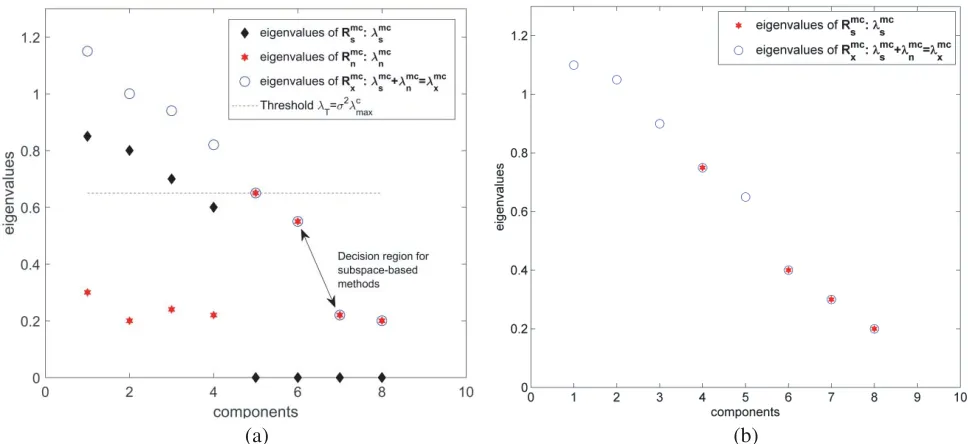
λ1 > . . . > λN λN+1=. . .=λM =σ2 (10) Figure 1(a) graphically shows the structure of the eigenvalues in the case where no coupling is considered. From the subspace methods, the number of signal sources is estimated as the number of the eigenvalues that are greater than the noise variance.
The MUSIC pseudo-spectrum has been defined in [1, 3]. Although it has high resolution, this subspace method is applicable when the signals are uncorrelated.
The application of information theoretic criteria for model selection by Rissanen (the MDL method) has been described in [15] and [16]. The number of signal sources is determined as the value for which the MDL criterion is minimized.
Given a set of datax(tl), l∈ {1, . . . , P} and considering the covariance matrix of the output signal in Eq. (3), with the source signal covariance matrix of rank k, the problem is formulated as how to select the best model (the one that best fits with the signal model) from the following models
R(xk)=
k
j=1
(a) (b)
Figure 1. (a) Graphical representation of eigenvalues without mutual coupling effect. (b) Graphical representation of eigenvalues after mutual coupling compensation.
in whichλj and ej are the eigenvalue and the eigenvector ofR(xk), respectively. The parameter vector to be estimated is denoted as Θ(k) and is given as
Θ(k)=λi, . . . , λk, σ2,eH1 , . . . ,eHk (12) Considering that the observations are statistically independent complex Gaussian vectors with zero mean, it follows that their joint probability density function (PDF) is given by
fx(t1), . . . ,x(tP)|Θ(k)
=
P
j=1 1 πMdetR(k)
x
exp
−x(tj)H
R(k)x
−1
x(tj)
(13)
Note that the distribution of the signal x(tj) is conditioned to the noise distribution. Therefore, if the noise is no longer white Gaussian, the above expression no longer holds.
The log-likelihood function, omitting terms that do not depend on Θ(k), becomes
LΘ(k)
=−Plog det
R(xk)
−tr
R(xk)
−1
ˆ R
(14)
whereRˆ is the sample covariance matrix and is given as
ˆ R= 1
P
P
j=1
x(tj)xH(tj) (15)
Maximizing the expression in Eq. (14), we get the maximum likelihood estimates of the vector Θ(k). The estimates are as in [19] and given as
ˆ
λj = ˆlj, j= 1, . . . , k (16a)
ˆ
σ = 1
M −k
M
j=k+1 ˆ
lj (16b)
ˆ
where ˆl1 ≥ . . . ≥ ˆlM and ˆu1, . . . ,ˆuM are the sample eigenvalues and eigenvectors of Rˆ, respectively. Substituting Eq. (16) in Eq. (14) we obtain
LΘˆ(k)= log
⎛ ⎜ ⎜ ⎜ ⎜ ⎜ ⎝ M
j=k+1 ˆ lM1−k
j
1 M −k
M
j=k+1 ˆ lj ⎞ ⎟ ⎟ ⎟ ⎟ ⎟ ⎠
P(M−k)
(17)
Based on the MDL principle, the selection model is the one that minimizes the following expression
MDL(k) =−L
ˆ Θ(k)
+ 1
2ηlog(P) (18)
in which η is the number of free adjusted parameters in Θ. Substituting Eq. (17) in Eq. (18) and pluggingη as in [19], we have
MDL(k) =−log
⎛ ⎜ ⎜ ⎜ ⎜ ⎜ ⎝ M
j=k+1 ˆ lM1−k
j
1 M−k
M
j=k+1 ˆlj
⎞ ⎟ ⎟ ⎟ ⎟ ⎟ ⎠
P(M−k)
+ k
2(2M−k) log(P) (19)
The number of signal sources N is determined as the argument kthat minimizes Eq. (19).
The MDL method is more feasible to detect the number of signal sources as it is not limited to uncorrelated signals. However, MDL depends on the number of snapshots P (the good performance is reached as the number of snapshots increases) and when a more realistic model that includes the mutual coupling effect is considered, the MDL and the other subspace methods fail. This is because after mutual coupling compensation, the noise is no longer white Gaussian (AWGN), violating an essential assumption on which these methods depend. The MDL is a well-known algorithm for the estimation of the number of received signals. Consequently, we compare our proposed method with the MDL algorithm in the simulations. The following section presents a novel solution to this problem.
3. THE PROPOSED METHOD
The effect of mutual coupling can be mitigated by mutual coupling compensation. Multiplying the received signal by the inverse of the mutual coupling matrix in Eq. (7) [14] yields
Rmcx =C−1Rmx C−1H
=ARαAH+σ2C−1 C−1H
=Rmcs +Rmcn
(20)
Note that, after mutual coupling compensation,Rmcs =RsandRmcn =σ2C−1(C−1)H are the covariance matrices. The noise term is multiplied by the mutual coupling compensation matrix C−1(C−1)H invalidating the white noise assumption, as can be seen from the second term on the right-hand side in Eq. (20). Applying the EVD to Eq. (20) we get
Rmcx =
N
m=1
λmcm emcm (emcm )H+
M
m=N+1
λmcm emcm (emcm )H (21)
We build vectors with all eigenvalues as λmcs +λmcn = λxmc ∈ M×1, in which λmcs = λs is the vector containing the eigenvalues ofRs (after mutual coupling compensation), andλmcn ∈ M×1 is the vector containing the noise eigenvalues multiplied by the mutual coupling compensation matrix, respectively. The eigenvalues are arranged as in the following descending order
λmc
Because of the contamination of the noise term, the eigenvalues in Eq. (22) cannot be separated in the same way as in Eq. (10). From subspace methods, the number of signal sources would then be determined based on the white noise assumption, which is not valid to Eq. (22).
From the eigenvalues in Eq. (22) and graphically represented in Fig. 1(b), our goal is to find a threshold value so that we can still separate those eigenvalues that belong to the signal.
Mutual coupling can be measured from the elements of an array. The mutual coupling matrix has full rank and by applying the EVD to the mutual coupling compensation term we get
C−1 C−1H =
M
m=1
λcmecm(ecm)H (23)
We defineλT as the threshold value, which is given by
λT =σ2λcmax (24)
whereλcmaxrepresents the maximum eigenvalue of the matrixC−1(C−1)H. At high signal-to-noise ratio (SNR), no eigenvalue that belongs to the contaminated noise term might be estimated to be higher than the product of the noise variance and the maximum eigenvalue of the mutual coupling compensation matrix. ThereforeλT can be used as the threshold value to separate the eigenvalues related to the signal from the eigenvalues related to the noise. The number of signal sources is estimated as the number of eigenvalues λmci ,i∈ {1, . . . , M}that will be greater than the threshold.
Let’s consider a case as in Fig. 2(a), where the number of signal sources is N = 4. Because the largest gap (the reference for these methods) among the eigenvalues comes after λ6, according to the subspace methods as in Eq. (10), the number of signal sources is estimated to be N = 6, which is not true. Although the MDL method does not determine the number of signals merely by observing the eigenvalues, it is still based on the signal and noise subspaces. Considering mutual coupling compensation, these subspaces are no longer separable, making the estimation with MDL method to be a challenge and leading to error as well. However, the proposed method estimates the correct number as it takes the maximum eigenvalue λcmax together with the noise variance to make the threshold.
The problem that is identified in this paper is solved, and the simulation results in the following
(a) (b)
section show the reduction in estimation errors. The proposed method can be implemented in the following steps:
Step 1: Calculate the correlation matrix of the array output signal with mutual coupling effect as in Equation (7);
Step 2: Perform mutual coupling compensation as in Equation (20) to mitigate the effect of mutual coupling;
Step 3: Perform EVD as in Equations (21) and (23);
Step 4: Estimate the number of incoming signals by using the proposed method, which is based on the threshold detection rule and built as in Equation (24).
Although our method performs well compared with those presented in this paper, as proven graphically and through simulations, it can present errors to detect the number of signal sources in a low SNR regime. Considering the case in Fig. 2(b), defining the threshold value, the proposed algorithm would also give a wrong estimate because in this case, the threshold lies on the componentλ4.
4. SIMULATION RESULTS
We consider 16 dipole antennas that form a uniform linear array (ULA). The array impedance value quantifies the interaction between the antenna elements and has been simulated using Ansys R, the High Frequency Structure Simulator (HFSS) from www.ansys.com. Fig. 3(a) shows the results. The horizontal and vertical axes of the figure contain the values that indicate the antenna element ports and from them, the impedance magnitude can be read. The impedance matrix that was used to construct the mutual coupling matrix in Eq. (6) is used in the simulations. In order to approach a more realistic model, we extended our simulations to the case where the incoming signals are highly correlated. Spatial smoothing guarantees that the signal correlation matrix is of full rank. The FBSS correlation matrix of an array output signal is as defined in [17] and is applied in our simulations.
The parameters for the simulations are set as in Table 1. From the table, U is for the angle that is uniformly distributed at a specified range. The performances of the proposed method with mutual coupling compensation (calibration), MDL with mutual coupling compensation (calibration) and MDL
(a) (b)
Table 1. Parameter values.
Parameter (unit) Value
Pulse width,TP W 50
Pulse repetition interval 1
Number of samples 3780
Number of signals,N 4
Channel gain, β1,β2,β3,β4 |β1|
= 1,|βi| ∼U(0.5,1)|, i= 2,3,4 ∠βi ∼U(0,2π), i= 1,2,3,4
Channel delay,δ12,δ13,δ14 δ12= 6,δ13= 9,δ14= 13
DOA (degrees) θi = 90
◦,i= 1,2,3,4;
ϕi ∼U(0◦,180◦), i= 1,2,3,4
Sensor type Dipole
Array type Uniform Linear Array
Carrier frequency, fc (GHz) 3
Interspacing of sensors (cm) 5.0
Monte Carlo trials, Q 5000
without mutual coupling compensation (no calibration) are presented. The latter two methods are denoted as MDL (CAL), and MDL (NCA), respectively.
Furthermore, we compare the performance of the proposed method in three cases as shown in Fig. 3(b). From the figure, we can see that the estimation accuracy slightly, degrades as the number of antennas decrement. However, the estimation accuracy still outperforms the MDL in high SNR regime when the mutual coupling effect is taken into account.
With mutual coupling, the proposed method is more accurate to determine the number of signal sources than the MDL method. Fig. 4(a) plots the root mean square error (RMSE) as function of SNR for all methods. It reveals that the proposed method performs almost as well as MDL (NCA) but outperforms it for SNR greater than 14 dB. This result demonstrates the feasibility of using the
(c) (d)
(e) (f)
Figure 4. Performance of the proposed method versus the MDL method evaluated from root mean square error (RMSE) and Bias for (a) and (b) M = 16 antenna elements, (c) and (d)M = 12 and (e) and (f)M = 8.
proposed method.
Figures 4(a), (b), (c), (d), (e), and (f) clearly show how the MDL (CAL) detection errors are more significant than those of the other methods, because after the mutual coupling compensation the noise in each element is no longer white Gaussian. The MDL (NCA) yields an excessive number of signal sources at certain values of SNR but the proposed method yields the true number. Fig. 4(b) plots the estimation bias against the SNR in which a clear biased estimate of the MDL (CAL) and of the MDL (NCA) for the SNR values greater than 14 dB is shown.
M = 12 and the performance of the proposed method is still more accurate than MDL method. When M = 8, Figs. 4(e) and (f), the RMSE of the proposed method is not good as of the MDL, but it still outperforms the MDL one from the values of SNR greater than 19 dB, see Fig. 4(e). Form Fig. 4(f), can be seen that the bias of the proposed method is consistently improved than the one of the MDL method.
5. CONCLUSION
This work presents a new method to estimate the number of signal sources in the presence of mutual coupling effect. The subspace methods such as MUSIC algorithm lead to detection errors when the incoming signals are highly correlated but methods such as Rissanen MDL applicable to both cases where the signals are uncorrelated or highly correlated. When an array is built with a more realistic approach (considering the effect of mutual coupling), the mutual coupling compensation causes such methods to fail. The proposed method is based on the threshold decision, in which the threshold value is built from the components of mutual coupling compensation matrix and the noise variance. Our method improves upon MDL (CAL) and MDL (NCA). In our simulations the model is extended to the case where the signals are even correlated. The proposed method outperforms the MDL method (in a more realistic environment) and so enables the number of signal sources to be estimated.
REFERENCES
1. Balanis, C. A. and P. I. Ioannides, Introduction to Smart Antennas, Morgan & Claypool, 2007. 2. Gupta, I. J. and A. A. Ksienski, “Effect of mutual coupling on the performance of adaptive arrays,”
IEEE Transactions on Antenna and Propagation, Vol. 31, 785–791, September 1983.
3. Schmidt, R., “Multiple emitter — Location and signal — Parameter estimation,” IEEE Transactions on Antennas and Propagation, Vol. 34, 276–480, 1986.
4. Gross, F., Smart Antennas with MATLAB, McGraw Hill Professional, 2015.
5. Basikolo, T., K. Ichige, and H. Arai, “A novel mutual coupling compensation method for under-determined direction of arrival estimation in nested sparse circular arrays,” IEEE Transactions on Antennas and Propagation, Vol. 66, 909–917, 2018.
6. Ye, Z. and C. Liu, “2-D DOA estimation in the presence of mutual coupling,”IEEE Transactions on Antennas and Propagation, Vol. 56, 3150–3158, 2008.
7. Ye, Z. and C. Liu, “A methodology for mutual coupling estimation and compensation in antennas,”
IEEE Transactions on Antennas and Propagation, Vol. 61, 1119–1131, 1994.
8. Ki, D.-W. and N. Sangwook, “Mutual coupling compensation in receive-mode antenna array based on characteristic mode analysis,”IEEE Transaction on Antennas and Propagation, Vol. 66, 7434– 7438, December 2018.
9. See, C. M. S., “Sensor array calibration in the presence of mutual coupling and unknown sensor gains and phases,”Electronics Letters, Vol. 30, 373–374, 2012.
10. Samson, B. and C. Ng, “Sensor-array calibration using a maximum-likelihood approach,” IEEE Transactions on Antennas and Propagation, Vol. 44, 827–835, 1996.
11. Friedlander, B. and A. Weiss, “Direction finding in the presence of mutual coupling,” IEEE Transactions on Antennas and Propagation, Vol. 39, 273–284, 1991.
12. Sellone, F. and A. Serra, “A novel online mutual coupling compensation algorithm for uniform and linear arrays,”IEEE Transactions on Signal Processing, Vol. 55, 560–573, 2007.
13. Svantesson, T., “Modeling and estimation of mutual coupling in a uniform linear array of dipoles,”
1999 IEEE International Conference on Acoustics, Speech, and Signal Processing, Vol. 5, 2961– 2964, 1999.
14. Huang, Z., C. Balanis, and C. Birtcher, “Mutual coupling compensation in UCAs: Simulations and experiment,” IEEE Transaction on Antennas and Propagation, Vol. 54, 3082–3086, 2006.
16. Wax, M. and I. Ziskind, “Detection of the number of coherent signals by the MDL principle,”IEEE Transactions on Acoustics, Speech, and Signal Processing, Vol. 37, 1190–1196, August 1989. 17. Pillai, S. and B. Kwon, “Fonvard/Backward spatial smoothing techniques for coherent signal
identification,” IEEE Transactions on Acoustic, Speech, and Signal Processing, Vol. 37, 8–15, January 1989.
18. Claudio, E. and R. Parisi, “Space time MUSIC: Consistent signal subspace estimation for wideband sensor arrays,”IEEE Transaction on Signal Processing, Vol. 66, 6118–6128, 2018.