Multi-Objective Optimization of Wireless Power Transfer Systems with Magnetically Coupled Resonators and Nonlinear Loads

Multi-Objective Optimization of Wireless Power Transfer Systems

with Magnetically Coupled Resonators and Nonlinear Loads

Johan Winges1, *, Thomas Rylander1, Carl Petersson2, Christian Ekman2, Lars-˚Ake Johansson2, and Tomas McKelvey1

Abstract—We present an optimization procedure for wireless power transfer (WPT) applications and test it numerically for a WPT system design with four resonant circuits that are magnetically coupled by coaxial coils in air, where the magnetic field problem is represented by a fully populated inductance matrix that includes all magnetic interactions that occur between the coils. The magnetically coupled resonators are fed by a square-wave voltage generator and loaded by a rectifier followed by a smoothing filter and a battery. We compute Pareto fronts associated with a multi-objective optimization problem that contrasts: 1) the system efficiency; and 2) the power delivered to the battery. The optimization problem is constrained in terms of: 1) the physical construction of the system and its components; 2) the root-mean-square values of the currents and voltages in the circuit; and 3) bounds on the overtones of the currents in the coils in order assure that the WPT system mainly generates magnetic fields at the operating frequency. We present optimized results for transfer distances from 0.8 to 1.6 times the largest coil radius with a maximum power transfer from 4 kW to 9 kW at 85 kHz, which is achieved at an efficiency larger than 90%.

1. INTRODUCTION

Wireless transmission of electrical energy from a source to a device has received increased attention in recent years [1]. The current interest of wireless power transfer (WPT) is mainly focused on devices with batteries that require frequent charging such as mobile phones, laptops, medical implants, vehicles and trains. For short-range applications, contactless power transfer systems [2] are relatively mature and used in many commercial applications today. Naturally, it is desirable to extend this technology to situations that feature a significantly larger distance between the source and the device, which often are referred to as mid-range applications. One promising technique for mid-range applications such as wireless charging of electric vehicles is inductive power transfer systems with magnetically coupled resonators [3, 4].

For a very challenging problem in terms of power transfer distance, Kurset al.[5] transfer 60 W at an efficiency of about 40% ford/rmax = 8, wherermax is the radius of the two resonant coils that they

use, anddis the distance between the source coil and the device coil. Kesler [6] presents an analysis of this system in terms of circuit theory, where it is assumed that: 1) the source and the device circuits are resonant at the oscillation frequency of the generator; and 2) the generator resistance and load resistance can be chosen in a favorable manner. Given this situation, the efficiency is η = U2/(1 +√1 +U2₎2_,

where U =k12 √

Q1Q2 for the coupling coefficient k12 and the quality factors Qi of the source and the

device. For applications that require higher power delivered to the load, it is desirable to increase the efficiency in order to avoid excessive heating of the WPT system. Should highQ_i be maintained for the

Received 15 November 2018, Accepted 11 January 2019, Scheduled 17 January 2019

* Corresponding author: Johan Winges ([email protected]).

source and the device, high efficiency can be accomplished for systems with lower d/rmax, since such

geometrical configurations make it possible to increasek12substantially. A number of options have been

presented ford/rmax1 and, typically, these systems target the wireless charging of vehicles [3, 7]. For

d/rmax= 0.5, Bosshard et al. [8] demonstrate an optimized WPT system capable of transferring up to

5 kW at an efficiency of 96%.

The WPT systems [3, 5–8] exploit Nr = 2 resonant circuits, where one is located on the primary

side of the system (i.e., the source) and the other on the secondary side of the system (i.e., the device). Kiani and Ghovanloo [9] demonstrate a system withNr resonant circuits that are magnetically coupled

and, for the range 2 < d/rmax < 4, they achieve a higher efficiency for Nr = 3 and 4 as compared

to Nr = 2, which may be attributed to the additional degrees of freedoms associated with the extra

resonant circuits. However, the analysis presented by Kiani and Ghovanloo [9] requires that: 1) all the resonant circuits are resonant at the oscillating frequency of the generator; and 2) each coil only couples magnetically to its immediate neighbors, which yields a tridiagonal inductance matrix that simplifies the analysis. These prerequisites make it possible to arrive at analytic expressions for the efficiency by means of coupled mode theory [5] or reflected load theory [10]. Based on these principles, Huiet al.[11] demonstrate a relay arrangement for WPT with a larger number of magnetically coupled resonant circuits, where 2 ≤ Nr ≤ 8. Additional analytic derivations for multi-coil relay WPT systems can be

found in [12, 13]. Frequency splitting [11, 14] has been identified as a design problem for WPT systems with multiple resonant circuits that share the same resonant frequency. If frequency splitting occurs, the power delivered to the load may become significantly reduced, unless for example the generator frequency is increased or decreased as a means of compensation. This may be problematic for applications where regulations require that the WPT is carried out at a fixed frequency.

In this article, we present a constrained multi-objective optimization procedure for nonlinear WPT systems that contrasts the two objectives: 1) the system efficiency; and 2) the power delivered to the battery. The WPT system is modeled by a set of magnetically coupled resonators fed by a square-wave voltage source (that models the power inverter) and loaded by a rectifier followed by a smoothing filter and a simple battery model, which yields a nonlinear WPT system-model. Our optimization problem is subjected to practically realistic constraints on: 1) the physical construction of the system and its components; 2) the root-mean-square values of the currents and voltages in the circuit; and 3) bounds on current overtones in the coils. The constraints are determined by the application and they are not only important from a practical perspective, but they also have a significant impact on the optimized designs. In relation to the optimization objectives, we note that Hui et al. [11] argue that it is important to maximize the output power for large d/rmax and that it is typically easier to achieve

high efficiency. We find that our multi-objective optimization approach is useful since it exposes the performance limitations of the WPT system in regards to both power transfer and efficiency, where the system design is subject to the constraints for the application at hand. This is unusual in the open literature, where an exception is the work by Bosshard et al. [8, 15] forNr = 2.

We employ genetic algorithms [16, 17] to solve this multi-objective optimization problem for the time-periodic state that follows after the transient stage when the WPT system is energized. In the context of the optimization problem, the resonance frequencies of the magnetically coupled resonators are allowed to be independent of each other and the oscillation frequency of the generator. This is in stark contrast to many analytical results found in the literature such as [9, 18, 19], where the resonance frequencies of all resonators are forced to be equal to the generator frequency. Given a resistive load connected directly to the power inverter, we derive expressions for the optimal load resistance subject to constraints on the generator’s current and voltage. Our optimization procedure retrieves this optimal load resistance approximately for the WPT systems considered in this article, and to the best of our knowledge, this type of results is not available in the open literature.

We test our optimization procedure on a family of WPT systems with 0.8≤d/rmax ≤1.6, which

can be based on rather standard off-the-shelf components in order to achieve a modest over-all cost for the WPT system, which in turn implies a number of rather severe constraints on the currents and voltages for the various components and subsystems of the WPT system. Moreover, we constrain the current overtones in the coils to ensure that the WPT system mainly generates magnetic fields in the frequency band 81–90 kHz in accordance to the SAE standard [20]. In order to simultaneously fulfill these objectives and constraints, we useNr= 4 magnetically coupled resonance circuits. To facilitate for

large scale optimization, we use a simple coil model with four circular coaxial coils in free space, which can be accurately described with Biot-Savart’s law [21]. Naturally, a realistic WPT system intended for wireless charging of vehicles requires magnetic materials to guide the magnetic fields in the proximity of the metal chassis of the vehicle. However, the coil system in free space yields reasonable results for the magnetic coupling coefficient as compared to geometrically similar systems that use magnetic materials, where the magnetic coupling coefficient is the most important circuit parameter derived from the field problem. Also, it should be emphasized that our optimization procedure works equally well for WPT systems that use magnetic materials that require additional computational cost associated with the more involved field problem. The coil and circuit model employed in this article have been experimentally verified in [22], where we presented a (non-optimal) four coil WPT system capable of transferring 3.4 kW at 91% system efficiency to a resistive load. The circuit model was also experimentally verified in [23], where we show that a safe magnetic field strength is possible to realize at the edge of a small vehicle for a 3 kW WPT system using magnetic materials. In this article, we present simulated results with optimal power transfer and efficiency for a range of transfer distances to a battery load.

2. SYSTEM MODEL

Figure 1 shows a schematic diagram of the WPT system that consists of: 1) a power inverter; 2) a set of magnetically coupled resonators; and 3) a rectifier with a filter connected to the load. The power inverter is fed by a constant voltage source.

source

P ower inverter

Rectifier and filter

load Wireless p ower transfer system

Magnetically coupled resonators

Figure 1. Schematic diagram for the wireless power transfer system.

2.1. Power Inverter

The power inverter is modeled by a voltage source uG(t) in series with a resistance RG as shown in

Figure 2(a), where the square-wave voltage is given by

uG(t) =U0sgn [cos(ωpt)]. (1)

Here, the angular frequency is ωp = 2πfp, and the corresponding period is Tp = 1/fp for a power

inverter that operates at the frequencyfp. The power inverter is constrained by the maximum voltage

amplitudeU₀max such thatU0≤U0max.

2.2. Magnetically Coupled Resonators

RG + uG iG A1 A2 P ower inverter

R1 L11 i1 C1 + u1 A1 A2 R2 L22 i2 C2 + u2 R3 L33 i3 C3 + u3 R4 L44 i4 C4 + u4 iB B1 B2 + uB

Primary side Secondary side

(b) (a)

Figure 2. Circuit diagram for: (a) the power inverter; and (b) the magnetically coupled resonators.

to the power inverter and, in our case with N = 4, the dashed box contains the components associated with the primary side. The secondary side is indicated by the dashed box with the terminals B1–B2,

which are connected to a load that is characterized by iB =iB(uB) with uB =u4. Thus, we have the

circuit model

L∂i

∂t =u−Ri+uG, (2)

C∂u

∂t =−i−iB(uB), (3)

where the state of the circuit is described by the current vector i = [i1, i2, i3, i4]T and the voltage

vector u = [u1, u2, u3, u4]T. Further, we have the excitation voltage vector uG = [uG,0,0,0]T and the

load current vector iB(uB) = [0,0,0, iB(uB)]T. The diagonal matrices C = diag(C1, C2, C3, C4) and

R= diag(RG+R1, R2, R3, R4) represent the capacitors and resistors, respectively. Finally, the self and

mutual inductances are represented by the inductance matrix L, which is a fully populated matrix to account for all magnetic coupling within and between the primary and secondary sides.

2.3. Load Models

The simplest load is a resistor RL connected directly to the terminals B1-B2. Then, iB(uB) = GLuB

with the conductance GL = 1/RL and we have iB = Gu in Eq. (3), where G = diag(0,0,0,1/RL).

Consequently, Eqs. (2)–(3) can be solved as a linear circuit for a time-harmonic excitation.

For situations that involve charging of a battery, we consider a full-wave rectifying circuit that consists of four diodes with a smoothing filter connected to a simple model of a battery as shown in Figure 3. The battery is modeled by an internal resistance RB and an electromotive force EB. For the

diodes shown in Figure 3, we use a piecewise linear current-voltage characteristic

iD=iD(uD) =

0 ifuD≤uFB,

(uD−uFB)/RD ifuD> uFB,

(4)

whereuFB is the forward-bias voltage-drop andRDis the forward resistance.

D1

D2

D3

D4 B1 B2

LSF 1

C₁SF

LSF 2

C₂SF

+

uout

RB

iout

εB

3. METHOD

3.1. Time-Domain Analysis and Modelling

The circuit model in Eqs. (2)–(3) together with the generator and load model yields a time-domain representation of the system that can be expressed as a state-space model, where the currents through inductors and the voltages over capacitors are collected in a single state vector y(t). The state-space model can be written as a system of coupled ordinary differential equations on the form

˙

y(t) =A(y(t))y(t) +B(y(t))x(t), (5) where the matrices A and B depend on the state vector y(t), i.e., if the diodes in the circuit are conducting or not. Sources are collected in the forcing vector x(t).

For a time interval of unchanged conduction states for the diodes, we have a linear circuit (given our piecewise linear model for the diodes) and the matricesA and B are constant. Then, the solution of Eq. (5) for t≥t_i is

y(t) =F(t)y(t_i) +

_t

ti

F(t−τ)Bx(τ)dτ, (6)

where y(t_i) is the initial state, and we have introduced the matrix exponential F(t) = eA(t−ti)_{. We}

construct an explicit time-stepping scheme based on the state-space model of Eq. (5) and its explicit solution of Eq. (6), where we assume that x(t) is constant for t≥ t_i. Given a finite time-step Δt, we update the solution according to Eq. (6) fromt_itot_i+1 =ti+ Δt. As a default value, we use Δt=Tp/N

withN = 512, and if needed for convergence, we increase N by a factor 2k for a positive integer kand restart the simulation. At every time step, the conduction conditions for the diodes are evaluated, and A,B and xare changed accordingly. The time stepping is stopped after the transients have vanished, and the voltages and currents are time-periodic with a relative tolerance of 10−3.

For the time-periodic currents and voltages, we are interested in the input and output power and the system efficiency

¯

pin=pin(t)=

1 Tp

_t0+Tp

t0

uin(t)iin(t)dt, (7)

¯

pout =pout(t)=

1 Tp

_t0+Tp

t0

uout(t)iout(t)dt, (8)

η= pout(t)

pin(t)

, (9)

where · denotes the time average for one period fromt0 tot0+Tp, and it is assumed that the system

is time-periodic for t ≥ t0. Here, uin(t) = uG(t) and iin(t) = iG(t), where uG and iG are defined in

Figure 2(a). The output voltage and current are defined in Figure 3.

3.1.1. Time-Harmonic Representation

A signal s(t) (i.e., a current or voltage) that is time-periodic can be decomposed in a Fourier series

ncnexp[j2πnt/Tp]. For the fundamental mode of s(t), we use phasor notation and introduce the

complex amplitude ˆs = 2c1, which corresponds to the part of the signal that is useful for the power

transfer. In addition, we denote the effective value of the phasor by ˜s = ˆs/√2. In order to assure that the WPT system mainly produces magnetic fields at the operational frequency, we find it useful to extract the undesired overtones as

δs(t) =s(t)−Re

ˆ sexp

j2πt

Tp

, (10)

in order to impose constraints onδs(t) when necessary.

We note that in practice, the equivalent load impedanceZA connected to the terminals A1-A2 of

the power inverter is required to have ∠ZA ≥0◦ to achieve inductive operation of the power inverter

and zero-voltage-switching [15, 24].

3.2. Optimization

We optimize the WPT system in terms of the two objectives given by Eqs. (8) and (9) that depend on the time-periodic circuit state y(t). It should be noted that these two objectives are conflicting [11] in the sense that their extrema do not, in general, coincide. The objective functions can be organized in a vector g = [g1, g2] according to g1(p) = ¯pout(p;q) and g2(p) =η(p;q). Here, p describes the design of

the system in terms of component values and other design parameters that are subject to optimization, and q describes design parameters that are not subject to optimization such as: 1) different load conditions, and 2) varying power transfer distanced.

Both the objective functions ing(p) are constructed to be used in the context of a maximization problem, and we have the multi-objective optimization problem

max

p [g1(p), g2(p)]

s.t.y(t) = time-periodic circuit solution described by p, pL ≤p≤pU,

U0 =U0∗(p),

(11)

which involves explicit constraints (pL,pU) on the component values directly or their geometrical design

parameters. Given a specific system design described byp, the maximum amplitudeU₀∗(p) that can be used by the power inverter is determined by an inner optimization problem

U₀∗= max

U0 U0

s.t.y(t) = time-periodic circuit solution described by p, c(y(t))≤cU,

U0 ≤U0max.

(12)

Here, the constraints c on the state vector y(t) are expressed in terms of the root-mean-square (rms) value of currents and voltages in the circuit, which clearly depend on U0. The rms value is defined as · rms=

(·)2_.

We solve the optimization problem in Eq. (11) by a genetic algorithm (GA) [17, 25] and the inner optimization problem in Eq. (12) that features the nonlinear constraints by bisection [26]. Given the resonant nature of the WPT system, the optimization problem features many local extrema, and thus, it is useful to exploit GAs. In addition, GAs can handle optimization problems with mixed integer and real-valued parameters, which is required for the WPT system that we consider in this article.

In this article, we do not include the constraint ∠ZA ≥ 0◦ that is required to ensure inductive

operation of the power inverter. This choice is based on the following experiences: 1) the optimal solutions typically yield ∠ZA0◦; 2) enforcing this constraint severely reduces the convergence speed

of the genetic optimization algorithm employed; and 3) A small negative angle∠ZA>−10◦can typically

be compensated for without significant loss of performance by increasing theC1 capacitance value. In

an effort to assure that inductive operation is realizable, any solutions with ∠ZA ≤ −10◦ have been

removed after optimization.

4. RESULTS

Below, we present results for two cases: 1) a linear circuit with time-harmonic excitation and an approximately equivalent load resistanceRL; and 2) a nonlinear circuit with the time-periodic excitation

in Eq. (1) and the battery load shown in Figure 3. Further, we demonstrate a simple C1 compensation

4.1. Test Problem

In the following subsections we present the choice of component models and constraints that describe the test problem considered in this article, where our choices are motivated by wireless charging systems for electric vehicles. We stress that the coil and circuit model employed in this article have been experimentally verified in [22], where we presented a non-optimal four coil WPT system capable of transferring 3.4 kW at 91% system efficiency to a resistive load at the transfer distance d/rmax = 0.4.

Here, we consider the optimization of a similar WPT system design where larger transfer distances and power levels are feasible.

4.1.1. Power Inverter

The power inverter operates at the frequencyfp = 85 kHz with a maximum voltage amplitude ofU0max

= 450 V. Thus, we have the phasor ˆumax_G = (4/π)U₀max for the fundamental mode and its effective value is ˜umax_G = (2√2/π)U₀max = 405 V. In addition, we constrain the current for the power inverter by

iG(t)rms≤I0max= 30 A. The generator resistance RG is 0.25 Ω.

Here, our choice of frequency is motivated by the SAE standard J2954 [20], which is intended to establish a common frequency band for wireless charging of light-duty vehicles. The choice of maximum voltage, current and generator resistance are motivated by a conservative design of a power inverter based on four transistors of type 45N65M5 from STMicroelectronics.

4.1.2. Magnetically Coupled Resonators

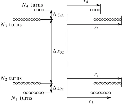
We consider an axisymmetric system of four coils in free space such that each coil consists of a single layer of windings that can be described by: 1) coordinate z_m along the axis of symmetry; 2) outer coil-radiusr_m; and 3) number of turnsN_m. The geometry is shown in Figure 4, where Δz_mn=z_m−z_n. The primary and secondary sides are separated by an air gap of distance Δz32, which is subject to the

constraint Δz32 ≥ d. Thus, we can compute all the entries Lmn of the inductance matrix based on

Biot-Savart’s law [21], where the self and mutual inductances may be expressed in terms of elliptical integrals [27] as we approximate each turn in a coil by a closed circular loop. Further, Δz21 and Δz43

are required to be larger than 17 mm to assure that there is axial space between the different coils for a fixture. These geometrical design criteria allow for a relatively simple coil construction, where the coil wire can be wound around a thin cable reel similarly as shown in [22].

In an attempt to illustrate the relation between these coils in free space and the corresponding coils of an actual WPT system for the charging of electric vehicles, we consider the coils as viewed from the circuit based on their inductance matrix representation. The magnetic coupling coefficients of the coil

N1 t urns N2t urns N3t urns

N4t urns

r1 r2 r3 r4

Δz21 Δz32 Δz43

system do not change significantly as magnetic-material plates are placed, in close vicinity, below coil 1 and above coil 4. (Obviously, the magnetic materials significantly change the magnetic fields that surround the charging region between the coils.) The absolute inductances of a system with magnetic materials may be reduced (and the free space values recovered) if an appropriate number of turns are removed from each coil. Thus, a coil arrangement with magnetic materials can be constructed in such a manner that it yields an inductance matrixL_μ that approximates the corresponding inductance matrix Lof the coils in free space shown in Figure 4. For remaining deviations between the inductance matrices, possible performance reductions may be compensated for by changing the capacitances as demonstrated in [22]. Thus, an optimized WPT system based on coils in free space may be modified and implemented with magnetic materials and, thus, adopted for charging of electric vehicles. However, such a system has additional losses that stem from the magnetic materials and eddy current losses.

In a broader sense, the coils in free space provide fast analysis combined with an inductance matrix that incorporate the most important dependencies on the geometrical parameters that describe the coils. Given an optimized design presented in this article, the inductance matrix (viewed from the circuit) may be realized in terms of the electric-vehicle application that requires coils with magnetic materials, which in itself can be considered as yet another a design problem. If the performance of such a two-step procedure is not satisfying, its final design can be used as a starting point for a more refined optimization procedure that is based on a detailed field model of the WPT system together with the electric vehicle, where both magnetic and conducting materials are incorporated.

Given that Litz wire is used for the coils, the resistance of the m-th coil can be approximated as R_m =l_m/(σA), whereσ is the bulk conductivity of the Litz-wire conductor, A the cross section of the wire, and l_m the wire length of them-th coil. Based on the Litz-wire used in [22, 23], the diameter of the copper conductor in the Litz-wire is 4.9 mm, and we set the distance between turns in the radial direction to 5 mm. The specified Litz-wire diameter allows for a current of 60 A without excessive heating. Also, a resistance R0 = 0.1 Ω is added to the coil wire resistance. Here, R0 represents an

estimate of additional losses for the resonant circuits found from measurements in [22], where examples of such loss contributions are contact resistances in the circuit and the dielectric losses in the capacitors. It is assumed that it is possible to realize the capacitances C_m for a range of values such that the frequency f_m = 1/(2π√L_mmC_m) for resonant circuit m = 1, . . . ,4 can be selected between 50 kHz to 200 kHz. Here,f_m can be interpreted as the resonance frequency of them-th resonator ifthe magnetic coupling to all the other resonators is discarded. In the context of optimization, we find it attractive to work with f_m = 1/(2π√L_mmC_m), which replaces the capacitance C_m as a design parameter given a known value for L_mm. Consequently, this is nothing but a change of variables for the optimization procedure, and it is further discussed in Section 4.1.5. Obviously, the system of magnetically coupled resonators has resonant frequencies that differ from our design parametersf_m used during optimization. In practice, the capacitancesC_m could be implemented by means of constructing a capacitor bank with, e.g., polypropylene film capacitors organized in a Cartesian grid with Np parallel columns of Ns

identical discrete capacitors connected in series. Here, Ns determines the voltage constraint and Np

the current constraint for the capacitor bank, in combination with the choice of discrete capacitors. For ease of construction, we also limit the total number of capacitors by including a constraint on the voltage-current product for each capacitor bank.

4.1.3. Rectifier, Smoothing Filter and Battery

The diodes in the rectifier are characterized in terms of the forward-bias voltage-dropuFB = 0.92 V and

the forward resistance RD = 0.11 Ω, where these values are motivated by the diode C4D05120A from

Cree. The smoothing filter components are given by LSF₁ = 30µH, C₁SF = 20µF, LSF₂ = 2.2µH and C₂SF = 10µF. The battery is modelled by an internal resistanceRB = 0.25 Ω and an electromotive force EB in the range of from 310 V to 390 V, which approximately represent a multi-cell lithium-ion battery

for vehicles for a range of different state-of-charge (SOC).

4.1.4. Circuit Model Validation

uses considerably more elaborate models for the transistors in the power inverter and the diodes in the rectifier. We find that we have less than 2% deviation between the currents and voltages in our model and the more elaborate LTspice IV model for the time-periodic state. The time-periodic model have also been experimentally verified for the WPT systems presented in [22, 23], where the deviations are typically less than 10% between simulation and experiment.

4.1.5. Optimization Parameters

Table 1 shows all the parameters subject to optimization and, therefore, incorporated in the parameter vector p. It should be noted that the component values L_mn and R_m are computed from the coils’ geometry, where the number of turnsN_m is only allowed to take integer values. Further, we introduce the resonance frequency ω_m = 1/√C_mL_mm associated with the m-th resonator. We optimize with respect tof_m=ω_m/(2π), and then, the corresponding capacitance is determined asC_m = 1/(ω_m2L_mm). This choice is based on our experience that the optimization algorithm converges in fewer iterations if we usef_m instead ofC_m. The constraints for pL and pU are also listed in Table 1.

Table 1. Parameters subject to optimization in the multi-objective optimization problem (11) with minimum and maximum bounds given an application specific design box.

Component Quantity unit min max

Coil r_m m 0.1 0.25

N_m - 1 15

Δz21 m 0.017 0.1

Δz32 m d d+ 0.1

Δz43 m 0.017 0.1

Resonance frequency f_m kHz 50 200

4.1.6. Constraints

Given this test problem, the constraints are listed in Table 2. These constraints are motivated by component limitations imposed by practical considerations and to avoid excessive heating and voltage breakdown. The constraint on the overtones δi(t)rms can be used to ensure that the WPT

system mainly generates magnetic fields in the frequency band 81–90 kHz in accordance to the SAE standard [20].

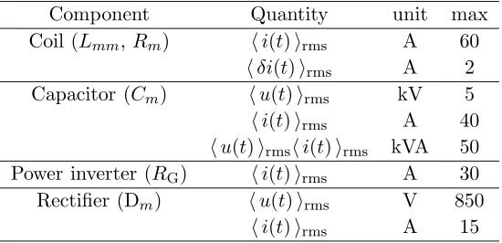
Table 2. Constraints on currents and voltages for the components listed within the parentheses that are deemed appropriate for the intended power level in the WPT application.

Component Quantity unit max Coil (L_mm,R_m) i(t)rms A 60

δi(t)rms A 2

Capacitor (C_m) u(t)rms kV 5

i(t)rms A 40

u(t)rmsi(t)rms kVA 50

Power inverter (RG) i(t)rms A 30

Rectifier (D_m) u(t)rms V 850

4.2. Linear Circuit with Time-Harmonic Excitation

According to the analysis in [8, 29], the nonlinear load in Figure 3 may be approximated as an equivalent load resistance RL = (πEB)2/(8 ¯pout). This makes it possible to construct a linear circuit

that approximates the WPT system at its fundamental time-harmonic component of frequency fp,

and the results may be compared with the corresponding nonlinear system. Thus, we consider the four magnetically coupled resonators (shown in Figure 2(b)) fed by a time-harmonic voltage at the frequency ω =ωp and loaded by a resistance RL connected to the terminals B1-B2, which gives a linear circuit

with time-harmonic excitation that we can treat in the frequency domain. The magnetically coupled resonators are subject to optimization, where we consider the range of air gap distances dbetween the primary and secondary sides given by 20 cm≤d≤40 cm.

Figure 5 shows Pareto fronts that contrast system efficiency η and power ¯pout delivered to the

resistanceRL= 35 Ω for relative distances in the interval 0.8≤d/rmax≤1.6. We note thatη decreases

monotonically as ¯poutis increased, which confirms that the two objectives are conflicting. For sufficiently

low values of ¯pout, none of the constraints in Table 2 are active. As ¯pout is increased, one or several

constraints become active, and the system efficiency deteriorates at a higher pace. In Figure 5, it is primarily the constraints u(t)rmsi(t)rms for m = 1,2,3 that become active. For each of the fixed

value ofd/rmax, we achieve a similar Pareto front as the optimization problem is solved for a different

load resistanceRL, where we have tested the range 15 Ω≤RL≤55 Ω.

2 4 6 8 10 12

0.88 0.9 0.92 0.94 0.96 0.98 1

0.8 0.9 1.0 1.1 1.2 1.3 1.4 1.5 1.6

Figure 5. Pareto fronts that contrast efficiency and power delivered to the load resistance RL = 35 Ω

for 0.8 ≤ d/rmax ≤1.6, where rmax = 25 cm. The magnetically coupled resonators are fed by a

time-harmonic voltage and optimized subject to the constraints in Table 2.

Table 3 shows the optimized results p and derived circuit quantities for four designs located on the Pareto front shown in Figure 5 with d/rmax= 1.2. For the optimized designs shown in Table 3, we

note that: 1) f_m =fp for all resonant circuit in contrast to the work by Kiani and Ghovanloo [9] that

requiref_m =fpfor allm; 2)f1andf4are reduced as the Pareto front is traversed fromp∗R1top∗R4; and

3) N1 and N4 are both reduced slightly. In addition, rm =rmax for all four coils andNm =Nmax for

m= 2 and 3. We stress that the Pareto front exposes the important trade-off between power transfer and efficiency and that an appropriate Pareto-optimal solution should be selected depending on the application specifications. For example, designp∗_R1 (3.6 kW power transfer at 97% efficiency) could be appropriate for an efficient charging station suitable for overnight use while design p∗_R4 could be used for a faster charging solution with the considerably higher maximum power transfer of 7.5 kW at 93% efficiency. Naturally, if even higher power levels are to be realized, the voltage and current constraints must be increased correspondingly or a shorter transfer distance selected.

Table 3. Design parameters p and derived circuit quantities for four optima on the Pareto front in Figure 5 ford/rmax= 1.2.

Optimump∗_R1 Optimump∗_R2 Optimump∗_R3 Optimump∗_R4 Param. p_out= 3.66 kW, η= 0.97 p_out= 5.08 kW, η= 0.97 p_out= 6.73 kW, η= 0.95 p_out= 7.54 kW, η= 0.93

m 1 2 3 4 1 2 3 4 1 2 3 4 1 2 3 4

Nm 15 15 15 4 15 15 15 4 14 15 15 3 10 15 15 3

rm[cm] 25 25 25 25 25 25 25 25 25 25 24.9 25 25 25 25 25

zm[cm] 0 1.76 31.8 35.3 0 1.77 31.8 35.2 0 2.34 32.4 34.3 0 3.53 33.5 35.8

fm[kHz] 131 103 87.8 195 122 107 87.9 191 113 110 94.8 137 96.7 111 95.9 126

Lmm[μH] 157 157 157 19 157 157 157 19 142 157 157 11.5 86.3 157 157 11.5

Cm[nF] 9.44 15.3 20.9 35.3 10.9 14.1 20.9 36.5 14 13.3 18 118 31.4 13.1 17.5 139

Rm[mΩ] 118 118 118 106 118 118 118 106 117 118 118 104 113 118 118 104

k1m[%] - 80.1 8.0 6.0 - 80.0 7.9 6.0 - 74.3 7.6 6.1 - 62.0 7.0 5.6

k2m[%] - - 8.8 6.5 - - 8.8 6.6 - - 8.8 7.0 - - 8.8 6.8

k3m[%] - - - 53.7 - - - 54.1 - - - 60.6 - - - 58.5

Figure 2(a), where ZA corresponds to the magnetically coupled resonators and the load RL. Figure 6

shows ZA = RA+jXA as the Pareto front is traversed for d/rmax = 1.2 and d/rmax = 0.8. The

curves are discontinued at the point where a higher power transfer cannot be achieved without violating the constraints. We consider the reactance to be close to zero, i.e., XA 0, for most parts of the

Pareto front. Thus, we find that the generator is effectively loaded with a resistance RA. Given this

situation, a simple model consists of the power inverter shown in Figure 2(a) connected directly to a resistive loadRA. Then, the power delivered to the load is ¯pout = ˜u2_GRA/(RG+RA)2 u˜2_G/RA, which

is shown as ZA = RA = ˜u2_G/p¯out by the dash-dotted curve in Figure 6. Furthermore, Appendix A

presents an analysis of this circuit with constraints on the generator voltage and current such that ˜

uG ≤ u˜maxG and ˜ıG ≤ ˜ımaxG , where ˜umaxG = 405 V and ˜ımaxG = 30 A for the power inverter considered

here. For maximum power transfer toRAin this simple circuit, we arrive at an optimal load resistance

2 4 6 8 10 12

0 10 20 30 40 50 60 70 80

Figure 6. ImpedanceZAas a function of power delivered to the load resistance as the Pareto front in

Figure 5 is traversed for: (◦) d/rmax = 1.2; and () d/rmax = 0.8. The input impedance is computed

at the terminals A1-A2 in Figure 2(b). The real part of the impedance is described by the solid curve

R_A∗ = ˜umax_G /˜ımax_G −RG = 13.25 Ω, since ˜umax_G /˜ımax_G ≥2RG. For d/rmax = 0.8, it is interesting to note

thatRAapproachesR∗Afor large values of ¯pout, which indicate that the power inverter can be optimally

loaded and that primarily the generator constraints limit the maximum power transfer.

4.3. Nonlinear Circuit with Time-Periodic Excitation

Next, we consider the four magnetically coupled resonators (shown in Figure 2(b)) fed by a square-wave voltage and loaded by a rectifier followed by a smoothing filter and a battery (shown in Figure 3). The magnetically coupled resonators are subject to optimization, where we consider the range of air gap distancesdbetween the primary and secondary sides given by 20 cm≤d≤40 cm.

Figure 7 shows Pareto fronts that contrastη and ¯pout for the magnetically coupled resonators for

0.8≤d/rmax≤1.6 and EB = 380 V. For each of the fixed value ofd/rmax, we achieve a similar Pareto

front as the optimization problem is solved for a different electromotive force EB, where we have tested

the range 310 V≤ EB≤390 V. For most of the Pareto fronts, it is noted that the constraintδi(t)rmsis

active for the currents throughL11and L44, which is reasonable since the current throughL11is driven

by the power inverter that is rich in overtones, and L44 is close to the rectifier that may excite strong

overtones. Also, we note that similarly as for the linear circuit, the constraints u(t)rmsi(t)rms for

m= 1, 2, 3 become active as ¯pout is increased, and thus, they limit the power transfer.

2 3 4 5 6 7 8 9 10

0.9 0.91 0.92 0.93 0.94 0.95 0.96 0.97

0.8 0.9 1.0 1.1 1.2 1.3 1.4 1.5 1.6

Figure 7. Pareto fronts that contrast efficiency and power delivered to the battery EB = 380 V for

0.8≤d/rmax≤1.6, wherermax= 25 cm. The magnetically coupled resonators are fed by a square-wave

voltage and optimized subject to the constraints in Table 2.

Table 4 shows the design parameters p and derived circuit quantities for four Pareto-optimal designs, which are indicated in Figure 7 ford/rmax = 1.2. Interestingly, r4 is clearly smaller than rmax

for the nonlinear circuit, which was not the case for the linear circuit. Also, the distance Δz43 is about

5 cm, which is more than twice the distance found for the linear circuit. These choices combined yield a rather low coupling coefficient 0.39 ≤ k34 ≤0.47 between the resonant circuit m = 3 and 4 for the

nonlinear circuit. Furthermore, Figure 8(a) showsL_mm as the Pareto front (d/rmax= 1.2) is traversed.

Here, we notice in particular thatL44is rather small in comparison to the other inductances. Similarly,

Figure 8(b) shows ω_m/ωp. Typically, we notice rather gradual changes in ωm as the Pareto front is

traversed and that ω_m > ωp for all resonators m. It is interesting to note that the values for Lmm

are rather similar to the time-harmonic case, which nevertheless features a somewhat similar load at ωp. However, the values for ω4/ωp are significantly smaller and, as a consequence, C4 is now larger for

the nonlinear circuit. One possible interpretation of this result is that a larger C4 yields a rather low

impedance in parallel with the inductance L44, which in turn makes the capacitor C4 act as a sink for

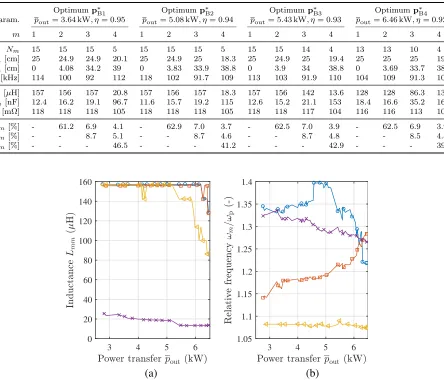
Table 4. Design parameters p and derived circuit quantities for four optima on the Pareto front in Figure 7 ford/rmax= 1.2.

Optimump∗_B1 Optimump∗_B2 Optimump∗_B3 Optimump∗_B4 Param. p_out= 3.64 kW, η= 0.95 p_out= 5.08 kW, η= 0.94 p_out= 5.43 kW, η= 0.93 p_out= 6.46 kW, η= 0.92

m 1 2 3 4 1 2 3 4 1 2 3 4 1 2 3 4

Nm 15 15 15 5 15 15 15 5 15 15 14 4 13 13 10 4

rm[cm] 25 24.9 24.9 20.1 25 24.9 25 18.3 25 24.9 25 19.4 25 25 25 19.5

zm[cm] 0 4.08 34.2 39 0 3.83 33.9 38.8 0 3.9 34 38.8 0 3.69 33.7 38.7

fm[kHz] 114 100 92 112 118 102 91.7 109 113 103 91.9 110 104 109 91.3 108

Lmm[μH] 157 156 157 20.8 157 156 157 18.3 157 156 142 13.6 128 128 86.3 13.7

Cm[nF] 12.4 16.2 19.1 96.7 11.6 15.7 19.2 115 12.6 15.2 21.1 153 18.4 16.6 35.2 160

Rm[mΩ] 118 118 118 105 118 118 118 105 118 118 117 104 116 116 113 104

k1m[%] - 61.2 6.9 4.1 - 62.9 7.0 3.7 - 62.5 7.0 3.9 - 62.5 6.9 3.9

k2m[%] - - 8.7 5.1 - - 8.7 4.6 - - 8.7 4.8 - - 8.5 4.8

k3m[%] - - - 46.5 - - - 41.2 - - - 42.9 - - - 39.0

3 4 5 6

0 20 40 60 80 100 120 140 160

3 4 5 6

1.05 1.1 1.15 1.2 1.25 1.3 1.35 1.4

(b) (a)

Figure 8. Optimized circuit parameters as the Pareto front in Figure 7 is traversed for d/rmax= 1.2:

(a) Inductance L_mm. (b) Resonance frequency ω_m/ωp that also determines the capacitance Cm =

1/(ω2_mL_mm). The glyphs correspond to the different resonators as indexed in Figure 2(b): (◦) m = 1; () m= 2; () m= 3; and (×) m= 4.

also find that the corresponding load impedanceZB =RB+jXB at the terminals B1-B2 in Figure 2(b)

is inductive for the battery load, where the resistive and reactive parts are comparable. Consequently, the approximate equivalent load resistance [8, 29] given by RL = (πEB)2/(8 ¯pout) must be generalized

to an appropriately selected equivalent load impedanceZL, should optimization of a WPT system with

battery load based on a linear circuit model be accurate.

Next, we compute the equivalent load impedanceZA for the fundamental frequencyωp. Figure 9

shows ZA as we traverse the Pareto front in Figure 7 for d/rmax = 1.2 and d/rmax = 0.8. Similarly

as for the time-harmonic case, we note that ZA is primarily resistive, although larger deviations from

XA= 0 are present, which is particularly true ford/rmax = 1.2. Although a clear decrease in efficiency

is noted between the different transfer distances, we observe no significant difference inZAin the range

4 kW ≤p¯out ≤6 kW in Figure 9. Consequently, it appears important to effectively load the generator

by a resistive load ZA RA = ˜u2G/p¯out to achieve optimal power transfer, but it is not a sufficient

2 3 4 5 6 7 8 9 10 0

10 20 30 40 50 60 70 80

Figure 9. ImpedanceZAas a function of power delivered to the battery as the Pareto front in Figure 7

is traversed for: (◦) d/rmax = 1.2; and () d/rmax = 0.8. The impedances are computed for the

fundamental frequency as described in Section 3.1.1. The real part of the impedance is described by the solid curve and the imaginary part by the dashed curve. The black dash-dotted curve shows the load impedanceZA=RA= ˜u2G/p¯out for a simple generator and load model.

4.4. Compensation Using C1 for Inductive Operation

During operation of the power inverter, we require that its load is inductive, which implies that the equivalent load impedance ZA=RA+jXA has a positive reactance XA. If the equivalent load of the

power inverter is capacitive withXA<0, a rather simple counter measure is to decrease the resonance

frequency frequency f1 = 1/(2π √

L11C1) of the first resonant circuit by increasing the capacitance C1.

We stress that such a compensation typically does not decrease the system performance for the optima presented here, and if necessary, more elaborate compensation schemes that vary all four capacitors can be exploited [22].

As an example, we consider the optimized system p∗_B4 during start-up, where the power inverter voltage U0 is increased up to U0∗ as determined by the optimization problem in Eq. (12). The solid

curves in Figure 10(a) presents ZA as U0 is increased from 50 V to 380 V. Here, the reactance XA is

negative for U0 < 320 V and, thus, compensation is necessary for inductive operation of the power

inverter. The dashed curves in Figure 10(a) show ZA for a simple and ad-hoc compensation scheme,

where C1 is changed such that f1 is increased linearly from 0.85f1∗ at U0 = 50 V to f1∗ at U0 = 380 V

given the optimized frequencyf₁∗ = 104 kHz. It is clear that this simple measure yields XA>0 for all

U0.

Figure 10(b) shows the system performance by solid curves for the uncompensated case and by the dashed curves using the C1 compensation scheme. In contrast with the uncompensated case, it

is possible to achieve high efficiency also for the range 100 V < U0 < 170 V using the compensation

scheme. In practice, a control system could change C1 to achieve sufficiently good performance and, if

necessary, the capacitances of the other resonators could also be adjusted as demonstrated in [22].

4.5. Characteristic Charging Behavior for Optimized System

100 200 300 0

5 10 15 20 25 30

-20 -15 -10 -5 0 5 10 15

100 200 300 0

0.2 0.4 0.6 0.8 1

0 1 2 3 4 5 6 7

(b)

(a)

Figure 10. (a) Impedance ZA in terms of resistance RA (×) and reactance XA (◦) versus U0. (b)

Efficiency (×) and power transfer to the battery (◦) versus U0. Both figures show the results for the

transfer distance d/rmax = 1.2 using the design parameters for optimum p∗B4 by solid curves. The

dashed curves show the corresponding results using a simple compensation scheme for the optimump∗_B4 where C1 is changed such that f1 is linearly increased from 0.85f1∗ at U0 = 50 V to f1∗ at U0 = 380 V.

The horizontal dashed-dotted line in (a) shows XA= 0.

and various active circuits are used to help achieve a safe and reliable charging according to a specific charging cycle.

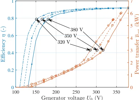
As an example, we consider the optimized design p∗_B4 and its performance characteristics in the context of constant-current and constant-voltage charging, where the design p∗_B4 is optimized for

EB = EBmax = 380 V. Figure 11 shows the system efficiency and power delivered to the battery as

a function of the voltage amplitude U0 ≤ U0∗, where results for EB = 320 V, 350 V and 380 V are

shown. We note that the efficiency and power transfer characteristics are rather similar for the different electromotive forces of the battery, where these deal with a range 0.85E_Bmax<EB≤ E_Bmax. Consequently,

the optimized system p∗_B4 can follow an increasing EB given an increasing amplitude U0 =U0∗ for the

100 150 200 250 300 350 0

0.2 0.4 0.6 0.8 1

0 1 2 3 4 5 6 7

Figure 11. System efficiency (×) and power transfer to the battery (◦) as a function of the generator voltage U0 for the transfer distanced/rmax= 1.2 using the design parameters for optimump∗_B4 at three

power inverter, and this solution may work rather well for constant-current charging of a lithium-ion battery pack, should the WPT system be equipped with a suitable control system and active circuitry. Next, we note that the constant-voltage charging is described approximately by the caseEB=EBmax in

Figure 11, where the output voltage of the smoothing filter is rather constant, and the current through the rectifier (and into the battery) is approximately proportional to ¯pout. Again, a suitable control

system and active circuitry would be necessary. In practice, the power inverter’s duty cycle could be changed instead of the peak voltage U0.

5. CONCLUSIONS

We have presented an optimization framework that yields competitive designs for a WPT system that features real-world challenges: 1) a nonlinear load with rectifier, smoothing filter and battery; 2) optimization with respect to multiple objectives that contrast system efficiency and power delivered to the battery; 3) realistic design-constraints that express component limitations, restrictions on size and current overtones in the coils; and 4) a fully populated inductance matrix that gives a complete port-to-port representation based on the magnetic field problem for the full set of coils of the WPT system. We find our optimization approach attractive in the sense that it exposes the important performance trade-offs necessary to consider in many WPT applications. In particular, we note that the current and voltage constraints limit the maximum realizable power transfer in a complicated manner.

For a family of test problems motivated by wireless charging systems for vehicles, we present Pareto fronts that contrast the system efficiency versus the power delivered to the battery for a WPT system with four magnetically coupled resonators. The Pareto fronts are computed for a range of distances 0.8≤d/rmax≤1.6, wherermax= 25 cm is the maximum radius of the coils, anddis the power transfer

distance.

For the separate resonators indexed by m, we note that our optimized results feature resonance frequencies ω_m = 1/√L_mmC_m that vary as the Pareto front is traversed and, in addition, that these resonance frequencies tend to take values that do not coincide with the excitation frequencyωp of the

generator. In contrast, many analytical results found in the literature assume that ω_m =ωp for all m,

and thus, we conclude that such choices indeed yield relatively simple analytical expressions that are easy to work with but may very well also be sub-optimal for a constrained WPT system.

The maximum realizable power transfer is found to primarily depend on the voltage and current constraints for the circuit for a given value of d/rmax, and we find that the four magnetically coupled

resonators and load behave approximately as an equivalent resistance connected to the power inverter after optimization. However, we find that the corresponding construction for the rectifier, smoothing filter and battery requires an equivalent impedance, where the inductive reactance is comparable to the resistance. Furthermore, we consider a battery load with its electromotive forceEB in the range 310 V ≤ EB ≤390 V and conclude that an optimized WPT system can achieve similar performance for this

entire range, should it be optimized for the largest value of EB. Thus, the optimized WPT systems

could be used to supply power to a battery load with varying state-of-charge by controlling the voltage of the power inverter.

ACKNOWLEDGMENT

This work was funded by the Swedish Energy Agency in the project “S¨aker induktiv energi¨overf¨oring f¨or elfordon – Safe Wireless Energy (SAWE)”, which has the project number 38577-1. The computations were performed on resources at Chalmers Center for Computational Science and Engineering (C3SE) provided by the Swedish National Infrastructure for Computing (SNIC).

APPENDIX A. CONSTRAINED GENERATOR WITH RESISTIVE LOAD

To analyze the effects of voltage and current constraints on the generator, we consider the simple model where the generator is modelled as a voltage source ˜uG in series with an internal resistanceRG,

and a load resistance RA is connected to its terminals. For a well-functioning WPT system with low

on the output of the power-inverter’s terminals is approximately real. We let the effective value of the generator voltage and current be constrained by

˜

uG≤u˜maxG and ˜ıG ≤˜ımaxG (A1)

where ˜umax_G and ˜ımax_G are constants derived from the physical components that are used in the power inverter. According to Ohm’s law ˜uG = Rtot˜ıG, the generator voltage is bounded by ˜uG ≤ u˜maxG =

min(˜umax_G , Rtot˜ımaxG ), where Rtot =RG+RA. Thus, the generator’s input power ¯pmaxin and the output

power ¯pmax_out delivered to the load are bounded by ¯

pin≤p¯maxin = min (˜umaxG )2/Rtot, Rtot(˜ımaxG )2

, (A2)

¯

pout ≤p¯maxout = min (˜umaxG )2RA/R2tot, RA(˜ımaxG )2

, (A3)

which yields the efficiencyη = ¯pout/p¯in=RA/Rtot.

According to Eq. (A1), the maximum possible generator power is ¯pmax_G = ˜umax_G ˜ımax_G , for which we define the efficiencies

χG =

¯ pmax_in ¯ pmax

G

= min (ξ/Rtot, Rtot/ξ), (A4)

χA=

¯ pmax_out ¯

pmax_G = min RAξ/R

2

tot, RA/ξ

, (A5)

where ξ = ˜umax_G /˜ımax_G . For ξ = Rtot, we find that both the constraints in Eq. (A1) are active

simultaneously which yields χG = 1 and χA = RA/Rtot = η. For ξ = Rtot, only one of the two

constraints in Eq. (A1) is active, and the generator cannot be fully utilized.

Next, we search for the maximum power transfer toRA by maximizingχA= min(χA,1, χA,2) with

respect toRA. We find two cases: 1) ifξ≤2RG, thenχAmax=ξ/(4RG) atRA=RGfrom the maximum

of χA,1; and 2) if ξ ≥2RG, then χmaxA = 1−RG/ξ at RA=ξ−RG from the intersection between χA,1

and χA,2. Our analysis leads to the rather interesting conclusion that the maximum power transfer

occurs at the effective load resistance R∗_A = ˜umax_G /˜ımax_G −RG for ˜umaxG /˜ımaxG ≥ 2RG. We emphasize

that R∗_A does not coincide with the conventional impedance matching condition R∗_A=RG, which only

applies to ˜umax_G /˜ımax_G ≤2RG.

REFERENCES

1. Jawad, A. M., R. Nordin, S. K. Gharghan, H. M. Jawad, and M. Ismail, “Opportunities and challenges for near-field wireless power transfer: A review,” Energies, Vol. 10, No. 7, 2017.

2. Kazmierkowski, M. P. and A. J. Moradewicz, “Unplugged but connected: Review of contactless energy transfer systems,”IEEE Ind. Electron. Mag., Vol. 6, 47–55, Dec. 2012.

3. Kim, S., H.-H. Park, J. Kim, J. Kim, and S. Ahn, “Design and analysis of a resonant reactive shield for a wireless power electric vehicle,” IEEE Trans. Microw. Theory Tech., Vol. 62, 1057– 1066, Apr. 2014.

4. Musavi, F. and W. Eberle, “Overview of wireless power transfer technologies for electric vehicle battery charging,”IET Power Electronics, Vol. 7, 60–66, Jan. 2014.

5. Kurs, A., A. Karalis, R. Mofatt, J. D. Joannopoulos, P. Fisher, and M. Soljacic, “Wireless power transfer via strongly coupled magnetic resonances,” Science, Vol. 317, 83–86, Jul. 2007.

6. Kesler, M., “Highly resonant wireless power transfer: Safe, efficient, and over distance,”Tech. Rep., WiTricity Corporation, Watertown, MA, USA, 2013.

7. Sallan, J., J. L. V. A. Llombart, and J. F. Sanz, “Optimal design of ICPT systems applied to electric vehicle battery charge,” IEEE Trans. Ind. Electron., Vol. 56, 2140–2149, Jun. 2009. 8. Bosshard, R., J. W. Kolar, J. M¨uhlethaler, I. Stevanovi´c, B. Wunsch, and F. Canales, “Modeling

andη-α-Pareto optimization of inductive power transfer coils for electric vehicles,”IEEE J. Emerg. Sel. Topics Power Electron., Vol. 3, No. 1, 50–64, 2015.

10. Bou, E., E. Alarcon, and J. Gutierrez, “A comparison of analytical models for resonant inductive coupling wireless power transfer,” PIER Symposium Proceedings, 689–693, Aug. 2012.

11. Hui, S. Y. R., W. Zhong, and C. K. Lee, “A critical review of recent progress in mid-range wireless power transfer,”IEEE Trans. Power Electron., Vol. 29, No. 9, 4500–4511, 2014.

12. Zhong, W., C. K. Lee, and S. Y. R. Hui, “General analysis on the use of Tesla’s resonators in domino forms for wireless power transfer,”IEEE Trans. Ind. Electron., Vol. 60, 261–270, Jan. 2013. 13. Alberto, J., U. Reggiani, L. Sandrolini, and H. Albuquerque, “Fast calculation and analysis of the

equivalent impedance of a wireless power transfer system using an array of magnetically coupled resonators,”Progress In Electromagnetics Research B, Vol. 80, 101–112, 2018.

14. Chu, J., W. Gu, W. Niu, and A. Shen, “Frequency splitting patterns in wireless power relay transfer,”IET Circuits, Devices &Systems, Vol. 8, No. 6, 561–567, 2014.

15. Bosshard, R. and J. W. Kolar, “Multi-objective optimization of 50 kW/85 kHz IPT system for public transport,”IEEE J. Emerg. Sel. Top. Power Electron., Vol. 4, 1370–1382, Dec. 2016. 16. Haupt, R. L., “An introduction to genetic algorithms for electromagnetics,” IEEE AP Magazine,

Vol. 37, No. 2, 7–15, 1995.

17. Rahmat-Samii, Y. and E. Michielssen, eds., Electromagnetic Optimization by Genetic Algorithms, 1st Edition, John Wiley & Sons, Inc., New York, NY, USA, 1999.

18. Cheon, S., Y.-H. Kim, S.-Y. Kang, M. L. Lee, J.-M. Lee, and T. Zyung, “Circuit-model-based analysis of a wireless energy-transfer system via coupled magnetic resonances,” IEEE Trans. Ind. Electron., Vol. 58, 2906–2914, Jul. 2011.

19. Sample, A. P., D. A. Meyer, and J. R. Smith, “Analysis, experimental results, and range adaptation of magnetically coupled resonators for wireless power transfer,”IEEE Trans. Ind. Electron., Vol. 58, No. 2, 544–554, 2011.

20. SAE Standard, “J2954, wireless power transfer for light-duty plug-in/electric vehicles and alignment methodology,” 2016.

21. Jackson, J. D.,Classical Electrodynamics, 3rd Edition, Willey, New York, 1999.

22. Winges, J., T. Rylander, C. Petersson, C. Ekman, L.-˚A. Johansson, and T. McKelvey, “System identification and tuning of wireless power transfer systems with multiple magnetically coupled resonators,”Trans. Environ. Electr. Eng., Vol. 2, No. 2, 86–92, 2018.

23. Hamnerius, Y., T. Nilsson, T. Rylander, J. Winges, C. Ekman, C. Petersson, and T. Fransson, “Design of safe wireless power transfer systems for electric vehicles,” Proc. 2nd URSI AT- RASC, Grand Canaria, Spain, May 2018.

24. Bosshard, R. and J. W. Kolar, “All-SiC 9.5 kW/dm 3 on-board power electronics for 50 kW/85 kHz automotive IPT system,” IEEE J. Emerg. Sel. Top. Power Electron., Vol. 5, 419–431, Mar. 2017. 25. Tamaki, H., H. Kita, and S. Kobayashi, “Multi-objective optimization by genetic algorithms: A

review,”Proc. IEEE Int. Conf. Evolutionary Computation, 517–522, May 1996.

26. Press, W. H., S. A. Teukolsky, W. T. Vetterling, and B. P. Flannery, Numerical Recipes in C: The Art of Scientific Computing, 2nd Edition, Cambridge University Press, New York, NY, 1992. 27. Abramowitz, M. and I. A. Stegun,Handbook of Mathematical Functions: With Formulas, Graphs,

and Mathematical Tables, National Bureau of Standards, 1965.

28. Brocard, G., The LTSpice IV Simulator: Manual, Methods and Applications, Swiridoff Verlag, K¨unzelsau, Germany, 2013.