Sparsely Sampled Wideband Radar Holographic Imaging
for Detection of Concealed Objects
Ram M. Narayanan1, *, Scott A. Wilson1, and Muralidhar Rangaswamy2
Abstract—Radar holography has been established as an effective image reconstruction process by which the measured diffraction pattern across an aperture provides information about a three-dimensional target scene of interest. In general, the sampling and reconstruction of radar holographic images are computationally expensive. Imaging can be made more efficient with the use of sparse sampling techniques and appropriate interpolation algorithms. Through extensive simulation and experimentation, we show that simple interpolation of sparsely-sampled target scenes provides a quick and reliable approach to reconstruct sparse datasets for accurate image reconstruction leading to reliable concealed target detection and recognition. For scanning radar applications, data collection time can be drastically reduced through application of sparse sampling. This reduced scan time will typically benefit a real-time system by allowing improvements in processing speed and timeliness of decision-making algorithms. An added advantage is the reduction of required data storage. Experimental holographic data are sparsely sampled over a two-dimensional aperture and reconstructed using numerical interpolation techniques. Extensive experimental evaluation of this new technique of interpolation-based sparse sampling strategies suggests that reduced sampling rates do not degrade the objective quality of holograms of concealed objects.
1. INTRODUCTION
Over the last 50 years, principles established in optical holography have been demonstrated in the microwave regime. Advancements in data acquisition systems and signal processing algorithms have made it possible to numerically reconstruct a target scene in near real-time from a digitally-recorded hologram. Using a coherent microwave radar system, interference patterns produced by a scattering target can be measured and recorded as a digital hologram, after which the original target scene may be reconstructed using an FFT-based reconstruction algorithm [1]. For systems operating at single-frequency, the reconstruction algorithm provides the ability to re-focus a two-dimensional image to any single focal depth. Wideband systems yield an additional dimension for range resolution, thereby extending the focal depth to where scattering fields produced by three-dimensional geometries can be resolved into a well-focused surface volume.
Advantages of the wideband holographic radar include the ability to penetrate common materials and structures, retain accurate phase and amplitude information of scattered fields, as well as being able to measure and numerically reconstruct target information in multiple dimensions [2]. For these reasons, a simple wideband holographic radar system has been developed for measuring the backscattered fields from an illuminated target scene. The FFT-based reconstruction algorithm has been demonstrated using a basic simulation model, as well as experimental data on unconcealed and concealed objects. These results were also evaluated under sparse sampling conditions in order to demonstrate that the
Received 19 September 2016, Accepted 24 December 2016, Scheduled 9 January 2017
* Corresponding author: Ram M. Narayanan ([email protected]).
1 Department of Electrical Engineering, The Pennsylvania State University, University Park, PA 16802, USA. 2 Muralidhar
traditional sampling theorem is not an absolute requirement in image reconstruction of sparse target scenes. The concept has been investigated and implemented for applications in optical holography [3–5] and acoustic holography [6]. In the microwave regime, active millimeter-wave imaging using a continuous wave (CW) system has been developed for operating at 35 GHz [7] and at 94 GHz [8]. However, a CW system does not provide range information and thus some sort of wideband frequency modulation is necessary to achieve good range or depth resolution.
In recent years, the detection of concealed weapons is of great interest in a variety of scenarios. There have been several papers published on this topic recently [9–12]. The work described in our paper is primarily experimental in nature drawing on prior theoretical approaches presented by other researchers in the area of holographic imaging. Our extensive experimental results indicate that there are definite benefits to the combined application of sparse sampling and wideband radar waveforms to three-dimensional holographic imaging. This paper is an extended version of our previously published conference papers [13, 14]. We wish to emphasize here that this paper primarily demonstrates the advantages of sparse sampling based on extensive measurements under a wide range of measurement scenarios. It is shown that a reduction in the sampling does not really affect the image formation, and that the features necessary for detecting and identifying targets are well preserved.
This paper is structured as follows. A brief introduction to holographic imaging and performance evaluation is provided in Section 2 to set the stage for presenting our approach in Section 3. We describe our wideband holographic system and discuss experimental results on a variety of imaging scenarios in Section 4. We show that good images are obtained even when using just 5% of the acquired data for image reconstruction. Conclusions are discussed in Section 5.
2. BACKGROUND
2.1. Holographic Imaging
As early as 1948, holographic principles have been used in microwave imaging applications [15]. A hologram is produced by recording the interference pattern, both amplitude and phase, between a coherent reference wave and diffracted waves produced by a target scatterer. Holograms which are stored digitally can be mathematically reconstructed on a computer by numerically synthesizing the reference wave. Also known as wave front reconstruction, well-defined algorithms can be applied to effectively shift the aperture focal plane to the location of the target, producing a focused image of the original target scene from the target’s reflectivity function. Although this method is similar to conventional synthetic aperture radar imaging techniques, it differs in imaging geometry and in that it requires no field approximations [16]. For near-field imaging, a common reconstruction technique assumes no far-field approximations and only relies on the FFT algorithm. This reconstruction process was originally formulated for two-dimensional synthetic aperture radar image reconstruction and has been extended to accommodate three-dimensional wideband holographic reconstruction [1].
Accurate characterization of the phase of the reference signal is critical in ensuring the formation of good images in single frequency systems [17]. Adjustment of the actual reference signal phase is required to enhance the image in either the real or the imaginary parts of the image field, otherwise the image is of low intensity or appears blurry. The latter circumstance was observed experimentally. To avoid “blind” depths, it was proposed to use wideband multifrequency signals which guaranteed high contrast of the displayed object for at least one of the operating frequencies [18]. An ultra-wideband (UWB) X-Band holographic system was developed in which the holographic data were processed by an on-site computer using a backpropagation algorithm based on the Fast Fourier transform technique to form the high resolution three-dimensional radar images of vehicles [19]. Microwave holograms of buried inert anti-personnel mines and metal reinforcement bars acquired by a radar system operating over the 6.4–6.8 GHz frequency were able to successfully reconstruct visually recognizable images [20]. A compressively-sensed wideband K-band system operating over 17.5–26.5 GHz) using metamaterial aperture design and pseudorandom signals was used to produce three-dimensional images without the use of mechanical scanning or dynamic beamforming [21].
data can then be used to form focused images at different planes along the target scene. When recording holographic datasets of sparse target scenes, it is important to consider whether all of these measurement data are actually necessary in order to reconstruct the original target scene.
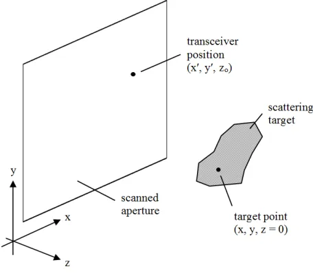
The process of numerically reconstructing a two-dimensional hologram is relatively straightforward. Considering the typical measurement configuration shown in Fig. 1, a transceiver is scanned over the two-dimensional aperture, illuminating the scattering target and measuring the amplitude and phase of the backscattered field [1]. The response measured by the transceiver at z=z0 can be represented by the following two-dimensional Fourier Transform [1]
s(x, y, ω) =
f(x, y, z) exp(−j2kr)dxdy (1)
where each point of the target’s reflectivity functionf(x, y, z) is multiplied by the round trip phase factor and summed at each sample location (x, y, z0), andris given byr=
(x−x)2+ (y−y)2+ (z−z 0)2.
Figure 1. Geometric configuration for holographic imaging system.
In Fig. 1, primed coordinates relate to the aperture plane while unprimed coordinates correspond to the target plane. The phase factor is also a function of wavenumber, denoted as k=ω/c, where ω is the angular frequency and c is the speed of light. The total measured response s(x, y, ω) over the aperture represents a complex hologram record for each frequency ω. The FFT-based reconstruction algorithms for 2-D and 3-D image reconstruction of a target f(x, y) at z0 are given, respectively, by [1]
f(x, y) = FT−2D1[FT2D[s(x, y)] exp{−jKz0}] (2) f(x, y, z) = FT−3D1[FT2D[s(x, y, ω)] exp{−jKz0}] (3)
where FT−3D1 denotes the three-dimensional inverse-FFT operation; FT2D and FT−2D1 indicate the two-dimensional FFT and inverse-FFT operations, respectively; kx,ky, andkz are the planar wavenumbers in thex,y, andzdirections, respectively, which span the range [−2k,+2k]. Also, in Eqs. (2) and (3), we
defineK=
4k2−k2
2.2. Interpolation Schemes
Interpolation is defined as the model-based recovery of continuous data from discrete data within a known range of abscissa values. The main hypotheses related to interpolation are [22]:
(1) The underlying data are continuously defined.
(2) Given data samples, it is possible to compute a data value of the underlying continuous function at any abscissa.
(3) The evaluation of the underlying continuous function at the sampling points yields the same value as the data themselves.
Image interpolation techniques often are required in medical imaging for image generation and processing such as compression or resampling. It transforms a discrete matrix into a continuous image. Subsequent sampling of this intermediate result produces the resampled discrete image [23]. Several interpolating schemes are discussed in detail in [24].
In our analysis, we used the nearest neighbor, linear, and cubic spline interpolation schemes for comparison. Another approach (not tested), namely the cubic convolution interpolation function, is more accurate than the nearest neighbor algorithm or the linear interpolation method. Although not as accurate as a cubic spline approximation, cubic convolution interpolation can be performed much more efficiently [25].
An interpolation scheme is characterized by its kernel function h(x), which represents the convolution operation in the spatial domain [23]. Representative kernel functions used in our work are given by [22, 23]
hNN(x) =
1, 0≤ |x| ≤0.5
0, elsewhere (4)
hLIN(x) =
1− |x|, 0≤ |x| ≤1
0, elsewhere (5)
hCS(x) =
⎧ ⎪ ⎪ ⎪ ⎨ ⎪ ⎪ ⎪ ⎩ 2 3− 1 2|x|
2(2− |x|)
, 0≤ |x|<1 1
6(2− |x|)
3, 1≤ |x| ≤2
0, elsewhere
(6)
for the nearest neighbor (hNN(x)), linear (hLIN(x)), and cubic spline (hCS(x)), respectively.
All interpolation methods smooth the image, and images with sharp-edged details and high local contrast are more affected by interpolation. The nearest neighbor interpolation method, of size 1×1 requiring no mathematical operations, is the fastest technique, but also incurs the largest interpolation error. The linear interpolation method of size 2× 2 requires one addition operation. The cubic spline interpolator is an infinite impulse response (IIR) filter requiring 12 multiplication and 4 addition operations. It produces one of the best results in terms of similarity to the original image. A third-order cubic spline interpolator is usually adequate for most applications [23]. Noise experiments show that the linear interpolation is less sensitive than cubic splines to Gaussian white noise [26]. Its local support and shift-invariant properties offer very attractive computational procedures [27].
2.3. Image Quality Assessment
In order to evaluate the effectiveness of our method, several image quality assessment metrics are used. The first metric used to evaluate reconstructed image quality is mean-squared error (MSE). The MSE is simply the average value of the pixel-to-pixel difference squared, where the image reconstructed fromk out ofN total samples is compared against the ideal reference image reconstructed from allN samples. This relationship is expressed as
MSE = 1
NxNy Nx−1
i=0 Ny−1
j=0
ˆ
Zij −Zij 2
(7)
whereNx is the number of pixels in thex-direction,Ny the number of pixels in they-direction, and ˆZij and Zij are the ideal reference and sparse measured pixel intensities of the (i, j)-th pixel, respectively. One common metric in describing image quality and distortion is peak signal-to-noise ratio (PSNR), which we define in our analysis as
PSNR = 10 log10 ˆ Zmax MSE 2 (8)
where ˆZmax is the maximum possible signal value (for normalized ˆZ, ˆZmax = 1). However, a more appropriate measure of reconstructed image quality is to simply compare the calculated MSE against the MSEmax, which occurs when every pixel from the measured signal is equal to zero (Z = 0). This signal-to-noise ratio (SNR) is calculated as
SNR = 10 log10
MSEmax MSE
(9)
2.4. Resolution Considerations
One of the most important parameters in any imaging application is resolution. For three-dimensional imaging applications, we must consider both the cross-range resolution, as well as the range resolution, the latter also referred to as the down-range resolution.
For the proposed scanned aperture system, the cross-range resolution in the x- and y-directions can be expressed as [21]
δx= λ0R
2Lx (10)
and
δy = λ20LR
y (11)
where λ0 is the wavelength corresponding to the center frequency of the transmitted waveform, R the range to the target, andLx andLy are the sizes of the total scanned aperture in thex- andy-directions, respectively. Note that the cross-range resolution degrades as the range to the target increases and as the aperture size decreases.
The range resolution is solely dependent on the temporal frequency bandwidth of the transmitted waveform and can be expressed as [33]
δz = 2cB (12)
where c is the speed of light, andB is the transmit signal bandwidth. Note that the range resolution degrades as the transmit bandwidth is reduced, and for the limiting case of a monochromatic transmit waveform (B= 0), the range resolution becomes infinite, i.e., targets cannot be resolved in range.
3. SPARSELY SAMPLED RADAR HOLOGRAPHY
Simulated data are produced in MATLAB by importing a binary image and treating every non-zero pixel as an isotropic radiating element. For the scanned aperture in Fig. 1, the total response measured at each detector pixel is simply the summed amplitude and phase from each radiating element of the target model, which is captured by Eq. (1).
3.1. Single-Frequency Image Reconstruction
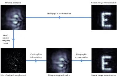
In this section, we discuss the simulation results from sparsely-sampled digital holograms produced by a single frequency. We use the principles discussed in Subsection 2.1 to numerically produce a hologram via computer simulation. The simulated hologram of the letterEof Fig. 2 is 128×128 samples and was generated from a single source frequency of 9.0 GHz. The sampling step sizes in bothx- andy-directions are Δx= Δy= 8.3 mm, resulting in a scanned aperture size of 1.06 m×1.06 m. The target’s simulated distance from the aperture plane was z= 1.5 m. The complex-valued hologram data were then used to
Single frequency holographic reconstruction
Figure 2. Simulated single-frequency hologram, and reconstructed imaged at z = 1.5 m plane using normal image reconstruction.
Holographic reconstruction
Apply random sampling mask
Cubic spline interpolation
Holographic reconstruction
Original hologram Normal image reconstruction
Sparse image reconstruction 10% of original
samples used
Hologram approximation
numerically reconstruct the original target image, which is also shown in Fig. 3. Essentially the same process is used in the X-band holographic radar systems discussed in [18] and [20]. However, as seen in Fig. 3, we have extended our method to include a random sampling process (10% of the data uniformly samples at random) with interpolation prior to reconstruction, significantly reducing the sampling and data acquisition requirements.
The inclusion of the random sampling process can be seen in the simulation experiment of Fig. 3. A single-frequency hologram is produced from a simulated target scene of two humans, one carrying a concealed weapon. Random sampling is performed on the original hologram dataset to produce a subset of data containing only 10% of the original number of samples. After applying a simple cubic spline interpolator to the subsampled dataset, a reconstructed image is produced with a cross-correlation value of ρ= 0.95 against the original reconstructed image.
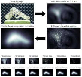
3.2. Wideband Image Reconstruction
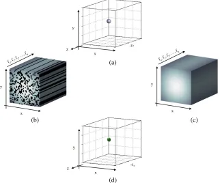
In a real-world holographic imaging system where scan time and data storage requirements are system limitations, our results show that the random sampling paradigm can be very advantageous for X-band applications. Applying these concepts to wideband datasets has been investigated via simulations as well as experiments. Given a distributed, three-dimensional target, wideband holography provides greater depth of field for better imaging resolution [1]. The holographic imaging process is depicted in Fig. 4. A randomly sampled wideband hologram is measured from a simulated target existing within three-dimensional space, as seen in Fig. 4(a). Three-three-dimensional holographic reconstruction is performed only after interpolation to produce a full 3-D datacube of amplitude and phase information for the target in 3-D space [9, 10]. For sparse target scenes, many fewer measurements can be made while still providing enough information for three-dimensional reconstruction, as seen in Fig. 4(d). The amount by which data collection may be reduced depends upon the sparsity of the target to be imaged.
(d) (a)
(b) (c)
4. EXPERIMENTAL RESULTS
4.1. Experimental Setup and Image Reconstruction Results
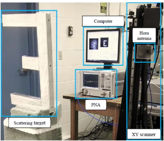
Our experimental setup for holographic measurements primarily consists of a two-dimensional X-Y scanner and network analyzer, as shown in Fig. 5. An Agilent N5225A 50-GHz PNA Network Analyzer was used to collect the data over the scanned aperture, which has a maximum translation length of 90 cm in both x- and y-directions. The network analyzer was used as the transmitter and the receiver. For the data presented in this section, holograms were recorded over the scanned aperture using wideband 2–18 GHz horn antennas whose aperture dimension D was 11.8 cm having an azimuthal beamwidth of approximately 25◦ at the 8-GHz center frequency. The system operated in different modes over frequency ranges of 2–12 GHz, 8.4–11.4 GHz, and 8.4–17 GHz depending on the desired range resolution and sampling step size. The frequency step size used was consistent with a total of 201 frequencies over each band. The sampling interval spacing is dictated by the shortest wavelength used in the step-frequency waveform for a specific application. For example, when operating over the 8.4–11.4 GHz frequency range, we used λ/4 sampling intervals for a step size of 6.6 mm at the highest frequency of 11.4 GHz.
Figure 5. Experimental test setup for holographic imaging system.
4.2. Suppression of Mechanical Vibration Effects
(a)
(b)
Figure 6. (a) Disc shaped median filter of radius 4, and (b) its performance in suppressing high frequency noise caused by scanner vibrations.
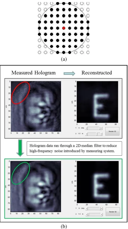
field distribution over the aperture. The median filter was applied prior to sub-sampling, and samples at different percentage values were obtained on this filtered data. Samples were obtained using uniformly sub-sampling at random.
4.3. Single-Frequency Image Reconstruction
The first measurement target was of a letterE measuring 25 cm wide×40 cm tall. The target was built out of wood and wrapped in aluminum foil for enhanced reflectivity. For our system, a raster scan of 16,384 sample points over the entire aperture took approximately 40 minutes. Fig. 7 was produced from a single-frequency slice (11.4 GHz) taken from the wideband data cube. The target object was imaged at a distance of z = 1.5 m from the aperture plane, which measured 128×128 samples across an 84 cm×84 cm scan area.
Figure 7. Comparison of single-frequency holographic reconstruction of letterEfor a normally sampled dataset and a randomly undersampled dataset. The correlation coefficient between the normal and sparse reconstruction images is almost close to unity.
and therefore the difference in the data between the scene containing the target and the background and the scene containing the background alone was due to the target alone. For any practical system, background subtraction is a simple and effective solution at reducing clutter imposed by the stationary measurement environment. Upon applying this reconstruction process to the wideband dataset improved image quality significantly. Image reconstruction with high correlation is achieved with compression ratios even greater than 10 : 1, i.e., using less than 10% of the original number of samples. Larger bandwidths and a greater number of frequencies can provide better range discrimination between target and clutter objects, allowing for better quality reconstruction even in cluttered environments. This is demonstrated in the following section.
4.4. Wideband Image Reconstruction
In order to produce an image of reasonable quality in a cluttered environment, it is necessary not only to meet sampling requirements for spatial resolution in the x-y plane, but is also necessary to have sufficient range resolution in thez-direction. For this reason, wideband imaging is particularly effective in cluttered environments, where discrimination between multiple targets can be accomplished with the proper bandwidth and frequency sampling specifications. In all of the presented results, a basic linear stepped-frequency waveform was used. This waveform was chosen because of its simplicity, low instantaneous bandwidth, and yet high overall bandwidth provided for stretch-processing.
4.4.1. Image Reconstruction of a Simple Target
Preliminary experimentation aimed to demonstrate basic holographic image reconstruction of a metallic object. Measurements were taken in an open indoor environment. For every set of measurement data, background clutter measurement was also recorded to implement background subtraction in order to improve image reconstruction quality as described above.
(b) (a)
(c)
Figure 8. Wideband holographic reconstruction of target E at a distance of 1.5 meters in cluttered environment. (a) Reconstructed image from full dataset. (b) Reconstructed image from only 10% random samples. (c) Progression of reconstructed image quality as number of measurement samples is reduced.
The first target used to demonstrate simple target image reconstruction was constructed in the shape of the capital letter E. This target measured approximately 40 cm×25 cm. The target was imaged over an aperture size of 86.7 cm×86.7 cm with a step-frequency waveform operating over a frequency range from 8.4–11.4 GHz with a bandwidth of 3 GHz. The range to the target was 1.5 m. For this configuration, the cross-range resolutions were computed as 2.62 cm in both the x- and y -directions and the down-range resolution was computed as 5 cm. Results are shown in Fig. 8. Under the environmental conditions for this test setup, 3 GHz of bandwidth was sufficient for imaging of an isolated target. As clutter and other targets of interest are introduced at close proximity, higher signal bandwidth is required in order to prevent spill-over between range bins. Fig. 8 shows the reconstructed image at different values of undersampling, from 91% to 5% of the samples used. Note that the target is well imaged even when using 5% of the samples with a PSNR of 20.33 dB.
Figure 9. Holographic imaging and sparse reconstruction imaging of a prop gun target atz= 0.868 m. The top row shows the image reconstruction process. Note that the gun can be imaged with a PSNR of 32.2 dB even when using 10% of the hologram samples. The middle row shows undersampled holograms at different sampling percentages, and the bottom row shows corresponding image reconstructions.
4.4.2. Image Reconstruction of a Single Concealed Object
Holographic imaging has been used in identifying concealed threat objects. It is pertinent that compressed sensing be applied to the detection process where scanning time may be reduced or 2D antenna arrays may be designed in a simpler and cost-effective manner. In order to demonstrate the benefits of reduced random sampling in this application, threat objects were concealed and imaged at X-band.
Shown in Fig. 10 is an X-band holographic image (8.4–11.4 GHz) of a knife measuring approximately 20 cm in length concealed within a stuffed animal. The down-range resolution was 5 cm. The knife blade is made of stainless steel with a plastic composite handle, and the stuffed animal is made up of polyester with cotton stuffing. Measurements were made with the target at a distance of approximately 64 cm. A scanning aperture of 29.0 cm×39.5 cm yielded a cross range resolution of 3.3 cm and 2.4 cm in the x- and y-directions, respectively. For this particular target setup, it can clearly be seen from the reconstructed images that the concealed threat object can be detected using the holographic imaging technique. Furthermore, a reduction of samples taken of the sparse target scene does not noticeably diminish the recognizability of the concealed weapon in the reconstructed images. A good-quality image is formed even when using 5% of the samples at a PSNR of 20.9 dB.
Figure 10. Holographic imaging and sparse reconstruction at z= 0.636 m of a concealed knife inside a stuffed animal. Sparsely-sampled holograms at different compression ratios and corresponding image reconstructions are shown. The top row shows the stuffed animal, the reconstructed image of the knife using 5% of the samples, and the location of the knife inside the stuffed animal. The middle row shows undersampled holograms at different sampling percentages, and the bottom row shows corresponding image reconstructions.
(b) (a)
(c)
(d)
(e)
(b)
(a) (c)
(d)
(e)
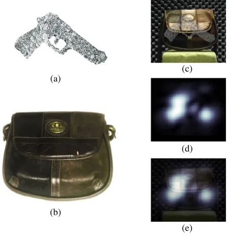
Figure 12. Holographic imaging and reconstruction atz= 0.99 m of prop gun concealed within a soft leather purse. (a) Concealed prop gun. (b) Soft leather purse. (c) Radar view of purse with concealed prop gun. (d) Reconstructed image showing concealed prop gun, and (e) Detected prop gun relative to its location of concealment.
even at a reduced sampling capacity.
In Fig. 12, the prop gun was concealed with a soft leather purse and the bandwidth was extended to 9 GHz (8.4–17.4 GHz) in order to improve the image resolution. The range resolution in this case was 1.67 cm owing to the higher bandwidth. The target was placed at a range of 99 cm. In this case, the cross range resolutions were 1.8 cm and 2.3 cm in thex- andy-directions, respectively. The higher center frequency resulted in a sharpening of the cross range resolutions. It can be seen that the reconstructed holographic image using 5% of the samples from the inside of the second purse reveals a much stronger resemblance of a possible threat object compared to the pervious case. The full outline of the target is visible without gaps.
In order to demonstrate that this imaging technique may be used on a variety of common objects, detection was also tested on a hollow-body acoustic guitar containing a concealed threat object. Fig. 13 shows the uncompressed reconstructed image of the prop gun placed inside of the hollow-body acoustic guitar within the body part, which was located at a range of 52.8 cm. In order to maintain good image resolution, the transmit signal used was a linear stepped-frequency waveform between 2.0–12.0 GHz, yielding a range resolution of 1.5 cm. The high frequencies were able to easily penetrate the hollow wooden guitar. The scan aperture dimensions measured 87.5 cm×55 cm with a measurement step size of 6.25 mm in bothx andy directions. The cross range resolutions in this case were 1.3 cm and 2.06 cm in the x- and y-directions, respectively. In addition to the prop gun, we note that the metallic guitar strings are also imaged well. The brightness of the guitar strings suggests that detection may be difficult if the object is placed beneath the strings. Results from sparse sampling and interpolation of the 3D hologram dataset are also presented in Fig. 14, showing that even for a complex target scene, our sparse sampling reconstruction technique provides excellent image quality for threat object recognition and detection. The PSNR when using 5% of the samples is 20.7 dB.
4.4.3. Image Reconstruction of Multiple Concealed Objects
(b) (a)
(c)
Figure 13. Holographic imaging and reconstruction at z = 0.528 m of prop gun concealed within an acoustic guitar. (a) Acoustic guitar with concealed prop gun within its body, (b) hologram record at 12 GHz, and (c) Reconstructed image showing location of concealed object.
resolution to discriminate between multiple target locations within a 3D volume. This section describes our results on the use of sparse sampling for detection and recognition og multiple concealed objects.
The first case that is considered is a multiple-target setup where a concealed weapon is located inside of a stuffed animal. A leather handbag containing a book and a set of keys is collocated in the z-dimension so as to place both targets within the same range-bin slice. The setup and holographic imaging results can be seen in Fig. 15. The target scene was measured at frequencies 14–17 GHz across an aperture at z = 0 cm with scanned area dimensions of 84.7 cm × 42.4 cm. The range to the target was 68.4 cm. The cross-range resolutions in the x- andy-directions were 0.775 cm and 1.55 cm, respectively, and the down-range resolution was 5 cm. Although invisible to the naked eye, holographic image reconstruction clearly reveals a concealed weapon hidden inside the stuffed animal. Since the reflectivity of the book and keys was much lower than that of the knife, it is difficult to make these shapes out. Also, the purse made of thick leather reduces the amount of transmitted/reflected signal and distorts the image reconstruction due to diffuse scattering. The higher frequency waveform was used to improve spatial resolution, however, penetration was likely reduced, making it difficult to image items inside the purse. However, the threat target is clearly recognized.
The second experiment in this section probes a purse with concealed items inside, including a thick textbook and the prop gun. The size of the measurement aperture in this case was 40 cm×35 cm. This dataset was collected at 401 discrete frequencies between 8.4–17.4 GHz for higher range resolution in order to make it possible to discriminate the gun from the book at different ranges. The thickness of the prop gun measured only to approximately 2 cm, so a range resolution δz of 1.67 cm ensures that the range of the gun does not fall into the same range slice as the book. The images shown in Fig. 16 include the contents to be imaged, the hologram recording, and the reconstructed image produced at a distance of z= 42 cm. Since the wavelength at the center frequency 12.9 GHz is 2.3 cm, the cross-range spatial resolution of the reconstructed image is 1.22 cm and 1.4 cm in the x- and y-directions, making it possible to resolve finer details about the object, such as the trigger cutout.
(a) (b) (c)
Figure 14. Image reconstruction of hollow-body acoustic guitar with concealed weapon at various compression ratios. (a) Undersampled holograms at different percentages of random sampling. (b) Corresponding interpolated holograms, and (c) Corresponding reconstructed images.
(a) (b)
(c)
(d)
(f) (e)
Figure 15. Holographic imaging and reconstruction at z = 0.678 m of prop gun concealed within a stuffed animal which is placed next to a leather handbag containing a book and set of keys. (a) Handbag and objects concealed. (b) Stuffed animal and prop gun concealed within, and (c) Measurement scenario. (d) Radar view of stuffed animal and handbag. (e) Reconstructed image showing detected concealed prop gun, and (f) Detected prop gun relative to its location of concealment.
(c)
(a)
(b)
(e) (d)
(b)
(a)
(d) (c)
Figure 17. Holographic imaging and reconstruction of prop gun at z = 0.99 m and a sweatshirt concealed within a backpack. (a) Backpack and objects concealed. (b) Radar view of backpack with objects placed within. (c) Reconstructed image showing detected concealed knife, and (d) Detected knife relative to its location of concealment.
total ofN = 2,387,880 samples for the complete dataset. At a constant sampling interval ofλ/4, this is the amount of data that would typically be expected to produce an image of such a target scene given the waveform parameters. However, it is demonstrated in an empirical sense by the images reconstructed at different compression ratios. The cross-range resolutions were 2.41 cm and 1.64 cm in the x- and y-directions, respectively, while the down-range resolution was 5 cm. We see that even when using 5% of the samples, the presence of the concealed knife is still extracted in the image. This effectively allows for higher resolution images without requiring an extensive amount of data to be collected.
4.4.4. 3-D Image Reconstruction of Multiple Concealed Objects
Experiments were conducted in order to demonstrate that concealed targets located at different ranges can be resolved and identified. A cardboard box filled with paper measuring 20 cm wide ×30 cm long ×25 cm high was used to conceal metallic objects placed in different locations in space. Targets used include a steel wrench, measuring approximately 25 cm long, a pocket knife measuring approximately 15 cm long, and the prop gun measuring approximately 20 cm long.
The wrench and prop gun were spaced approximately 18 cm apart in the z-direction at opposite sides of the box. As shown in Fig. 18, these objects were spaced 15 cm apart from one another in the cross-range direction to avoid shadowing. A stepped-frequency waveform between 2–12 GHz was used to achieve a down-range resolution of 1.5 cm, more than adequate to separate the range-separated targets. An aperture size of 40 cm×35 cm was used. At a range of 36.4 cm where the wrench was located, the cross-range resolutions were 1.4 cm and 1.6 cm in the x- and y-directions, respectively. At a range of 54 cm where the prop gun was located, the cross-range resolutions were 2.0 cm and 2.3 cm in thex- and y-directions, respectively. Sparse holographic image reconstruction of targets in 3D space using 5% of the samples also shown in Fig. 19 demonstrates that high resolution images may be obtained with many fewer samples.
Figure 19 shows sparse holographic image reconstruction of the wrench and the prop gun inside the cardboard box 1 for different compression ratios. We note that even at 5% compression ratio, we are able to achieve a PSNR of great than 23 dB.
(c)
(a) (b)
(d) (e)
Figure 18. Holographic reconstruction of concealed objects within cardboard box 1 showing image of wrench and prop gun reconstructed. (a) Top view of open box showing location of concealed prop gun and wrench. (b) Top view of box prior to closing lid. (c) Position of concealed objects. (d) Reconstructed image of wrench at z= 0.364 m, and (e) Reconstructed image of prop gun at z= 0.540 m.
(c) (a)
(b)
(f) (d)
(e)
Figure 20. Holographic reconstruction of concealed objects within cardboard box 2 showing image of wrench reconstructed at z = 0.375 m, image of knife reconstructed at z = 0.493 m, and image of prop gun reconstructed at z = 0.623 m. (a) Top view of open box showing location of concealed objects. (b) Top view of box prior to closing lid. (c) Position of concealed objects. (d) Reconstructed image of wrench at z = 0.375 m. (e) Reconstructed image of knife at z = 0.493 m, and (f) reconstructed image of prop gun at z= 0.623 m.
equipment, high waveform frequencies may provide better target imaging resolution at the cost of smaller sampling step sizes. An aperture size of 40 cm×35 cm was used. At a range of 37.5 cm where the wrench was located, the cross-range resolutions were 1.4 cm and 1.6 cm in the x- and y-directions. At a range of 49.3 cm where the knife was located, the cross-range resolutions were 1.9 cm and 2.1 cm in the x- and y-directions. At a range of 62.3 cm where the prop gun was located, the cross-range resolutions were 2.4 cm and 2.7 cm in thex- andy-directions. Sparse holographic image reconstruction of targets in 3D space when using 5% of the samples shown in Fig. 20 demonstrates that high resolution images may be obtained with many fewer samples.
4.5. Noise Considerations
microwave imaging system. The Agilent N5225A 50 GHz PNA Network Analyzer used has a noise floor of −117 dBm at 10 Hz IF bandwidth. For our near-field imaging system operating at 0 dBm transmit power, this level of noise is essentially negligible.
In a sparse holographic imaging system, missing pixel information prevents the use of common spatial filtering techniques. However, the step at which pixel values are determined via interpolation effectively serves as a lowpass filter process. In order to evaluate the effects of noise induced on sparse measurement data prior to reconstruction, three sets of data were evaluated. Fig. 21 shows reconstructed images of the prop gun with various noise levels added prior to reconstruction. The corresponding plot of the SNR at different compression ratios is shown in Fig. 22. For each dataset, SNR was measured at
(a)
(c)
Figure 21. Reconstructed images of prop gun with various noise levels added prior to sparse reconstruction pertaining to (a) Fig. 9, (b) Fig. 13, and (c) Fig. 18.
different compression ratios for various levels of noise added to the hologram (40 dB, 30 dB, and 20 dB noise floor). When a large amount of data pixels were collected, the SNR was affected at the same scale as the amount of noise introduced. As the hologram samples became sparser, the noise had less influence on the overall SNR of the reconstructed image. In one respect, the sparser the dataset, the less influence the additive noise has on the reconstructed image. Values of missing pixels are estimated via interpolation of a cubic spline function between existing data and are therefore not subjected to high frequency noise.
4.6. Interpolation Considerations
In contrast to the common alternative methods for sparsity-based signal estimation (such as total variation and 1-norm minimization), our processing scheme is much faster. Although the full dataset would not need to be collected in practice, quantitative evaluation of the effectiveness of this modified reconstruction process requires a reference signal (image) to provide a baseline for comparative quality metrics. In our evaluation, we compared sum of absolute differences (SAD, also known as the1-norm), mean-squared error (MSE, also known as the 2-norm), and SNR versus compression ratio for three different interpolation schemes: linear, cubic spline, and nearest neighbor. Compression ratio is simply the inverse of the number of samples used in the undersampled subset.
Figure 23 shows an example of our results pertaining to the case considered in Fig. 10. A comparison of reconstruction using different interpolation methods applied prior to reconstruction is shown. Also shown are the three metrics considered, namely, PSNR,1-norm, and2-norm versus compression ratio. The performance of each interpolation scheme was considered for each of the 14 experimental datasets and was averaged over the 14 datasets to produce the plots seen in Fig. 24. From these results, we conclude that the cubic spline interpolation scheme is most effective in sparse holographic image reconstruction. However, depending on the sparsity of the target scene, satisfactory image reconstruction quality may vary with compression ratio. With this in mind, a system may be designed using the sparse holographic reconstruction technique to meet desired image resolution and noise floor specifications while benefiting from the drastic reduction in sampling requirements.
(b)
Figure 23. (a) Comparison of interpolation methods applied prior to reconstruction for case shown in Fig. 10. (b) PSNR,1-norm, and 2-norm versus compression ratio.
5. CONCLUSIONS
Wideband holographic imaging is an effective means for gathering information from three-dimensional target scenes. Through simulation and experimentation, we have verified that for low-frequency hologram records, simple interpolation of sparsely-sampled target scenes provides a quick and reliable approach to reconstruct sparse datasets for accurate image reconstruction.
For scanning radar applications, data collection time can be drastically reduced through application of sparse sampling. This reduced scan time will typically benefit a real-time system by allowing improvements in processing and decision-making algorithms. Furthermore, the reduction of required data storage as earned value may afford better design specifications in other aspects of a holographic measurement system. Sparse holographic reconstruction may also provide advantages when considering the design of a two-dimensional antenna array. Although the actual benefits accruing in computational costs, both processing and storage, will depend upon the user’s processing platform, it is obvious that a considerable advantage will be gained by collecting and processing a subset of the data.
By reducing the number of detector elements, a direct decrease in material cost is achieved, as well as a reduction in complexity for the transmission line network and supporting elements. This study has considered the significance of interpolation techniques applied to digital holography with low spatial frequency prior to image reconstruction. Results have demonstrated that this is highly effective when imaging target scenes can be represented in some sparse domain. Future work includes theoretical analysis of reconstruction performance under different clutter scenarios, noise levels, and target complexity, and a comparison with traditional compressive imaging approaches. Future system development may consider different transceiver antennas, signal bandwidths, as well as possible fusion of sparse sampling, interpolation, and1-norm minimization techniques for holographic processing and image reconstruction.
ACKNOWLEDGMENT
This work was partially supported by US Air Force Office of Scientific Research Grant number FA9550-12-1-0164. We appreciate helpful suggestions from Mahesh Shastry of Oregon Health and Science University (OHSU).
REFERENCES
1. Sheen, D. M., D. L. McMakin, and T. E. Hall, “Three-dimensional millimeter-wave imaging for concealed weapon detection,” IEEE Trans. Microwave Theory Tech., Vol. 49, No. 9, 1581–1592, Sep. 2001.
2. Goodman, J. W., Introduction to Fourier Optics, McGraw-Hill, New York, NY, 1968.
3. Brady, D. J., K. Choi, D. L. Marks, R. Horisaki, and S. Lim, “Compressive holography,” Opt. Express, Vol. 17, No. 15, 13040–13049, Jul. 20, 2009.
4. Cand`es, E. and J. Romberg, “Sparsity and incoherence in compressive sampling,” Inverse Prob., Vol. 23, No. 3, 969–985, Jun. 2007.
5. Rivenson, Y. and A. Stern, “Compressive sensing techniques in holography,” in Proc. 10th Euro-Am. Workshop Inf. Opt. (WIO), Benic`assim, Spain, Jun. 2011, doi: 10.1109/WIO.2011.5981451. 6. Hald, J., “Wideband acoustical holography,” Proc. 43rd Int. Congress Noise Control Eng., 44–56,
Melbourne, Australia, Nov. 2014.
7. Qiao, L., Y. Wang, Z. Shen, Z. Zhao, and Z. Chen, “Compressive sensing for direct millimeter-wave holographic imaging,” Appl. Opt., Vol. 54, No. 11, 3280–3289, Apr. 10, 2015.
8. Cull, C. F., D. A. Wikner, J. N. Mait, M. Mattheiss, and D. J. Brady, “Millimeter-wave compressive holography,” Appl. Opt., Vol. 49, No. 19, E67–E82, Jul. 1, 2010.
10. Demirci, S., H. Cetinkaya, E. Yigit, C. Ozdemir, and A. Vertiy, “A study on millimeter-wave imaging of concealed objects: application using back-projection algorithm,” Progress In Electromagnetics Research, Vol. 128, 457–477, 2012.
11. Harmer, S. W., N. J. Bowring, N. D. Rezgui, and D. Andrews, “A comparison of ultra wide band conventional and direct detection radar for concealed human carried explosives detection,”Progress In Electromagnetics Research Letters, Vol. 39, 37–47, 2013.
12. Yurduseven, O., “Indirect microwave holographic imaging of concealed ordnance for airport security imaging systems,”Progress In Electromagnetics Research, Vol. 146, 7–13, 2014.
13. Wilson, S. A. and R. M. Narayanan, “Compressive wideband microwave radar holography,”Proc. SPIE Conf. Radar Sensor Technol. XVIII, Baltimore, MD, May 2014, 907707-1–907707-8.
14. Wilson, S. A., R. M. Narayanan, and M. Rangaswamy, “Wideband imaging of concealed objects using compressive radar holography,” Proc. IEEE Int. Radar Conf., 925–930, Arlington, VA, May 2015.
15. Gabor, D., “A new microscopic principle,”Nat., Vol. 161, No. 4098, 777–778, May 15, 1948. 16. Soumekh, M., “Bistatic synthetic aperture radar inversion with application in dynamic object
imaging,”IEEE Trans. Signal Process., Vol. 39, No. 9, 2044–2055, Sep. 1991.
17. Ida, Y., K. Hayashi, and K. Ami, “The effect of reference’s phase on radio-frequency holographic imaging,”IEEE Trans. Antennas Propag., Vol. 30, No. 6, 1216–1221, Nov. 1982.
18. Ivashov, S., V. Razevig, A. Sheyko, I. Vasilyev, A. Zhuravlev, and T. Bechtel, “Holographic subsurface radar technique and its applications,” Proc. 12th Int. Conf. Ground Penetrating Radar, 1–11, Birmingham, UK, Jun. 2008.
19. Collins, H. D., D. M. Sheen, T. E. Hall, and R. P. Gribble, “UWB radar holography applied to RCS signature reduction of military vehicles,”Rev. Prog. Quant. Nondestr. Eval., Vol. 16, 703–707, 1997.
20. Zhuravlev, A., S. Ivashov, V. Razevig, I. Vasiliev, and T. Bechtel, “Shallow depth subsurface imaging with microwave holography,”Proc. SPIE Conf. Detect. Sens. Mines, Explos. Objects, and Obscured Targets XIX, 90720X-1–90720X-9, Baltimore, MD, May 2014.
21. Hunt, J., J. Gollub, T. Driscoll, G. Lipworth, A. Mrozack, M. S. Reynolds, D. J. Brady, and D. R. Smith, “Metamaterial microwave holographic imaging system,”J. Opt. Soc. Am. A, Vol. 31, No. 10, 2109–2119, Oct. 2014.
22. Th´evenaz, P., T. Blu, and M. Unser, “Image interpolation and resampling,” Handbook of Medical Image Processing and Analysis, 2nd Edition, 465–493, edited by I.N. Bankman, Academic Press, Burlington, MA, 2009.
23. Lehmann, T. M., C. Gonner, and K. Spitzer, “Survey: interpolation methods in medical image processing,” IEEE Trans. Med. Imaging, Vol. 18, No. 11, 1049–1075, Nov. 1999.
24. Th´evenaz, P., T. Blu, and M. Unser, “Interpolation revisited,”IEEE Trans. Med. Imaging, Vol. 19, No. 7, 739–758, Jul. 2000.
25. Keys, R., “Cubic convolution interpolation for digital image processing,” IEEE Trans. Acoust. Speech Signal Process., Vol. 29, No. 6, 1153–1160, Dec. 1981.
26. Herman, G. T., S. W. Rowland, and M.-M. Yau, “A comparative study of the use of linear and modified cubic spline interpolation for image reconstruction,” IEEE Trans. Nucl. Sci., Vol. 26, No. 2, 2879–2984, Apr. 1979.
27. Hou, H. S. and H. Andrews, “Cubic splines for image interpolation and digital filtering,” IEEE Trans. Acoust. Speech Signal Process., Vol. 26, No. 6, 508–517, Dec. 1978.
28. Parker, J. A., R. V. Kenyon, and D. E. Troxel, “Comparison of interpolating methods for image resampling,” IEEE Trans. Med. Imaging, Vol. 2, No. 1, 31–39, Mar. 1983.
29. Donoho, D. L. and J. Tanner, “Precise undersampling theorems,” Proc. IEEE, Vol. 98, No. 6, 913–924, Jun. 2010.
31. Cand`es, E. J. and M. B. Wakin, “An introduction to compressive sampling,”IEEE Signal Process. Mag., Vol. 25, No. 2, 21–30, Mar. 2008.
32. Rivenson, Y. and A. Stern, “Compressive holography,” Optical Compressive Imaging, edited by A. Stern, 155–176, CRC Press, Boca Raton, FL, 2017.
33. Keep, D. N., “Frequency-modulation radar for use in the mercantile marine,” Proc. IEE — Part B: Radio Electron. Eng., Vol. 103, No. 10, 519–523, Jul. 1956.
34. J¨ahne, B., Digital Image Processing: Concepts, Algorithms, and Scientific Applications, 3rd Edition, Springer-Verlag, London, UK, 2002.
35. Du, K., H. Han, and G. Wang, “A new algorithm for removing compression artifacts of wavelet-based image,”Proc. 2011 IEEE Int. Conf. Comput. Sci. Autom. Eng. (CSAE), 336–340, Shanghai, China, Jun. 2011.
36. Akey, M. L. and O. R. Mitchell, “Detection and sub-pixel location of objects in digitized aerial imagery,” Proc. 7th Int. Conf. Pattern Recognit., 411–414, Montr´eal, Canada, Jul.–Aug. 1984. 37. Daniels, D. J., D. J. Gunton, and H. F. Scott, “Introduction to subsurface radar,” IEE Proc. Part
F: Radar Signal Process., Vol. 135, No. 4, 278–320, Aug. 1988.