Precision physics with QCD

Precision physics with QCD

Antonio Pich1,a

1_{Departament de Física Teòrica, IFIC, Universitat de València – CSIC} Edifici d’Instituts de Paterna, Apt. Correus 22085, E-46071, València, Spain

Abstract.The four-loop determination of the strong coupling from fully inclusive ob-servables is reviewed. Special attention is given to the low-energy measurement ex-tracted from the hadronicτdecay width. A recent exhaustive analysis of the ALEPH data, exploring several complementary methodologies with very different sensitivities to inverse power corrections and duality violations, confirms the strong suppression of non-perturbative contributions toRτ. It gives the valueαs(m2τ)=0.328±0.013, which implies

αs(MZ2) = 0.1197±0.0015. The excellent agreement with the direct measurement at

theZpeak,αs(M2Z)=0.1196±0.0030, provides a beautiful test of asymptotic freedom.

Together with the most recent lattice average from FLAG and the NNLO determinations frome+e−

, PDFs and collider data quoted by the PDG, these two inclusive determinations imply a world average valueαs(M2Z)=0.1180±0.0010.

1 Introduction

All strong interaction phenomena should be described in terms of the strong couplingαs, the single free parameter of Quantum Chromodynamics (QCD). The overwhelming consistency of the many de-terminations ofαs, performed in different processes and at different mass scales provides a beautiful verification of QCD. A good understanding of the uncertainties associated with the different measure-ments is needed in order to appreciate the significance of this test, which must be then restricted to observables where perturbative techniques are reliable and enough terms in the perturbative expan-sion are available. The PDG [1] requires a NNLO (or higher) theoretical accuracy. In addition, small non-perturbative corrections are always present, specially at low energies, and one should also worry about the expected asymptotic behaviour of the perturbative series.

The most reliable determinations ofαshave been compiled in Refs. [2–6]. I will focus the discus-sion on the very precise inclusive observablesRZandRτ, which are already known to four loops,i.e., to N3LO, and will update the PDG information with the most recent developments, not yet included in the official averages.

2 Running coupling and effective QCD theories

The QCD coupling obeys the renormalization group equation

µdαs(µ2)

dµ = αs(µ

2_)β(α

s), β(αs) =

X

n=1

βnans, as = αs

π . (1)

1 5 10 50 100 0.1 0.2 0.3 0.4 0.5

E ₍GeV₎

αs

(

E

2 )

1 5 10 50 100

0.1 0.2 0.3 0.4 0.5

E ₍GeV₎

αs

(

E

2 )

2.30 2.35 2.40 2.45 2.50

0.260 0.265 0.270 0.275 0.280 0.285 0.290

αs(m2τ) = 0.328±0.013

N4LO N3LO N2LO NLO LO

A. Pich Precision Physics with QCD 1

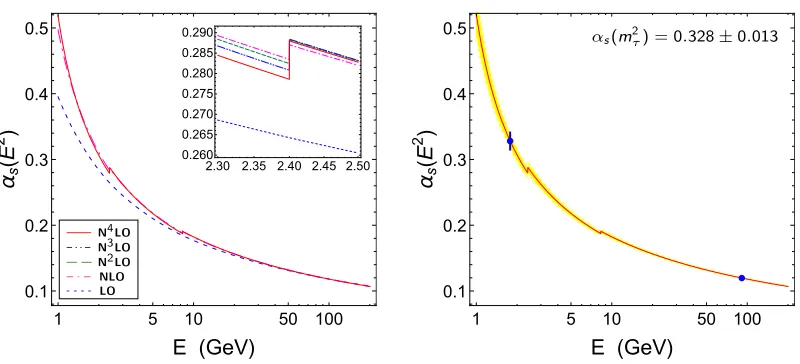
Figure 1. Scale dependence ofαs at different perturbative orders (left). The right plot compares the 5-loop

evolution ofαs(m2τ), determined from hadronicτdecays, with the measurement ofαs(M2Z) fromΓZ.

The fifth-order coefficient of theβfunction has been recently computed in Ref. [7] (see also Ref. [8]), which provides a quite precise perturbative control of the scale dependence ofαs. In the MS scheme (β1andβ2are scheme independent), the known coefficients are [7, 9, 10]:

β1 = 1 3nf−

11

2 , β2 = −

51 4 +

19

12nf, β3 = 1 64

"

−2857+5033 9 nf −

325 27 n 2 f # ,

β4 = −1

128 "

149753

6 +3564ζ3−

1078361 162 +

6508 27 ζ3

! nf+

50065 162 +

6472 81 ζ3

!

n2_f+1093 729 n

3 f

#

,

β5 = − 1

512 (

8157455

16 +

621885 2 ζ3−

88209

2 ζ4−288090ζ5

+nf

"

−336460813

1944 −

4811164 81 ζ3+

33935 6 ζ4+

1358995 27 ζ5

#

+n2_f "

25960913 1944 +

698531 81 ζ3−

10526 9 ζ4−

381760 81 ζ5

#

+n3_f "

−630559

5832 − 48722

243 ζ3+ 1618

27 ζ4+ 460

9 ζ5 #

+n4_f " 1205 2916− 152 81 ζ3 # ) . (2)

The very modest growth ofβnwith the perturbative order gives rise to a surprisingly smooth power expansion. Fornf =5, for instance,β(αs)=β1as

1+1.26as+1.47a2s+9.83a3s+7.88a4s

.

The scale dependence ofαsover a wide range of energies, at different levels of approximation, is shown in figure 1. The 5-loop precision in theβfunction implies a resummation of N4_{LO logarithmic}

The small discontinuities in the plotted curves reflect the crossing of the charm and bottom thresh-olds where one needs to properly match the different QCDnf effective theories. Since theβncoeffi

-cients are functions ofnf, the strong coupling depends on the considered number of “active” quark flavours. When a quark is heavy enough to decouple, it is convenient to remove it from the La-grangian and work with an effective QCD theory which has one quark less and a different value ofαs. The matching conditions relating the effective QCD theories withnf andnf−1 flavours are known to four loops [11, 12].

3 Inclusive observables

Inclusive observables, such asσ(e+e− _{→ hadrons) at high-enough energies, Γ(Z → hadrons) or}

Γ(W → hadrons), can be accurately predicted with perturbative methods. Since the final hadrons are produced through the vector V_{i j}µ=ψ¯jγµψi and axial-vector Aµ_{i j} =ψ¯jγµγ5ψi colour-singlet quark currents (i,j=u,d,s. . .), the QCD dynamics is governed by the two-point correlation functions

Πµν_{i j,J}(q) ≡ i Z

d4x eiqxh0|T(J_{i j}µ(x)Jν_{i j}(0)†)|0i = −gµνq2+qµqνΠ(0_{i j,}+_J1)(q2)+gµνq2Π(0)_{i j,J}(q2), (3)

whereJ = V,A and the superscript L = 0,1 denotes the angular momentum in the hadronic rest frame. The correlatorsΠ(_{i j}L_,)_J(q2_{) are analytic functions ofq}2_{, in the complexq}2_{plane, except along the}

(physical) positive real axis where their imaginary parts have discontinuities which correspond to the measurable hadronic spectral distributions with the given quantum numbers.

For massless quarks,sΠ(0)_{i j,J}(s)=constant (there is a non-perturbative Goldstone-pole contribution

toΠ(0)_{i j,A} ats= 0, which cancels inΠ(0_{i j,}+_A1)). Wheni , j, the two quark currents must necessarily be

connected through a quark loop (non-singlet topology), which gives identical contributions to the vec-tor and axial massless correlavec-tors:Π(s)≡Π(0_i +1)

,j,V(s)= Π (0+1)

i,j,A(s). They are conveniently parametrized through the Euclidean Adler function (Q2_=−q2_andN

C=3 is the number of quark colours)

D(Q2) ≡ −Q2 d dQ2Π(Q

2_{) =} NC 12π2

      

1+X n=1

Kn

αs(Q2) π

!n      

, (4)

which is known toO(α4

s) [13–15]:

K1 = 1, K2 = 1.98571−0.115295nf, K3 = 18.2427−4.21585nf +0.0862069n2f,

K4 = 135.792−34.4402nf +1.87525n2f −0.0100928n 3

f. (5)

There are additional singlet contributions to the neutral-current correlators (i= j), with each current coupling to a different quark loop. Since gluons haveJPC ₌₁−−_{and colour, these topologies start to}

contribute atO(α3

s) andO(α2s), respectively, for the vector and axial-vector currents:

∆S

DV(Q2) = NC 12π2

X

n=3

dnV

αs(Q2) π

!n

, ∆S

DA(Q2) = NC 12π2

X

n=2

dAn

αs(Q2) π

!n

. (6)

The vector-current coefficients aredV

3 =−0.41318 andd V

The ratio of the electromagnetice+e−→hadrons ande+e−→µ+µ−cross sections is given by

Re+e−(s) ≡

σ(e+e−_→hadrons)

σ(e+e−_→µ+µ−₎ = 12π

         X f

Q2_f ImΠ(s)+         X f Qf         2

Im∆SΠV(s)

         = X f Q2_f NC

      

1+X n≥1

Fn αs(s)

π

!n       + O       

m2q

s , Λ4 s2      

. (7)

The sum over quark electric charges of different signs strongly suppresses the singlet contribution, which has been included as a small correction to the coefficientsFn≥3. Fornf =5 flavours, one gets F1 =1,F2=1.4092,F3=−12.805 andF4=−80.434 [16].

The perturbative series in Eq. (7) is actually an expansion in powers ofαs(µ2) with coefficients containing a polynomial dependence on log (s/µ2_{). These logarithms are resummed into the running}

coupling by takingµ2 _{=s. Although the physical ratioR}

e+e−(s) is independent of the renormalization

scaleµ, the truncated series contains a residual µ-dependence ofO(αN+1

s ), where N = 4 is the last included term, which must be taken into account in the theoretical uncertainty. Since non-perturbative corrections are suppressed byΛ4_/s2 _{(the gauge-invariant operators contributing to the current}

corre-lators have dimensions D ≥ 4), at high energies one can perform a N3LO determination ofαs(s). Unfortunately, the experimental uncertainties are large.

3.2 Γ(Z →hadrons)

The electroweak neutral currentJµ_Z=P

f(vfVµ_{f f}+afAµ_{f f}) contains vector and axial-vector components, weighted with the correspondingZ couplings. The singlet axial contributions of the two members of a weak isospin doublet cancel each other for equal quark masses becauseaf =2If; however, the large value of the top mass generates very important singlet axial corrections which start atO(α2_s). The ratio of the hadronic and electronic widths of theZboson involves the QCD series (mb=0,mt,0)

RZ ≡ Γ

(Z→hadrons)

Γ(Z →e+e−₎ = R

EW Z NC

      

1+X n=1

˜ Fn      

αs(M2Z) π       n       , (8)

with ˜F1=1, ˜F2=0.76264, ˜F3 =−15.490 and ˜F4=−68.241 [16]. Taking properly into account the

electroweak corrections and QCD contributions suppressed by powers ofm2_b/M2_Z [17, 18], the ratio RZis included in the global fit to electroweak precision data. This results in a quite accurate value of αs(M2_Z) [19]:

α(nf=5)

s (MZ2) ≡ αs(M2Z) = 0.1196±0.0030. (9)

This determination assumes the validity of the electroweak Standard Model.

4 Hadronic decay width of the

τ

lepton

Figure 2.Spectral functions for theV,AandV+Achannels, determined from ALEPHτdata [26].

QCD correlation function of two left-handed charged currents receives only non-singlet contributions. Restricting the analysis to the dominant Cabibbo-allowed decay width,

Rτ,V+A ≡

Γ[τ−_→ν

τ+hadrons (S =0)] Γ[τ−_→ν_τe−ν_¯

e]

(10)

= 12π|Vud|2SEW

Z m2 τ

0

ds m2

τ

1− s

m2

τ !2

1+2 s m2

τ !

ImΠ(0_ud+_,V1)_+A(s)−2 s m2

τ

ImΠ(0)_ud,V+A(s)

,

whereSEW = 1.0201±0.0003 incorporates the electroweak radiative corrections [23–25]. The

measured invariant-mass distribution of the final hadrons determines the spectral functionsρJ(s) ≡ 1

πImΠ

(0+1)

ud,J (s), shown in figure 2 (the only relevant contribution to thesImΠ 0

ud,V+A(s) term is theπ

−

final state ats=m2

π).

Using the analyticity properties of theΠ(_{i j}L_,)_J(s) correlators, the experimental spectral distribution can be related with theoretical QCD predictions through moments of the type [22, 27]

Aω_J(s0) ≡

Z s0

sth ds

s0

ω(s) ImΠ(0₊1) ud,J (s) =

i 2

I

|s|=s0 ds

s0

ω(s)Π(0_ud+_,J1)(s), (11)

wheresthis the hadronic mass-squared threshold,ω(s) is any weight function analytic in|s| ≤s0, and

the complex integral in the right-hand side (rhs) runs counter-clockwise around the circle|s|=s0. For

large-enough values ofs0, the operator product expansion (OPE)

Π(0+1) ud,J(s)

OPE ₌ X

D 1 (−s)D/2

X

dimO₌D

CD,J(−s, µ)hO(µ)i ≡

X

D O_D,J

(−s)D/2, (12)

can be used to predict the rhs integral as an expansion in inverse powers ofs0(theD=0 term contains

the perturbative contribution), while the lhs is directly determined by the experimental data.

The ratio Rτ,V+A in Eq. (10) corresponds to the particular weight ω(x) = (1− x2)(1 +2x) = 1−3x2_+2x3_{, withx≡s/s}

0ands0=m2τ. Thus, owing to Cauchy’s theorem, the contour integral is only sensitive to OPE corrections withD=6 and 8, which are strongly suppressed by the corresponding powers of theτmass (there is in addition a further suppression of theD=6 term because the vector and axial-vector contributions have opposite signs, cancelling to a large extent). Moreover,ω(s) contains a double zero ats = s0 which heavily suppresses the contribution to the integral from the

Method αs(m2τ)

CIPT FOPT Average

ALEPH moments 0.339₋+0_0..019₀₁₇ 0.319+₋₀0_..017₀₁₅ 0.329+₋0₀._.020₀₁₈

Modified ALEPH moments 0.338+0.014

−0.012 0.319+ 0.013

−0.010 0.329+ 0.016

−0.014

A(2,m)moments 0.336₋+0₀._.018₀₁₆ 0.317+₋0₀._.015₀₁₃ 0.326+₋0₀._.018₀₁₆

s0dependence 0.335±0.014 0.323±0.012 0.329±0.013

Borel transform 0.328₋+0_0..014₀₁₃ 0.318+₋₀0_..015₀₁₂ 0.323+₋0₀._.015₀₁₃

The availability of good experimental data makes possible to determine the small non-perturbative corrections from the data themselves, using weights with different powers of swhich are sensitive to the corresponding power corrections in the OPE [27]. The dominant uncertainty in theαs(m2τ) determination comes from the perturbative error associated with the unknown higher-order corrections to the Adler series in Eq. (4). For a given value ofαs, the so-called contour-improved perturbation theory (CIPT) [28, 29], which resumms large corrections arising from the long running along the circle s=s0, results in a smaller perturbative contribution than the truncated fixed-order perturbation theory

(FOPT) approximation [22]. Therefore, CIPT leads to a larger fitted value ofαs(m2τ) than FOPT.

4.1 Numerical analysis

A detailed reanalysis of theαs(m2τ) determination fromτdecay has been recently performed [30], in-cluding many consistency checks to assess the potential size of non-perturbative effects. All strategies adopted in previous works have been investigated, studying the stability of the results and trying to un-cover any potential hidden weaknesses, and several complementary approaches have been considered. Once their uncertainties are properly estimated, all adopted methodologies result in very consistent values ofαs(m2τ). Table 1 summarizes the most reliable determinations.

All analyses have been done both in CIPT and FOPT. Within a given approach the perturbative errors have been estimated varying the renormalization scale in the intervalµ2/s0 ∈ [0.5,2], and

taking K5 = 275±400 as an educated guess of the maximal range of variation of the unknown

fifth-order contribution [31]. These two sources of theoretical uncertainty have been combined in quadrature, together with the experimental errors. The different values quoted in the table include, as an additional uncertainty, the variations of the results under various modifications of the fit procedures. The systematic difference between the values obtained with the CIPT and FOPT prescriptions appears clearly manifested in the table. The CIPT and FOPT results have been finally averaged, but adding in quadrature half their difference to the smallest of the CIPT and FOPT errors.

The first determination in table 1 follows the method adopted in the ALEPH analysis of Ref. [26], taking the weightsωkl(x) = (1−x)2+kxl(1+2x) with (k,l) = {(0,0),(1,0),(1,1),(1,2),(1,3)}and s0 =m2τ. With five moments, one can make a global fit ofαs(m2τ), the gluon condensate,O6andO8.

To assess possible errors associated with neglected higher-order condensates, a second fit including

O10has been performed and the variation on the fitted value of the strong coupling has been included

as an additional uncertainty. A quite precise value ofαs(m2τ) is obtained, in good agreement with Ref. [26]. The extracted condensates have large relative errors exhibiting a very little sensitivity to power corrections. This has been further verified, taking away from the weights the factor (1+2x) which eliminates the highest-dimensional condensate contribution to every moment. This gives the

Table 1.Determinations ofα(nf=3)

Figure 3.Dependence ons0of the experimental momentsA(1,0)_{(s0) (left) andA}(2,0)_{(s0) (right), together with their} purely CIPT and FOPT perturbative predictions forα(nf=3)

s (m2τ)=0.329+−00..020018. Data points are shown for theV (red),A(green) and1

2(V+A) (blue) channels. The horizontal (pink) line indicates the free-parton result [30].

fitted values shown in the second line of table 1, which are in perfect agreement with the results of the previous fit (first line) and are even more precise.

The doubly-pinched weightsω(2,m)(x)=(1−x)2Pm

k=0(k+1)x

k_=1−(m+2)xm₊1_+(m+1)xm₊2

are only sensitive toO2(m+2)andO2(m+3). A combined fit of five differentA(2,m)moments (1≤m≤5)

gives the results shown in the third line of table 1. First, a global fit with four free parameters, assumingO₁₂ = O₁₄ = O₁₆ = 0, has been done. To account for these missing power corrections, the fit has been repeated with the inclusion ofO₁₂ and the variation in the fitted value ofαs(m2τ) has been taken as an additional uncertainty. The agreement with the results obtained in the previous fits is excellent. Similar results (not included in the table) are obtained from a global fit to fourA(n,0)

(0≤n≤3) moments based on the n-pinched weightsω(n,0)_(x)=(1−x)n_{which receive corrections} from all condensates withD≤2(n+1), but are protected against duality violations forn,0.

Neglecting all non-perturbative effects, one can determineαs(m2τ) from a single moment. This interesting exercise has been also done in Ref. [30], making 13 separate extractions of the strong coupling with sixA(2,m)_{moments (0≤m≤5), sixA}(1,m)_{moments (0≤m≤5) based on the weights} ω(1,m)_{(x) = 1−x}m+1 _{= (1−x)}Pm

k=0xk which are only sensitive toO2(m+2), and the momentA(0,0)

where OPE corrections are absent but it is very exposed to duality-violation effects. In all cases, the resulting determinations of the strong coupling are in agreement with the values in table 1, reflecting the minor numerical role of the neglected non-perturbative corrections.

Non-perturbative contributions should manifest in a distinctives0dependence. Figure 3 shows as

function ofs0the experimental momentsA(1,0)(s0) andA(2,0)(s0), in theV,Aand 1₂(V+A) channels,

together with their predicted values withα(nf=3)

s (m2τ) = 0.329−+00..020018, neglecting all non-perturbative

contributions. A(1,0)_(s

0), which can only get corrections fromO4, exhibits a surprisingly good

agree-ment with its pure perturbative prediction. In spite of being only protected by a single pinch factor, the data points aboves0 ∼2 GeV2closely follow the central values predicted by CIPT. In that energy

range non-perturbative contributions appear to be too small to become numerically visible within the much larger perturbative uncertainties covering the shades areas of the figure. The splitting at lower values ofs0of theVandAmoments must be assigned to duality violations, since theirD=4 power

without OPE corrections.A(2,0)_(s

0) looks slightly more sensitive to non-perturbative contributions and

seems to prefer a power correction with different signs forVandA, which cancels to a good extend inV +A. This fits nicely with the expectedO6,V/A contribution, although the merging of theV,A andV+Acurves aboves0∼2.2 GeV2suggests a very tiny numerical effect from this source at high

invariant masses.

Fitting thes0dependence of a singleA(2,m)(s0) moment, one can determine the values ofαs(m2τ),

O2(m+2)andO2(m+3). The sensitivity to power corrections is very bad, as expected, but one finds an

amazing stability in the extracted values ofαs(m2τ). Including the information from the three lowest moments (m =0,1,2) and the nine energy bins above s0 = 2.0 GeV2, and adding as an additional

uncertainty the small fluctuations observed when changing the number of fitted bins, one obtains the values ofαs(m2τ) quoted in the fourth line of table 1. Although they are much more sensitive to violations of quark-hadron duality (fitting thes0dependence of several consecutive bins, one is using

information about the local structure of the spectral function), these results turn out to be in excellent agreement with the more solid determinations in the first three lines of the table. The very flat shape of theV+Ahadronic distribution aboves0=2.0 GeV2implies small duality-violation effects in that

region which, moreover, are very efficiently suppressed in the doubly-pinched momentsA(2,m)_(s 0).

The marginal role of power corrections has been also corroborated, making independentαs(m2τ) determinations from seven A(1,m)_(s

0) (0 ≤ m ≤ 6) and six A(2,m)(s0) (0 ≤ m ≤ 5) moments, as

function of s0 and ignoring all non-perturbative effects. In spite of the fact that these 13 moments

get completely different OPE corrections, carrying a broad variety of inverse powers ofs0, all results

exhibit a similar functional dependence ons0. The small fluctuations among the different moments

stay in all cases well within the much larger perturbative uncertainties shown in figure 3.

Using weights of the typeω(1a,m)(x)=(1−xm+1) e−ax, one suppresses potential violations of duality because the exponential factor nullifies the highest invariant-mass region, but paying the price that all condensates contribute to every moment. Fora = 0 one recovers the A(1,m)(s0) moments, only

affected byO_2(m+2), while fora 1 the moments become independent ofm. Thus, if one neglects all non-perturbative contributions, the OPE corrections should manifest in a larger instability under variations ofs0than in thea =0 case. However, witha ,0 one gets even more stable results, and

the different moments converge very soon whenaincreases, indicating again that power corrections are not very relevant. From the analysis of sevenV +A moments (m = 0,· · ·,6), accepting for each moment all values ofαs(m2τ) in the Borel-stable region, and adding as additional theoretical uncertainties the differences among moments and the variations in the regions0 ∈[2,2.8] GeV2), one

gets the determination ofαs(m2τ) shown in the fifth line of table 1.

4.2 Violations of quark-hadron duality

The small differences between the true values of the momentsAω_J(s0) and their OPE approximations

are known as (global) duality violations. Using analyticity, they can be fomally expressed as [32–35]

∆Aω,DV J (s0) ≡

i 2

I

|s|=s0 ds s0

ω(s)nΠ(0_ud+_,J1)(s)−Π(0+1) ud,J (s)

OPEo

= −π Z ∞

s0 ds

s0

ω(s)∆ρDV_J (s), (13)

with∆ρDV

V/A(s) the differences between the physical spectral functions and their OPE estimates which, unfortunately, are unknown beyond the experimentally accessed region. Owing to asymptotic free-dom, the violations of duality should decrease very fast ass0increases. In practice, they are minimized

by taking “pinched” weight functions which vanish ats=s0and suppress the contributions from the

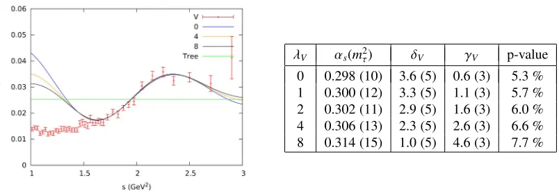
λV αs(m2τ) δV γV p-value 0 0.298 (10) 3.6 (5) 0.6 (3) 5.3 % 1 0.300 (12) 3.3 (5) 1.1 (3) 5.7 % 2 0.302 (11) 2.9 (5) 1.6 (3) 6.0 % 4 0.306 (13) 2.3 (5) 2.6 (3) 6.6 % 8 0.314 (15) 1.0 (5) 4.6 (3) 7.7 %

Figure 4.Vector spectral functionρ_V(s), fitted with the ansatz (14) for different values ofλV, compared with the

data points. The right table shows a representative subset of the fitted parameters with FOPT [30].

Instead of using clean moments where duality violations are suppressed, some works focus on observables more sensitive to these uncontrollable effects [36], modelling them with an ansatz for ∆ρDV

J (s) which is fitted to the measured spectral functions. Since the OPE is not valid on the physical cut, one loses theoretical control and gets at best an effective model description with unclear relation with QCD. Let us consider the slightly generalized ansatz (in GeV units)

∆ρDV J (s) = s

λJ _e−(δJ+γJs) _{sin (}α

J+βJs), s>sˆ0, (14)

which forλJ = 0 coincides with the model assumed in Ref. [36]. The combination of a dumping exponential with an oscillatory function is expected to describe the fall-offof duality violations at very high energies, but this functional form is completely ad-hoc and difficult to justify at low energies.

Since there are far too many parameters to be fitted to a highly-correlated data set, Ref. [36] con-centrates in the momentA(0_V,0)(s0) which is very exposed to violations of duality (ω(x)=1) and does

not receive OPE corrections (owing to the tail of thea1 resonance, the axial channel is not very

use-ful). The model parameters andαsare determined fitting thes0dependence fors0 ≥sˆ0=1.55 GeV2.

This choice has the largest, but still too small, p-value and gives the smallestαs. However, the p-value falls dramatically when one moves from this point, becoming worse at higher ˆs0 values where the

model should work better. The extracted value ofαsis very unstable under small modifications of the fit procedure and the fitted ansatz strongly deviates from the data as soon as one moves from the fitted region. This is illustrated in figure 4 which shows the results of this exercise with FOPT, for different values of the powerλVand ˆs0=1.55 GeV2. The actual uncertainties are much larger than the quoted

fit errors; varying ˆs0in the range [1.15,1.75] GeV2, withλV =0, induces 3σfluctuations ofαs(m2τ). All models reproduce wellρ_V(s) in the fitted region (s ≥1.55 GeV2_{), but they fail badly below}

4.3 Updated determination ofαs(m_τ)

The results shown in table 1 are based on solid theoretical principles (thes0-dependence extraction

as-sumes, however, local duality) and exhibit a good stability under small variations of the fit procedures. The overall agreement among determinations extracted under very different assumptions shows their reliability and even indicates that the uncertainties are probably too conservative. Averaging the five determinations, but keeping the smaller uncertainties to account for the large correlations, one finds

α(nf=3)

s (m2τ)CIPT = 0.335±0.013, α

(nf=3)

s (m2τ)FOPT = 0.320±0.012. (15)

The same results are obtained irrespective or whether one includes or not in the average the determi-nation from thes0dependence of the moments. Averaging the CIPT and FOPT “averages” in table 1,

one finally gets

α(nf=3)

s (m2τ) = 0.328±0.013. (16)

These results nicely agree with the value of the strong coupling extracted fromRτ[37]. After evolution up to the scaleMZ, the strong coupling decreases to

α(nf=5)

s (MZ2) = 0.1197±0.0015, (17)

in excellent agreement with the direct measurement at theZpeak in Eq. (9). The comparison of these two determinations, graphically shown in the right panel of figure 1, provides a beautiful test of the predicted QCD running;i.e., a very significant experimental verification of asymptotic freedom:

α(nf=5) s (MZ2)

_τ−α

(nf=5) s (MZ2)

_Z = 0.0001±0.0015τ±0.0030Z. (18)

Improvements on the determination ofαs(m2τ) from τdecay data would require high-precision measurements of the spectral functions, specially in the higher kinematically-allowed energy bins. Both higher statistics and a good control of experimental systematics are needed, which could be possible at the forthcoming Belle-II experiment. On the theoretical side, one needs an improved understanding of higher-order perturbative corrections.

5 World average value of

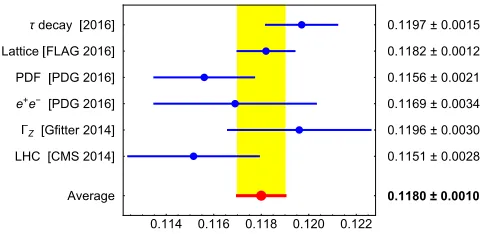
α

Figure 5 compares the N3LO determinations ofαs(M_Z2) fromZandτdecays with other precise mea-surements of the strong coupling. Following the PDG criteria [2], only those determinations which are at least of NNLO are taken into account. This includes several event-shape analyses in hadronic final states ofe+e−annihilations, and studies of parton distribution functions from deep inelastic scattering and hadron collider data. The numbers quoted in the figure correspond in both cases to the recent PDG compilation [2].

The PDG includes also in the average the CMS determination from thett¯production cross section at √s=7 TeV,αs(M2Z)=0.1151+

0.0028

−0.0027[38], which requires as input a value of the top quark mass

(eitherαsor mt are fitted to the data, but not both). Although there are more recent measurements of this cross section from ATLAS and CMS, at √s =7,8 and 13 TeV, none of them quotes further determinations ofαs. Applying the same procedure, these measurements would imply larger values ofαs(M_Z2) than the one of Ref. [38], which is nevertheless included in the average.

0.114 0.116 0.118 0.120 0.122

τdecay 2016]

Lattice FLAG 2016]

PDF PDG 2016]

e+e- [PDG 2016]

Z[Gfitter 2014]

LHC[CMS 2014]

Average

0.1197±0.0015

0.1182±0.0012

0.1156±0.0021

0.1169±0.0034

0.1196±0.0030

0.1151±0.0028

0.1180_±0.0010

Figure 5.Summary of the most precise determinations ofαs(M2Z).

expansions in powers of the strong coupling. The present situation has been recently summarized by the FLAG working group [39] which quotes the lattice world-average shown in figure 5.

The different determinations in figure 5 are in good agreement, within their quoted errors. From these results, one obtains the final world average value

αs(MZ2) = 0.1180±0.0010. (19)

This number is very close to the 2016 PDG average (0.1181±0.0011), which does not yet include the most recentτdecay and lattice results. The central value has been directly obtained as the weighted average of the six input determinations, while the error has been enlarged applying the PDG pre-scription, i.e., adjusting all individual uncertainties by a common factor such that χ2/dof equals unity. Removing the CMS determination would slightly increase the central value, giving as aver-ageαs(MZ2) =0.1183±0.0011. The overall uncertainty is largely determined by the precise lattice result.

Acknowledgements

I would like to thank Antonio Rodríguez Sánchez for a very enjoyable collaboration. This work has been sup-ported in part by the Spanish Government and ERDF funds from the EU Commission [Grant FPA2014-53631-C2-1-P], by the Spanish Centro de Excelencia Severo Ochoa Programme [Grant SEV-2014-0398] and by the Generalitat Valenciana [Grant PrometeoII/2013/007].

References

[1] C. Patrignaniet al.[Particle Data Group Collaboration], Chin. Phys. C40, no. 10, 100001 (2016). [2] S. Bethke, G. Dissertori and G. P. Salam, in [1], p. 132.

[3] D. d’Enterria et al., Proceedings “High-Precision αs Measurements from LHC to FCC-ee” (Geneva, Switzerland, October 2-13, 2015), arXiv:1512.05194 [hep-ph].

[4] A. Pich, PoS ConfinementX, 022 (2012) [arXiv:1303.2262 [hep-ph]].

[5] S. Bethke, Nucl. Phys. Proc. Suppl.234, 229 (2013) [arXiv:1210.0325 [hep-ex]].

[6] S. Bethkeet al., Proceedings “Workshop on Precision Measurements ofαs” (Munich, Germany, February 9-11, 2011), arXiv:1110.0016 [hep-ph].

[8] T. Lutheet al., JHEP1607, 127 (2016) [arXiv:1606.08662 [hep-ph]].

[9] T. van Ritbergen, J. A. M. Vermaseren and S. A. Larin, Phys. Lett. B400, 379 (1997) [hep-ph/9701390].

[10] M. Czakon, Nucl. Phys. B710, 485 (2005) [hep-ph/0411261].

[11] Y. Schroder and M. Steinhauser, JHEP0601, 051 (2006) [hep-ph/0512058].

[12] K. G. Chetyrkin, J. H. Kuhn and C. Sturm, Nucl. Phys. B744, 121 (2006) [hep-ph/0512060]. [13] P. A. Baikov, K. G. Chetyrkin and J. H. Kuhn, Phys. Rev. Lett. 101, 012002 (2008)

[arXiv:0801.1821 [hep-ph]].

[14] S. G. Gorishnii, A. L. Kataev and S. A. Larin, Phys. Lett. B259, 144 (1991).

[15] L. R. Surguladze and M. A. Samuel, Phys. Rev. Lett.66, 560 (1991) Erratum: [Phys. Rev. Lett. 66, 2416 (1991)].

[16] P. A. Baikov, K. G. Chetyrkin, J. H. Kuhn and J. Rittinger, Phys. Rev. Lett.108, 222003 (2012) [arXiv:1201.5804 [hep-ph]]; Phys. Lett. B714, 62 (2012) [arXiv:1206.1288 [hep-ph]].

[17] K. G. Chetyrkin, J. H. Kuhn and A. Kwiatkowski, Phys. Rept. 277, 189 (1996) [hep-ph/9503396].

[18] K. G. Chetyrkin, R. V. Harlander and J. H. Kuhn, Nucl. Phys. B586, 56 (2000) Erratum: [Nucl. Phys. B634, 413 (2002)] [hep-ph/0005139].

[19] M. Baaket al.[Gfitter Group Collaboration], Eur. Phys. J. C74, 3046 (2014) [arXiv:1407.3792 [hep-ph]].

[20] S. Narison and A. Pich, Phys. Lett. B211, 183 (1988).

[21] E. Braaten, Phys. Rev. Lett.60, 1606 (1988); Phys. Rev. D39, 1458 (1989). [22] E. Braaten, S. Narison and A. Pich, Nucl. Phys. B373, 581 (1992).

[23] W. J. Marciano and A. Sirlin, Phys. Rev. Lett.61, 1815 (1988). [24] E. Braaten and C. S. Li, Phys. Rev. D42, 3888 (1990). [25] J. Erler, Rev. Mex. Fis.50, 200 (2004) [hep-ph/0211345].

[26] M. Davieret al., Eur. Phys. J. C74, no. 3, 2803 (2014) [arXiv:1312.1501 [hep-ex]]. [27] F. Le Diberder and A. Pich, Phys. Lett. B289, 165 (1992).

[28] F. Le Diberder and A. Pich, Phys. Lett. B286, 147 (1992).

[29] A. A. Pivovarov, Z. Phys. C53, 461 (1992) [Sov. J. Nucl. Phys.54, 676 (1991)] [Yad. Fiz.54, 1114 (1991)] [hep-ph/0302003].

[30] A. Pich and A. Rodríguez-Sánchez, Phys. Rev. D94, no. 3, 034027 (2016) [arXiv:1605.06830 [hep-ph]]; Mod. Phys. Lett. A31, no. 30, 1630032 (2016) [arXiv:1606.07764 [hep-ph]].

[31] A. Pich, arXiv:1107.1123 [hep-ph].

[32] O. Cata, M. Golterman and S. Peris, Phys. Rev. D77, 093006 (2008) [arXiv:0803.0246 [hep-ph]].

[33] B. Chibisovet al., Int. J. Mod. Phys. A12, 2075 (1997) [hep-ph/9605465].

[34] M. González-Alonso, A. Pich and J. Prades, Phys. Rev. D81, 074007 (2010) [arXiv:1001.2269 [hep-ph]].

[35] M. González-Alonso, A. Pich and A. Rodríguez-Sánchez, Phys. Rev. D94, no. 1, 014017 (2016) [arXiv:1602.06112 [hep-ph]].

[36] D. Boitoet al., Phys. Rev. D91, no. 3, 034003 (2015) [arXiv:1410.3528 [hep-ph]]. [37] A. Pich, Prog. Part. Nucl. Phys.75, 41 (2014) [arXiv:1310.7922 [hep-ph]].

[38] S. Chatrchyanet al.[CMS Collaboration], Phys. Lett. B728, 496 (2014) Erratum: [Phys. Lett. B738, 526 (2014)] [arXiv:1307.1907 [hep-ex]].