824
Projection Based Data Depth Procedure with
Application in Discriminant Analysis
Muthukrishnan R1, Vadivel M2, Ramkumar N3
Department of Statistics, Bharathiar University, Coimbatore, Tamil Nadu, India1,2,3 Email: [email protected]1 ,[email protected]2 ,[email protected]3
Abstract- Projection depth and its associated estimators, namely, Stahel-Donoho (S-D) estimator, Projection Trimmed Mean (PTM), Projection depth Contours (PC) and Projection Median (PM) have been studied in bivariate data. An attempt has been made to compute projection depth and its associated estimators by using the pair of location and scale estimator (Mean, Standard Deviation (SD)), (Median, Median Absolute Deviation (MAD)), and (Median, Qn).The efficiency of these estimators is carried out by computing average
misclassification error in discriminant analysis by using the projection depth based Stahel-Donohoestimator under real and simulating environment. The study concluded that (Median, MAD) and (Median, Qn) based
projection depth estimators performs well when compared with (Mean, SD).
Index Terms-Projection depth and its associated estimators; Robust discrimination analysis.
1. INTRODUCTION
Data depth is a concept which plays an important role in many notable fields of statistics,namely; data exploration, ordering, asymptotic distributions and robust estimation(Liu et al. 1999). The essence of the depth function in multivariate analyses is to measure degree of centrality of a point relative to a data set or to a probability distribution. Many robust procedures have been developed to compute the data depth. The data depth based approach has been received much attention now-a-days. Numerous depth notations have been proposed during the last few decades, namely,half space depth (Tukey 1975), simplicial depth (Liu 1990), regression depth (Rousseeuw and Hubert 1999) and projection depth (Liu 1992; Zuo and Serfling 2000; Zuo 2003).
The Projection Depth(PD) is very favorable to the robust statistics when compared with the other depth notations.It is due to the reason that all the desirable properties of the general statistical depth function defined in Zuo and Serfling (2000), namely, affine invariance, maximality at center, monotonicity relative to deepest point, and vanishing at infinity are satisfied by the PD.
The main objective of this paper is to estimate the associated estimators such as Stahel-Donohoestimator, projection trimmed mean, projection depth contours and projection median for bivariate data based on various pair of projection depth procedures.Further, the performance of the pairs has been studied under various levels of contaminations with the help of
Stahel-Donohoestimator, by computing average
misclassification probabilities in the context of robust
linear discriminant analysis in Hubert and Van Driessen (2014).
The rest of the paper is organized as follows. Section 2 describes the methodology of projection depth and its associated estimators. Section 3 discussesrobust linear discriminant analysis. Section 4 examines the performance and critically compares the three pairs of projection depth procedures. Section 5 presents results obtained in real and simulation studyin the context of robust discriminate analysis.The paper ends with conclusion in the last section.
2. PROJECTION DEPTH AND ITS ASSOCIATED ESTIMATORS
Zuo (2003) introduced a Projection-based depth functions, which has the highest breakdown point among all the existing affine equivariant multivariate location estimators and associated medians. It can induce a lot of favorable estimators, such as Stahel-Donohoestimator and depth weighted means for multivariate data (Zuo et al. 2004; Zuo 2006).Further, Zuo (2006) studied multidimensional trimming based on projection depth. Exact computation of bivariate projection depth and Stahel-Donoho estimator, with a proper choice of
,
are formulated and studied by Zuo and Lai (2011). Liu and Zuo (2014) studied computational aspects of projection depth and its associated estimators.The brief description of theory of projection depth is as follows.825 a point
x
R
with respect to the distributionfunctionF of Xdefinedby (Liu 1992, Zuo 2003).
, ) , ( 1 1 ) , ( F x O F x PD where,
,
,
,
sup
)
,
(
1F
x
u
Q
F
x
O
u
(1)where,
u
F
F
u u T x F x u
Q , , / and Fuis the
distribution ofuTx. If
u
Tx
(
F
u)
F
u
0
,then define
Q
u
,
x
,
F
0
, which denotes the projection of xonto the unit vector u. Note that the most popular outlying function has the robust choice of µ andσ be theMedian and MAD. Here, the pair (med, Qn), where med and Qnis considered as locationand scale estimator of (µ(F), σ(F)) for a given sample Xn = {X1, X2,…,Xn} from X.Let Fn be the
corresponding distribution, then the projection depth and its associated estimators depend on the robust choice of (Med, Qn), Q(x,u,X
n
) in (1) with respect to u.
x
X
Q
u
x
X
Q
nu
n
sup
,
,
,
1
, (2) The outlying function is defined as
,
,
,
X
u
Q
X
u
Med
x
u
X
x
u
Q
n T n n T Tn
(3) WhereuTdenotes the projection ofxonto the unit vector
u and
u
TX
n
u
TX
1,
u
TX
2,...,
u
TX
n
. LetX(1) ≤ X (2) ≤ … ≤ X(n) denote the order statistics
corresponding to the univariate random variablesZn.
,
2
)
(
X
X
1/2X
2 /2Med
n
n
n
;
,
)
(
j
i
X j
X i
d
X
Q
k
n
n
wheredis a constant factor and
/
4
,
2
2
h
n
k
1
2
n
h
is roughly half the number ofobservations. That is,
2
n
is the interpoint distances
ofkth order statistics.
The main function of the projection depth is to be responsible for a center-outward ordering for the bivariate data. Based on this ordering, one can make the projection depth contours, which can provide us with a bivariate data of the quantile of an underlying distribution (Halin et al. 2010).
It’s defined as
:
(
,
)
,
)
,
(
F
x
R
PD
x
F
PR
P(4)
where
0
*sup
PD
(
x
,
F
)
R
P x
with αthProjection depth Region (DR).Then the corresponding αth
Projection Depth Contour can be distinct as the boundary ofPDR (α,F)under some conditions (Zuo 2003) is given by
:
(
,
)
.
)
,
(
F
x
R
PD
x
F
PC
P(5) The innermost depth contour, which is a singleton in many situations, is the Projection depth Median (PM) of Zuo (2003)
.
)
,
(
)
(
F
PC
*F
PM
Based on the projection depth regionPR (α, F),one can define theαth Projectiondepth Trimmed Mean (PTM), (Zuo (2006)) as
(
,
(
))
,
,
)
,
(
) , ( 1 , 1
F PR F PRdx
F
F
x
PD
dx
F
F
x
PD
x
F
PTM
w
w
(6) wherew1(.)is a suitable (bound) weight function on [0,1]. PTM is highly robustness and efficiency α=0 and the famous degenerates PTM into the Stahel-Donoho location estimators (Stahel 1981; Donoho and Gasko 1992), i.e.theProjection Weighted Mean (PWM) and Projection Weighted Scatter (PWS)
,
,
,
1 1dx
F
F
x
PD
w
dx
F
F
x
PD
w
x
F
PWM
(7)
,
,
,
2 2
dx
F
F
x
PD
dx
F
F
x
PD
F
PWM
x
F
PWS
w
w
F
PWM
x
(8)wherePWM(F) and PWS(F)is the aforementioned Stahel-Donoho location and scatter estimator,w2(.)
denotes the weight function on [0, 1] based on projection depth outlying function (µ(F),Qn(F))as
826 associated estimators such asPTM (F), PWM
(F)andPWS (F)to be well defined, certain monotony conditions are required as follows:
(
,
)
0
,
w
iPD
x
F
F
dx
x
iw
iPD
x
,
F
F
dx
,
i
1
,
2
.
with a finite sample
X
n
X
1,
X
2,...,
X
n
from XandFn be the corresponding empirical distribution of F
based onXn. By simply replacing F byFnin projection depth and its related estimators can obtain their sample version.
3. ROBUST DISCRIMINANT ANALYSIS
Let p be the variable with nobservations that are sampled froml different populations π1,…,πl. The
discriminant analysis settingis in the membership of each observation with respect to the populations, i.e., the data points intolgroups with n1,n2,…,nl
observations. Trivially,
l
j j
n
n
1
.
Therefore, thenthe observations by
x
ij;
j
1
,...,
l
;
i
1
,...,
n
j
.
Based on the initial estimates µj,0 and Sj,0 are computed
for each observation xijof group jand its (preliminary)
robust distance is given by
The assign weight 1 to xiif
. 2
975 . 0 , 0
ij
RD
The reweighted projection depth estimator for group j is then obtained as the medianPWMjand the
scatter matrixPWSjof those observations of group j
with weight 1. It is shown that this reweighting step increases the finite-sample efficiency of the projection depth estimator considerably, whereas the breakdown value remains the same. These robust estimates of location and scatter now allow us to flag the outliers in the data, and to obtain more robust estimates of the membership probabilities. First compute the robust distance for each observation xijfrom group j,
,
0
1
,0
.
0
,
x
PWM
PWS
PWM j
xij
RD
j ij jt
ij
One can consideran observation xijis an outlier if and
only if
.
2 975 . 0 , p ij
RD
Further, the projection depth estimatesPWMjand
PWSjare obtained for each group, and then the
individual covariance matrixes are pooled together for further computation.
Letnjdenote the number of non-outliers in group j, and
l
j j
n
n
1
, then the robustly estimate the
membership probabilities as
.
n
n
P
jR
jNote that the usual estimates implicitly assume that all the observations have been correctly assigned to their group. It is however also possible that typographical or other error has occurred when the group numbers were recorded. The observations that are accidently put in the wrong group will then probably show up as outliers in that group, and so they will not influence the estimates of the membership probabilities. Of course, if one is sure that this kind of error is not present in the data, one can still use the relative frequencies based on all the observations.
4. RESULTS AND DISCUSSION
4.1. Simulation (Computing Projection Depth values)
A simulation study is performed to compare the efficiency of the various notions of projection depth procedures. To illustrate this 25 sample points are simulated from multivariate normal distribution with the mean vector µ= (1,1) and the covariance matrixI2
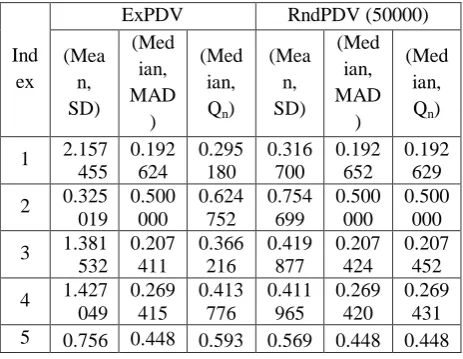
The obtained finite number of optimal direction vectors under the exact projection depth values of the sample points with respect to the data cloud χn
is reported in Table 1 and is given in Appendix. For the sake of comparison, it is also computed the approximate projection depth values based on 5 × 10⁴ random direction vectors. It is observed from the table, the exact projection depth values are almost greater than the random projection depth values by considering all the pairs. Further it is noted that the exact projection depth values is greater than the random projection depth values produced by the pair (Mean, SD). It is concluded that the pairs (Median, MAD) and (Median, Qn) produces similar
depth values under exact and random projections. The projection depth size plots under exact and random projections are displayed in the figure 1.It is noted that the size of the plotted points is increases when the depth values increases. That is, the plotted pointsare in bigger size when the depth value is large. Again, thedepth central points are largerelative to those on the skirts. This is a confirmation that the
,
0
1
.
0
ij
j,0j t
ij
xij
j
S
x
827 projection depth provides a center-outward ordering
for the given data cloud.
Mean,SD Median, MAD Median, Qn
[image:4.595.304.589.594.728.2]Exact projectio ns Random projectio ns
Figure 1Projection Depth-Size Plots
4.2.Simulation (Computing Projection-based depth and its associated estimators)
In order to compare the projection-based depth and its associated estimators, 100 datapoints were generated from the normal distribution with the mean vector µ=(1, 1) and covariance matrix
1 0 0 1 . Further, the location and scale estimates for the generated data is computed which are as follows:µ = (1.1271,1.0392),Med = (1.1476,1.0706) and
1041 . 1 1097 . 0 1097 . 0 0481 . 1
which are mean, median and covariance respectively. The estimated Projection based Median, Weighted Median and Trimmed Median under the three pairs (Mean, SD), (Median, MAD) and (Median, Qn) are summarized in table 2
and 3.
Further, the study was extended with contamination. The data generated with µ = (-4, -4), ∑ = 4IP, and the level of contamination 5%, 10% and
15% were considered, and then the same experiment was performed. For the contaminated data, the computed location and scatter values mean, median and covariance are µ = 0.5293, -0.7022), med =
(-0.0333,-0.3286) and
2617 . 4 5105 . 2 5105 . 2 1224 . 4
respectively.The estimated Projection based Median, Weighted Median and Trimmed Median under the three pairs (Mean, SD), (Median, MAD) and (Median, Qn) are also summarized in table 2 and 3.
Table2Estimated Projection Depth Location Estimators (with/without contamination)
Error Estimat ors
Projection Depth Procedures
(Mean, SD) (Median, MAD) (Median, Qn)
0.00
PM (1.1271, 1.0392) (1.0807, 1.0724) (1.0830, 1.0661) PWM (1.1326, 1.0458) (1.1402, 1.0538) (1.1326, 1.0458) PTM (1.1463, 1.0520) (1.1329, 1.0589) (1.1463, 1.0520)
0.05
PM (0.9082,0.6899) (1.0198,0.8114) (1.0211,0.8138) PWM (1.0291,0.8099) (1.0458,0.8360) (1.0501,0.8346) PTM (1.0893,0.8661) (1.1041,0.8980) (1.2106,0.8844)
0.10
PM (1.1271,1.0392) (1.0825,1.0593) (1.0830,1.0661) PWM (1.1359,1.0366) (1.1322,1.0412) (1.1325,1.0457) PTM (1.1499,1.0432) (1.1261,1.0388) (1.1464,1.0519)
0.15
PM (0.3484,0.2410) (0.7592,0.5882) (0.8110,0.6337) PWM (0.6903,0.4843) (0.7928,0.5825) (0.8904,0.6602) PTM (0.8037,0.5591) (1.0345,0.7809) (1.1385,0.8555)
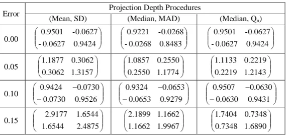
Table3Estimated Projection depth weighted Scatter Estimators (with/withoutcontamination)
Error Projection Depth Procedures
(Mean, SD) (Median, MAD) (Median, Qn)
0.00
0.9424 0.0627 --0.0627 0.9501 0.8483 0.0268 --0.0268 0.9221 0.9424 0.0627 --0.0627 0.9501
0.05
3157 . 1 3062 . 0 3062 . 0 1877 . 1 1774 . 1 2550 . 0 2550 . 0 0857 . 1 2143 . 1 2219 . 0 2219 . 0 1133 . 1
0.10
9526 . 0 0730 . 0 0730 . 0 9424 . 0 9279 . 0 0653 . 0 0653 . 0 9324 . 0 9431 . 0 0630 . 0 0630 . 0 9507 . 0
0.15
4875 . 2 6544 . 1 6544 . 1 2.9177 9967 . 1 1662 . 1 1662 . 1 1899 . 2 6890 . 1 7348 . 0 7348 . 0 7404 . 1
828 actual value under the three pair of estimators when
there is no contamination. Further, it is noted that the pair (Median, Qn) can tolerate certain amount of
contamination, specifically, one can see that the contamination level is 15%, the results get affected under the pairs (Mean, SD) and (Median, MAD) but not in the case of (Median, Qn). It is concluded that,
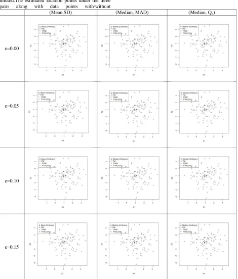
the impact of the outliers on(Median, Qn) are very limited.The estimated location points under the three pairs along with data points with/without
contaminations are displayed in the form of scatter plots in Figure.2. Figures reveal that the ordinary
mean is placed outside the bulk of the data points by a few outliers; while other projection depth based location estimators are positioned among the majority of the data.
(Mean,SD) (Median, MAD) (Median, Qn)
e=0.00
e=0.05
e=0.10
[image:5.595.73.544.196.748.2]e=0.15
829 The location and scatter estimators confirm high
robustness of projection depth and its associated estimators (Zuo 2003, 2006).It is worthy to note that, during the computation of PWM, PTM and PWS; weight functionswi(.), i =1,2,used here as suggested by
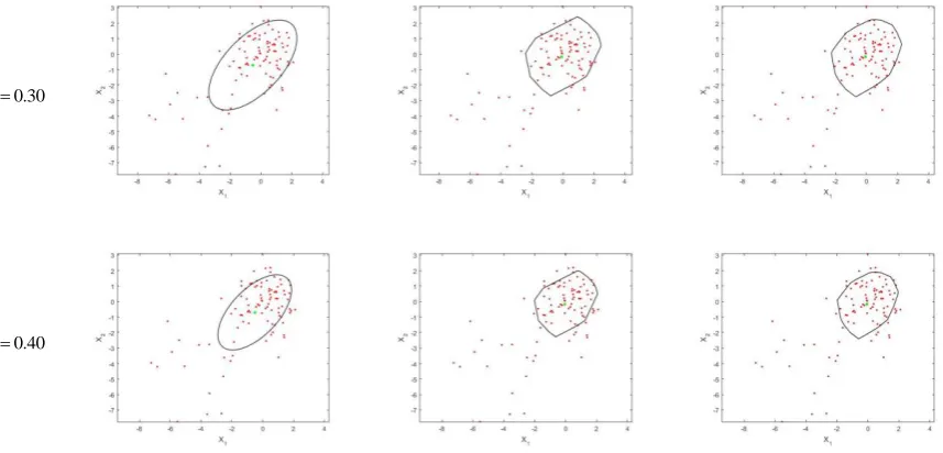
Zuo and Cui (2005). Further the projection depth contours applied to various projection-based depth procedures under various level of contaminations are display in figure 3 and is given in Appendix. The contours indicate a similarity in the structures of the projection depth procedures (Median, MAD) and (Median, Qn) which are both unlike the results of the
procedure (Mean, SD).
5. APPLICATIONS IN DISCRIMINANT ANALYSIS
5.1.Real data
This section presents the performance of projection depth based SDE in robust linear discriminant analysis by computing misclassification probabilities with three pairs of location and scatter approach. It is considered a data set with two groups (Johnson and Wichern (2009)). The data description is as follows: Two different groups: π1 is ridingmover
owners and π2 is without riding movers to identify the
best sales prospects. The owners or non-owners on the basis ofthe variables x1(income), x2(lot size), random
sampleofsize n1(=12) current owners and n2(=12)
current non-owners respectively. Discriminant analysis for these two groups is performed and computed misclassification probabilities under various
[image:6.595.69.535.490.579.2]projection depths based approaches and is given in table 4.
Table 4Computed misclassification probabilities under various projection depth
Procedures Misclassification Probabilities
π1 π2 Average
(Mean, SD) 0.1667 0.1667 0.1667
(Median, MAD) 0.2083 0.2083 0.2083
(Median, Qn) 0.1667 0.1667 0.1667
The estimated average misclassification probabilities are almost same except the procedure(Median, MAD).
5.2.Simulation study
This section presents the results obtained under various projection depth based approaches under simulating environment with/without contaminations (Location and Scale). In this context, two groups (g=2) with two variables (p=2) are considered to simulate the data. The data were generated under thenormal distribution which hasthe covariance matrices ∑1=IP and ∑2= 2IP with means µ1=
(1, 1) and µ2= (5, 5)under sample sizes of 50 and 100.
The various levels of contaminations such as 5%, 10%, 15%, 20%, 25%, 30%, 35% and 40% were considered in all cases. The obtained results with the contamination levels 0%, 5%, 10% and 15% are same and the results based on the remaining contaminations are displayed in the table 5.
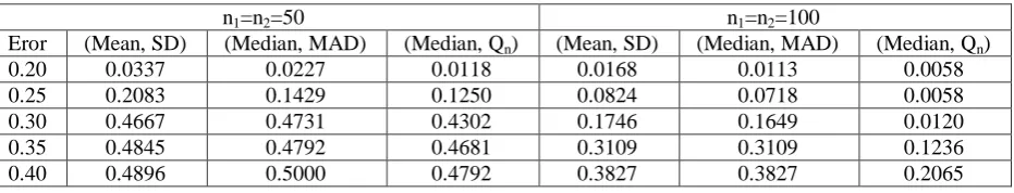
Table5Computed misclassification probabilities under various projection depths with contaminations
n1=n2=50 n1=n2=100
Eror (Mean, SD) (Median, MAD) (Median, Qn) (Mean, SD) (Median, MAD) (Median, Qn)
0.20 0.0337 0.0227 0.0118 0.0168 0.0113 0.0058
0.25 0.2083 0.1429 0.1250 0.0824 0.0718 0.0058
0.30 0.4667 0.4731 0.4302 0.1746 0.1649 0.0120
0.35 0.4845 0.4792 0.4681 0.3109 0.3109 0.1236
0.40 0.4896 0.5000 0.4792 0.3827 0.3827 0.2065
On comparing the average probability of misclassification values in the above table, it is evident that the procedures (Median, MAD) and (Median, Qn) produces less when compared with
(Mean,SD). Also, it is observed that when sample size increases the misclassification probabilities decreased under all the procedures. It is concluded that the procedure (Median, Qn) performs better than the other
two procedures. It shows that it is superior to the other two procedures when the level of contamination increases.
6. CONCLUSION
Location and scatter estimator play vital role in almost all statistical data analyses. The conventional estimates, sample mean vector and covariance matrix are very sensitive when the outlying observations in the data. In order to obtain the reliable location and scatter estimate, data depth approaches attract the researchers now-a-days. This paper proposes a projection based data depth approach to compute location and scatter estimate, namely (Median, Qn).
830 (Median, MAD). The simulation study shows that the
projection depth based on the mean and standard deviation fails to produce reliable results when compared with the other projection depth procedures. It is noted that (Median, MAD) and (Median, Qn)
performs well over the (Mean, SD). The study concluded that the proposed projection depth procedure (Median,Qn)shows that its superiority over
the other procedures (Mean, SD) and (Median, MAD), in the context of tolerance level of contaminations and misclassification rate.
Acknowledgement
This research work was funded by the Rajiv Gandhi National Fellowship (RGNF) programme, UGC, New Delhi and carried out at Department of Statistics, Bharathiar University, Tamil Nadu and India.
REFERENCES
1. Donoho, D. L., and Gasko, M. (1992). Breakdown properties of location estimates based on halfspace depth and projected outlyingness. .
The Annals of Statistics. 20, 1803–1827.
2. Halin, M., Paindaveine, D., and Siman, M. (2010). Multivariate quantiles and multiple-output regression quantiles: From L1 optimization to halfspace depth. The Annals of Statistics, 38(2), 635-669.
3. Hu, Y., Li, Q., Wang, Y., and Wu, Y. (2012). Rayleigh projection depth. Computational Statistics, 27, 523-530.
4. Hubert, M. and Van Driessen, K. (2004). Fast and Robust Discriminant Analysis. Computaional Statistics & Data Analysis, 45,301,320.
5. Johnson, R.A., and Wichern, D.W (2009). Applied multivariate analysis, 5th ed. Prentice Hall, Englewood Cliffs, New Jersey.
6. Liu, R.Y. (1990). On a notion of data depth based on random simplices. The Annals of Statistics, 18, 191-219.
7. Liu, R.Y. (1992). Data depth and multivariate rank test. In: L1- Statistical Analysis and Related Methods, 279-294. North-Holland, Amsterdam. 8. Liu, R.Y., Parelius, J.M., and Singh, K. (1999).
Multivariate analysis by data depth: Descriptive Statistics, Graphics and Inference. The Annals of Statistics, 27, 783-858.
9. Liu, X., and Zuo, Y. (2014). Computing projection depth and its associated estimators.
Stat.Comput., 24, 51-63.
10. Liu, X.H., Zuo, Y.J., Wang, Z.Z. (2011). Exactly computing bivariate projection depth contours and median. Preprint.
11. Rousseeuw, P.J., and Hubert, M. (1999). Regression depth. Journal of the American Statistical Association, 94, 388-433.
12. Stahel, W.A. (1981). Breakdown of covariance estimators. Research Report 31, 1029-1036. 13. Tukey, J.W. (1975). Mathematics and the
picturing of data. In: Proceedings of the International Congress of Mathematicians, pp. 523-531. Canadian Mathematical Congress, Montreal.
14. Zuo, Y. (2003). Projection-based depth functions and associated medians, The Annals of Statistics, 31, 1460-1490.
15. Zuo, Y., and Serfling, R. (2000). General notions of statistical depth function. The Annals of Statistics, 28, 461–482.
16. Zuo, Y.J. (2006). Multidimensional trimming based on projection depth. The Annals of Statistics, 34, 2211-2251.
17. Zuo, Y.J., and Lai, S.Y. (2011). Exact computation of bivariate projection depth and Stahel-Donoho estimator. Computational Statistics & Data Analysis, 55(3), 1173-1179. 18. Zuo, Y.J., and Cui, H.J. (2005). Depth weighted
scatter estimators. The Annals of Statistics, 33, 381-413.
19. Zuo, Y.J., Cui, H.J., He, X.M. (2004). On the Stahel-Donoho estimators and depth – weighted means for multivariate data. The Annals of Statistics, 32(1), 189-218.
[image:7.595.301.533.591.770.2]Appendix A.
Table 1 Computed Exact and Random Projection Depth Values
Ind ex
ExPDV RndPDV (50000)
(Mea n, SD)
(Med ian, MAD
)
(Med ian, Qn)
(Mea n, SD)
(Med ian, MAD )
(Med ian, Qn)
1 2.157 455
0.192 624
0.295 180
0.316 700
0.192 652
0.192 629 2 0.325
019 0.500
000
0.624 752
0.754 699
0.500 000
0.500 000 3 1.381
532 0.207
411
0.366 216
0.419 877
0.207 424
0.207 452 4 1.427
049 0.269
415
0.413 776
0.411 965
0.269 420
0.269 431
831
764 481 490 181 493 500
6 1.110 552 0.232 646 0.403 110 0.473 809 0.232 665 0.232 688 7 0.578
716 0.468 108 0.627 823 0.633 426 0.468 113 0.468 110 8 2.088
440 0.210 192 0.330 685 0.323 738 0.210 192 0.210 194 9 1.365
669 0.266 899 0.389 780 0.422 712 0.266 935 0.266 904 10 1.849
254 0.231 068 0.370 514 0.350 968 0.231 075 0.231 072 11 0.711
800 0.441 931 0.577 139 0.584 118 0.441 932 0.441 936 12 0.968
409 0.375 329 0.507 785 0.508 010 0.375 332 0.375 342 13 0.664
505 0.431 879 0.595 967 0.600 772 0.431 887 0.431 883 14 0.654
543 0.323 455 0.512 907 0.604 381 0.323 470 0.323 503 15 2.226
154 0.162 738 0.287 439 0.309 962 0.162 756 0.162 757
16 1.894 023 0.159 594 0.296 955 0.345 536 0.159 607 0.159 621 17 1.177
729 0.316 469 0.442 848 0.459 100 0.316 471 0.316 484 18 0.438
135 0.523 140 0.677 843 0.695 193 0.523 145 0.523 143 19 1.925
905 0.211 008 0.364 037 0.341 707 0.211 022 0.211 023 20 1.534
453 0.245 126 0.363 464 0.394 543 0.245 160 0.245 131 21 1.860
163 0.165 077 0.306 217 0.349 630 0.165 093 0.165 103 22 1.083
207 0.302 623 0.431 504 0.480 021 0.302 626 0.302 646 23 0.647
058 0.395 693 0.534 016 0.607 130 0.395 696 0.395 718 24 1.874
344 0.228 289 0.355 446 0.347 905 0.228 299 0.228 294 25 0.657
895 0.500 000 0.637 665 0.603 174 0.500 000 0.500 000
(Mean,SD) (Median, MAD) (Median, Qn)
832 30
. 0
40 . 0
[image:9.595.89.518.115.321.2]