Sentence Ordering based on Cluster Adjacency in Multi-Document
Summarization
Ji Donghong, Nie Yu
Institute for Infocomm Research
Singapore, 119613
{dhji, ynie}@i2r.a-star.edu.sg
ABSTRACT
In this paper, we propose a cluster-adjacency based method to order sentences for multi-document summarization tasks. Given a group of sentences to be organized into a summary, each sentence was mapped to a theme in source documents by a semi-supervised classification method, and adjacency of pairs of sentences is learned from source documents based on adjacency of clusters they belong to. Then the ordering of the summary sentences can be derived with the first sentence determined. Experiments and evaluations on DUC04 data show that this method gets better performance than other existing sentence ordering methods.
1.
Introduction
The issue of how to extract information from source documents is one main topic of summarization area. Being the last step of multi-document summarization tasks, sentence ordering attracts less attention up to now. But since a good summary should be fluent and readable to human being, sentence ordering which organizes texts into the final summary could not be ignored.
Sentence ordering is much harder for multi-document summarization than for single-document summarization (McKeown et al., 2001; Barzilay and Lapata, 2005). The main reason is that unlike single document, multi-documents don’t provide a natural order of texts to be the basis of sentence ordering judgment. This is more obvious for sentence extraction based summarization systems.
Majority ordering is one way of sentence ordering (McKeown et al., 2001; Barzilay et al., 2002). This method groups sentences in source documents into different themes or topics based on summary sentences to be ordered, and the order of summary sentences is determined based on the order of themes. The idea of this method is reasonable since the summary of multi-documents usually covers several topics in source documents to achieve representative, and the theme ordering can suggest sentence ordering somehow. However, there are two challenges for this method. One is how to cluster sentences into topics, and the other is how to order sentences belonging to the same topic. Barzilay et al. (2002) combined topic relatedness and chronological ordering together to order sentences. Besides chronological ordering,
sentences were also grouped into different themes and ordered by the order of themes learned from source documents. The results show that topic relatedness can help chronological ordering to improve the performance.
Probabilistic model was also used to order sentences. Lapata (2003) ordered sentences based on conditional probabilities of sentence pairs. The conditional probabilities of sentence pairs were learned from a training corpus. With conditional probability of each sentence pairs, the approximate optimal global ordering was achieved with a simple greedy algorithm. The conditional probability of a pair of sentences was calculated by conditional probability of feature pairs occurring in the two sentences. The experiment results show that it gets significant improvement compared with randomly sentence ranking.
Bollegala et al. (2005) combined chronological ordering, probabilistic ordering and topic relatedness ordering together. They used a machine learning approach to learn the way of combination of the three ordering methods. The combined system got better results than any of the three individual methods.
Nie et al. (2006) used adjacency of sentence pairs to order sentences. Instead of the probability of a sentence sequence used in probabilistic model, the adjacency model used adjacency value of sentence pairs to order sentences. Sentence adjacency is calculated based on adjacency of feature pairs within the sentence pairs. Adjacency between two sentences means how closely they should be put together in a set of summary sentences. Although there is no ordering information provided by sentence adjacency, an optimal ordering of summary sentences can be derived by use of adjacency information of all sentence pairs if the first sentence is properly selected.
information to limited number of individual features, which usually needs manual intervention.
The remainder of this paper is organized as follows. In section 2, we specify the motivation of this method. In section 3, we talk about the sentence classification using a semi-supervised method. In section 4, we discuss the procedure for sentence ordering. In section 5, we present experiments and evaluation. In section 6, we give the conclusion and future work.
2.
Motivation
Majority ordering assumes that sentences in the summary belong to different themes or topics, and the ordering of sentences in the summary can be determined by the occurring sequence of themes in source documents. In order to derive the order of themes, Barzilay et al. (2002) presented themes and their relations as a directed graph. In the graph, nodes denote themes; an edge from one node to another denotes the occurring of one theme before another in a source document, and the weight of an edge is set to be the frequency of the theme pair co-occurring in the texts. Each theme is given a weight that equals to the difference between its outgoing edges and incoming edges. By finding and removing a theme with the biggest weight in the graph recursively, an ordering of themes is determined.
Probabilistic ordering method treats the ordering as a task of finding the sentence sequence with the biggest probability (Lapata, 2003). For a sentence sequence T= S1, S2,…,Sn ,
suppose that the probability of any given sentence is determined only by its previous sentence, the probability of a sentence sequence can be generated based on the condition probabilities P(Si|Si-1) of all adjacent sentence pairs in the
sequence. The condition probability P(Si|Si-1) can be further
resolved as the product of condition probabilities of feature pairs P(fl|fm), where fl is the feature in Si, fm is the feature in
Si-1.
By finding the sentence with the biggest condition probability with the previous one recursively, an ordering of sentences is determined. A null sentence is normally introduced at the beginning of each source document to find the first sentence (Lapata, 2003).
Both majority ordering and probabilistic ordering determine text sequences in the summary based on those in the source documents. The intuition behind the idea is that the ordering of summary sentences tends to be consistent with those of document sentences. However, we notice that some important information might be lost in the process. Consider examples below:
Example 1: Source Document = ……ABA…… Example 2: Source Document 1 = ……AB…… Source Document 2 = ……BA……
Here A and B denote two themes. Let’s assume that A and B are both denoted by the summary sentences. In both examples, the frequency of A preceding B equals to that of B preceding A, thus no sequence preference could be learned
from the two examples, and we can only estimate a probability of 0.5 following one by another. With such estimation, the intuition that A and B shall be put adjacently although their ordering is not clear would be difficult to capture.
An adjacency based ordering (Nie et al., 2006) was proposed to capture such adjacency information between texts during sentence ordering. It uses adjacency of sentence pairs to order summary sentences. Adjacency between two sentences can be seen as how closely they should be put together in an output summary. In general, sentence adjacency is derived from that of feature pairs within sentences. Note that there is no clue to decide the sequence of two sentences purely based on their adjacency value. However, if the first sentence has been decided, the total sentence sequence can be derived according to the adjacency values by recursively selecting one having the biggest adjacency value with the most recently selected.
For adjacency based ordering, a problem is how to calculate the adjacency value between two sentences. For feature-adjacency based ordering, the sentence adjacency is calculated based on that of feature pairs within the two sentences. But a sentence may contain many single word features, and there may exist many noisy features, especially for longer sentences. To eliminate the impact of noisy features, one simple method is to select top n most adjacent feature pairs among the two sentences (Nie et al., 2006). However, the parameter heavily influences the performance, as shown in Table 1, where each row gives the result of a run with the same window range and different top n adjacent feature pairs.
Win_ range
τ( top-n=1)
τ( top-n=2)
τ(top -n=3)
τ( top-n=4)
τ( top-n=5)
τ( top-n=10)
2 0.184 0.213 0.253 0.262 0.261 0.224
3 0.251 0.252 0.273 0.274 0.257 0.213
4 0.201 0.253 0.268 0.316 0.272 0.248 Table 1. Feature-Adjacency Based Ordering
The heavy reliance on the manually pre-defined parameter is an obstacle for implementation of the feature-adjacency based ordering, since it’s hard to determine the most suitable value for the parameter across different tasks. More generally, the feature-adjacency method depends on limited number of individual features, which normally needs very strong feature selection techniques to be effective. To avoid the sensitivity to individual features, we propose a cluster-adjacency based sentence ordering. Although the clustering will also use individual features, the noisy ones would be lower weighted via appropriate weighting schemes.
adjacency, the setting of the parameter to remove noisy features is no more needed. In addition, we expect the clustering to determine the themes properly and reduce the affect of noisy features.
3. Sentence Clustering
Assume there are K summary sentences to be ordered, and there are N sentences in source documents, we cluster the N sentences into K clusters using a semi-supervised classification method, Label Propagation (Zhu and Ghahramani, 2003). The advantage of this method is that it can exploit the closeness between unlabeled data during classification, thus ensuring a better classification result even with very fewer labeled data. This is exactly the situation here, where each summary sentence can be seen as the only one labeled data for the class.
Following are some notations for the label propagation algorithm in sentence classification:
{rj} (1≤j≤K): the K summary sentences
{mj} (1≤j≤N): the N document sentences to be classified
X = {xi} (1≤i≤K+N) refers to the union set of the above
two categories of sentences, i.e. xi (1≤i≤K) represents the K
summary sentences, xi (K+1≤i≤K+N+1) represents the N
sentences to be classified. That is, the first K sentences are labeled sentences while the remaining N sentences are to be re-ranked. C = {cj} (1≤j≤K) denotes the class set of
sentences, each one in which is labeled by a summary sentence. Y0
∈
Hs×K (s=K+N) represents initial soft labels attached to each sentence, where Yij0= 1 if xi is cj and 0otherwise. Let YL0 be top l=K rows of Y0, which corresponds
to the labeled data, and YU0 be the remaining N rows, which
corresponds to the unlabeled data. Here, each row in YU0 is
initialized according to the similarity of a sentence with the summary sentences.
In the label propagation algorithm, the manifold structure in X is represented as a connected graph and the label information of any vertex in the graph is propagated to nearby vertices through weighted edges until the propagation process converges. Here, each vertex corresponds to a sentence, and the edge between any two sentences xi and xj is
weighted by wij to measure their similarity. Here wij is defined
as follows: wij = exp(-dij2/ σ 2) if i ≠ j and wii = 0 (1≤i,j≤l+u),
where dij is the distance between xi and xj, and σ is a scale to
control the transformation. In this paper, we set σ as the average distance between summary sentences. Moreover, the weight wij between two sentences xi and xj is transformed to a
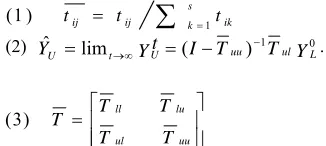
probability tij = P(j→i) =wij/(∑sk=1wkj), where tij is the
probability to propagate a label from sentence xj to sentence
xi. In principle, larger weights between two sentences mean
easy travel and similar labels between them according to the global consistency assumption applied in this algorithm. Finally, tij is normalized row by row as in (1), which is to
maintain the class probability interpretation of Y. The s × s matrix is denoted asTas in (1).
During the label propagation process, the label distribution of the labeled data is clamped in each loop and acts like forces to push out labels through unlabeled data. With this push originates from labeled data, the label boundaries will
be pushed much faster along edges with larger weights and settle in gaps along those with lower weights. Ideally, we can expect that wij across different classes should be as small as
possible and wij within a same class as big as possible. In this
way, label propagation happens within a same class most likely.
This algorithm has been shown to converge to a unique solution (Zhu and Ghahramani, 2003) with u=M and l=K as in (2), where I is u × u identity matrix. Tuu and Tul are
acquired by splitting matrix
T
after the l-th row and the l-th column into 4 sub-matrices as in (3).In theory, this solution can be obtained without iteration
and the initialization of YU0 is not important, since YU0
does not affect the estimation of
Y
U . However, theinitialization of Y
ˆ
U0 helps the algorithm converge quickly
in practice. In this paper, each row in YU0 is initialized
according the similarity of a sentence with the summary sentences. Fig. 1 gives the classification procedure.
INPUT
Fig. 1 Label propagation for sentence classification
The output of the classification is a set of sentence clusters, and the number of the clusters equals to the number of summary sentences. In each cluster, the members can be ordered by their membership probabilities. In fact, the semi-supervised classification is a kind of soft labeling (Tishby and Slonim, 2000; Zhou et al., 2003), in which each sentence belongs to different clusters, but with different probabilities. For sentence ordering task here, we need to get hard clusters, in which each sentence belongs to only one cluster. Thus, we need to cut the soft clusters to hard ones. To do that, for each cluster, we consider every sentence inside according to their decreasing order of their membership probabilities. If a sentence belongs to the current cluster with the highest probability, then it is selected and kept. The selection repeats until a sentence belongs to another cluster with higher probability.
4. Sentence Ordering
Given a set of summary sentences {S1,…,SK}, sentences of
where Si is corresponding with Gi. For each pair of sentences
Here f(Gi) and f(Gj) respectively denote the frequency of
cluster Gi and Gj in source documents, f(Gi, Gj) denotes the
frequency of Gi and Gj co-occurring in the source documents
within a limited window range.
The first sentence S1 can be determined according to (5)
based on the adjacency between null clusters (containing only the null sentence) and any sentence clusters.
)
sentence are. By adding a null sentence at the beginning of each source document as S0 , and assuming it contains one
null sentence, C0,j can be calculated with equation (4).
Given an already ordered sentence sequence, S1, S2,…,Si,
whose sentence set R is subset of the whole sentence set T, the task of finding the (i+1)th sentence can be described as:
)
repeating the step the whole sequence can be derived.
5. Experiments and Evaluation
In this section, we describe the experiments with cluster-adjacency based ordering, and compared it with majority ordering, probability-based ordering and feature-adjacency based ordering respectively. Some methods [e.g., 8] tested ordering models using external training corpus and extracted sentence features such as nouns, verbs and dependencies from parsed tress. In this paper, we only used the raw input data, i.e., source input documents, and didn’t use any grammatical knowledge. For feature-adjacency based model, we used single words except stop words as features to represent sentences. For cluster-adjacency based model, we used the same features to produce vector representations for sentences.
5.1 Test Set and Evaluation Metrics
Regarding test data, we used DUC04 data. DUC 04 provided 50 document sets and four manual summaries for each document set in its Task2. Each document set consists of 10 documents. Sentences of each summary were taken as inputs to ordering models, with original sequential information being neglected. The output ordering of various models were to be compared with that specified in manual summaries.
A number of metrics can be used to evaluate the difference between two orderings. In this paper, we used Kendall’s τ
[9], which is defined as: sentences). Number_of_inversions is the minimal number of interchanges of adjacent objects to transfer an ordering into another. Intuitively, τ can be considered as how easily an ordering can be transferred to another. The value of τ ranges from -1 to 1, where 1 denotes the best situation ---- two orderings are the same, and -1 denotes the worst situation---completely converse orderings. Given a standard ordering, randomly produced orderings of the same objects would get an average τ of 0. For examples, Table 2 gives three number sequences, their natural sequences and the corresponding τ
values.
Examples Natural sequences τ values
1 2 4 3 1 2 3 4 0.67
1 5 2 3 4 1 2 3 4 5 0.4
2 1 3 1 2 3 0.33
Table 2. Ordering Examples
5.2 Results
In the following, we used Rd, Mo, Pr, Fa and Ca to denote random ordering, majority ordering, probabilistic model, feature-adjacency based model and cluster-adjacency based model respectively. Normally, for Fa and Ca, the window size is set as 3 sentences, and for Fa, the noise elimination parameter (top-n) is set as 4.
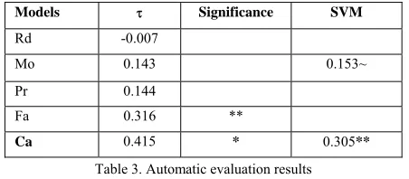
Table 3 gives automatic evaluation results. We can see that Mo and Pr got very close τ values (0.143 vs. 0.144). Meanwhile, Fa got better results (0.316), and the Ca achieved the best performance (0.415). The significance tests suggest that the difference between the τ values of Fa and Mo or Pr is significant, and so is the difference between the values of Ca and Fa, where *, **, ~ represent p-values <=0.01, (0.01, 0.05], and >0.05.
Table 3. Automatic evaluation results
Both Mo and Ca use the themes acquired by the classification. In comparison, we also used SVM to do the classification, and Table 3 lists the τ values for Mo and Ca. SVM is a typical supervised classification, which only uses the comparison between labeled data and unlabeled data. So, it generally requires a large number of training data to be effective. The results show that the difference between the performance of Mo with LP (0.143) and SVM (0.153) is not significant, while the difference between the performance of Ca with LP (0.415) and SVM (0.305) is significant.
On the contrary, for a negative τ value, the ordering can be considered to be worse than a random one. For a zero τ
value, the ordering is in fact close to a random one. So, percentage of τ values reflects quality of the orderings to some extent. Table 4 shows the percentage of positive ordering, negative orderings and median orderings for different models. It demonstrates that the cluster-adjacency based model produced the most positive orderings and the least negative orderings.
Models Positive Orderings
Negative Orderings
Median Orderings
Rd 99 (49.5%) 90 (45.0%) 11 (5.5%)
Mo 123 (61.5%) 64 (32.0%) 13 (6.5%)
Pr 125 (62.5%) 59 (29.5%) 16 (8.0%)
Fa 143 (71.5%) 38 (19.0%) 19 (9.5%)
Ca 162 (81.0%) 31 (15.5%) 7 (3.5%)
Table 4. Positive, Negative and Median Orderings
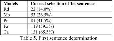
To see why the cluster-adjacency model achieved better performance, we checked about the determination of the first sentence between different models, since that it is extremely important for Pr, Fa and Ca, and it will influence later selections. Either in Pr or in Fa and Ca, it was assumed that there is one null sentence at the beginning of each source document. In Pr, to determine the first sentence is to find one which is the most likely to follow the assumed null sentence, while in the two adjacency models, to determine the first sentence means to select one which is the closest to the null sentence. Table 5 shows the comparison.
Models Correct selection of 1st sentences
Rd 22 (14.0%)
Mo 53 (26.5%)
Pr 81 (41.5%)
Fa 119 (59.5%)
Ca 131 (65.5%)
Table 5. First sentence determination
Table 5 indicates that cluster-adjacency model performed best in selection of the first sentence in the summaries. Another experiment we did is about how likely the k+1th sentence can be correctly selected if assuming that top k sentences have been successfully acquired. This is also useful to explain why a model performs better than others. Fig. 2 shows the comparison of the probabilities of correct determination of the k+1th sentence between different models. Fig. 2 demonstrates that the probabilities of the correct k+1th sentence selection in cluster-adjacency model are generally higher than those in other methods, which indicates that the cluster-adjacency model is more appropriate for the data.
0 0.2 0.4 0.6 0.8 1
1 2 3 4 5 6 7
Ca Fa MO Pr
Fig. 2. k+1th sentence determination
Table 6 gives the experiment results of the cluster-adjacency model with varying window ranges. In general, the cluster-adjacency model got better performance than feature-adjacency model without requirement of setting the noise elimination parameters. This can be seen as an advantage of Ca over Fa. However, we can see that the adjacency window size still influenced the performance as it did for Fa.
Window size τ values
2 0.314 3 0.415 4 0.398 5 0.356
Table 6. Ca performance with different window size
As a concrete example, consider a summary (D31050tG) in Fig. 3, which includes 6 sentences as the following.
0. After 2 years of wooing the West by signing international accords, apparently relaxing controls on free speech, and releasing and exiling three dissenters, China cracked down against political dissent in Dec 1998.
1. Leaders of the China Democracy Party (CDP) were arrested and three were sentenced to jail terms of 11 to 13 years.
2. The West, including the US, UK and Germany, reacted strongly. 3. Clinton's China policy of engagement was questioned.
4. China's Jiang Zemin stated economic reform is not a prelude to democracy and vowed to crush any challenges to the Communist Party or "social stability".
5. The CDP vowed to keep working, as more leaders awaited arrest.
Fig. 3. A sample summary
Table 7 gives the ordering generated by various models.
Models Output τ values
Pr 4 0 1 3 5 2 0.20
Mo 1 4 3 0 2 5 0.20
Fa 0 1 4 3 5 2 0.47
Ca 1 2 0 3 4 5 0.73
Table 7. Comparison: an example
tended to have higher feature-adjacency value. This is not contradicting with higher cluster-adjacency value between theme Null and theme 1. In fact, we found putting sentence 1 at the beginning was also acceptable subjectively.
In manual evaluation, the number of inversions was defined as the minimal number of interchanges of adjacent objects to transfer the output ordering to an acceptable ordering judged by human. We have three people participating in the evaluation, and the minimal, maximal and average numbers of interchanges for each summary among the three persons were selected for evaluation respectively. The Kendall’s τ of all 5 runs are listed in Table 8.
τ values
Models Average Minimal Maximal
Rd 0.106 0.202 0.034
Mo 0.453 0.543 0.345
Pr 0.465 0.524 0.336
Fa 0.597 0.654 0.423
Ca 0.665 0.723 0.457
Table 8. Manual evaluation results on 10 summaries
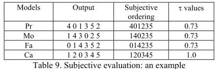
From table 7, we can find that all models get higher Kendall’s τ values than in automatic evaluation, and the two adjacency models achieved better results than Pr and Mo according to the three measures. As example, Table 9 lists the subjective evaluation for the sample summary in Fig. 3.
Models Output Subjective
ordering τ values
Pr 4 0 1 3 5 2 401235 0.73
Mo 1 4 3 0 2 5 140235 0.73
Fa 0 1 4 3 5 2 014235 0.73
Ca 1 2 0 3 4 5 120345 1.0
Table 9. Subjective evaluation: an example
6. Conclusion and Future Work
In this paper we propose a cluster-adjacency based model for sentence ordering in multi-document summarization. It learns adjacency information of sentences from the source documents and order sentences accordingly. Compared with the feature-adjacency model, the cluster-adjacency method produces sentence adjacency from cluster adjacency. The major advantage of this method is that it focuses on a kind of global adjacency (cluster on the whole), and avoids sensitivity to limited number of features, which in general is difficult. In addition, with semi-supervised classification, this method is expected to determine appropriate themes in source documents and achieve better performance.
Although the cluster-adjacency based ordering model solved the problem of noise elimination required by the feature-adjacency based ordering, how to set another parameter properly, i.e., the window range, is still unclear. We guess it may depend on length of source documents. The longer the source documents are, the bigger adjacency window size may be expected. But more experiments are needed to prove it.
In addition, the adjacency based model mainly uses only adjacency information to order sentences. Although it appears to perform better than models using only sequential
information on DUC2004 data set, if some sequential information could be learned definitely from the source documents, it should be better to combine the adjacency information and sequential information.
Reference
Regina Barzilay, Noemie Elhadad, and Kathleen R. McKeown. 2001. Sentence ordering in multidocument summarization. Proceedings of the First International Conference on Human Language Technology Research (HLT-01), San Diego, CA, 2001, pp. 149–156..
Barzilay, R N. Elhadad, and K. McKeown.2002. Inferring strategies for sentence ordering in multidocument news summarization. Journal of Artificial Intelligence Research, 17:35–55.
Sasha Blair-Goldensohn, David Evans. Columbia University at DUC 2004. In Proceedings of the 4th Document Understanding Conference (DUC 2004). May, 2004.
Danushka Bollegala, Naoaki Okazaki, Mitsuru Ishizuka. 2005. A machine learning approach to sentence ordering for multidocument summarization and it’s evaluation. IJCNLP 2005, LNAI 3651, pages 624-635, 2005. McKeown K., Barzilay R. Evans D., Hatzivassiloglou V., Kan M., Schiffman
B., &Teufel, S. (2001). Columbia multi-document summarization: Approach and evaluation. In Proceedings of DUC.
Mirella Lapata. Probabilistic text structuring: Experiments with sentence ordering. Proceedings of the annual meeting of ACL, 2003., pages 545– 552, 2003.
Nie Yu, Ji Donghong and Yang Lingpeng. An adjacency model for sentence ordering in multi-document Asian Information Retrieval Symposium (AIRS2006), Singapore., Oct. 2006.
Advaith Siddharthan, Ani Nenkova and Kathleen McKeown. Syntactic Simplication for Improving Content Selection in Multi-Document Summarization. In Proceeding of COLING 2004, Geneva, Switzerland. Tishby, N, Slonim, N. (2000) Data clustering by Markovian relaxation and
the Information Bottleneck Method. NIPS 13.
Szummer M. and T. Jaakkola. (2001) Partially labeled classification with markov random walks. NIPS14.
Zhu, X., Ghahramani, Z., & Lafferty, J. (2003) Semi-Supervised Learning Using Gaussian Fields and Harmonic Functions. ICML-2003.