Parameter Estimation for Statistical Parsing Models: Theory and Practice of

Parameter Estimation for Statistical Parsing Models:

Theory and Practice of Distribution-Free Methods

Michael Collins

AT&T Labs-Research.

[email protected]

Abstract

A fundamental problem in statistical parsing is the choice of criteria and algorithms used to estimate the parameters in a model. The predominant approach in computational linguistics has been to use a parametric model with some variant of maximum-likelihood estimation. The assumptions under which maximum-likelihood estimation is justified are arguably quite strong. As an alternative, we propose algorithms based on distribution-free analysis. We describe two algorithms based on these methods. The first uses boosting algorithms to rerank the output of an existing statistical parser. The second method uses the Perceptron or Support Vector Machine algorithms.

1

Introduction

A fundamental problem in statistical parsing is the choice of criteria and algorithms used to estimate the parameters in a model. The predominant approach in computational linguistics has been to use a parametric model with maximum-likelihood estimation, usually with some method for “smoothing” parameter estimates to deal with sparse data problems. Methods falling into this category include generative models such as Probabilistic Context-Free Grammars and Hidden Markov Models, Maximum Entropy models for tagging and parsing, and recent work on Markov Random Fields.

The first part of this paper discusses the statistical theory underlying various parameter-estimation methods. The assumptions under which maximum-likelihood estimation is justified are arguably quite strong – namely, that the structure of the process that generated the data is known (for example, maximum likelihood estimation for PCFGs is justified providing that the data was actually generated by a PCFG). In contrast, work in computational learning theory has concentrated on models with the weaker assumption that training and test examples are generated from the same distribution, but that the form of the distribution is unknown: in this sense the results hold across all distributions and are called "distribution-free". The result of this work – which goes back to results in statistical learning theory by Vapnik and colleagues, and to work within Valiant’s PAC model of learning – has been an explosion of algorithms and theory which provide radical alternatives to parametric maximum-likelihood methods. These algorithms are appealing in both theoretical terms, and in their impressive results in many experimental studies.

The second part of the paper discusses two parsing methods based on distribution-free training methods. The first uses boosting algorithms to rerank the output of an existing statistical parser. The second method uses the Perceptron or Support Vector Machine algorithms; a key insight is that these algorithms allow representation of parse trees through "kernels" – the paper discusses how the kernel trick can be used to give polynomial time algorithms for models with an exponential number of parameters, such as a representation tracking all subtrees of a tree (as in the DOP1 model for parsing [Bod 1998]).

2

Linear Models for Parsing

Say we have a context-free grammar (see [Hopcroft and Ullman 1979] for a formal definition)

G

=(

N;

Σ

;R;S

)

and possible string/tree pairs, in a language. We use

G

(

x

)for all

x

2 Σ

to denote the set of possible trees (parses) for the string

x

under the grammar (this set will be empty for strings not generated by the grammar).

A weighted grammar

G

=(

N;

Σ

;R;S;

Θ) also includes a parameter vectorΘwhich assigns a weight to each

rule in

R

. If there are

n

rules in

R

, thenΘ2<

n

(we assume that there is some arbitrary ordering

r

1

:::r

n

of

the rules in

R

, and that the

i

’th component ofΘis the weight on rule

r

i

).

Given a sentence

x

and a tree

y

spanning the sentence, we assume a function

(

x;y

)which tracks the counts

of the rules in(

x;y

). Specifically, the

i

’th component of

(

x;y

)is the number of times rule

r

i

is seen in(

x;y

).

Under these definitions, the weighted context-free grammar defines a function

h

from sentences to trees:

h

Θ(

x

)=arg max

y

2

G

(

x

)

(

x;y

)Θ (1)

Finding

h

Θ(

x

), the parse with the largest weight, can be achieved in polynomial time using a variant of the

CKY parsing algorithm (in spite of a possibly exponential number of members of

G

(

x

)).

In this paper we consider the structure of the grammar to be fixed, the learning problem being reduced to setting the values of the parametersΘ. The basic question is: given a “training sample” of sentence/tree pairs

f(

x

1

;y

1)

:::

(

x

m

;y

m

)g, what criterion should be used to set the weights in the grammar? A very common

method – that of Probabilistic Context-Free Grammars (PCFGs) – uses the parameters to define a distribution

P

(

x;y

jΘ)over possible sentence/tree pairs in the grammar. Maximum likelihood estimation is used to set

the weights. We will consider the assumptions under which this method is justified, and argue that these assumptions are quite strong. We will also give an example to show how PCFGs can be badly mislead when the assumptions are violated. As an alternative we will propose distribution-free methods for estimating the weights, which are justified under much weaker assumptions, and can give quite different estimates of the parameter values in some situations.

We would like to generalize weighted context-free grammars by allowing the representation

(

x;y

)to be

essentially any feature vector representation of the tree. There is still a grammar

G

, defining a set of candidates

G

(

x

)for each sentence. The parameters of the parser are a vectorΘ. The parser’s output is defined in the

same way as Eq. 1. The important thing in this generalization is that the representation

is now not necessarily directly tied to the productions in the grammar. This is essentially the approach advocated by [Johnson et al. 1999], although the criteria that we will propose for setting the parametersΘare quite different.

While superficially this might appear to be a minor change, it introduces two major challenges. The first is: how should the parameter values be set under these general representations? The PCFG method described in the next section, which results in simple relative frequency estimators of rule weights, is not applicable to more general representations. A generalization of PCFGs, Markov Random Fields (MRFs), has been proposed by several authors [Abney 1997; Johnson et al. 1999; Della Pietra et al. 1997]. This paper gives several alternatives to MRFs, and describes the theory and assumptions which underly various models.

A second challenge is that now that the parameters are not tied to rules in the grammar the CKY algorithm is not applicable – in the worst case we may have to enumerate all members of

G

(

x

)explicitly to find the

highest-scoring tree. One practical solution is to define the “grammar”

G

as a first pass statistical parser which allows dynamic programming to enumerate its top

n

candidates. A second pass uses the more complex representation

to choose the best of these parses. This is the approach used in [Collins 2000; Collins and Duffy 2001].

3

Probabilistic Context-Free Grammars

This section gives a review of the basic theory behind Probabilistic Context-Free Grammars (PCFGs). Say we have a context-free grammar

G

= (

N;

Σ

;R;S

) as defined in section 2. We will use T to denote the

set of all trees generated by

G

. Now say we assign a weight

p

(

r

)in the range 0 to 1 to each rule

r

in

R

.

Θ=flog

p

(

r

1)

;

log

p

(

r

2)

:::

log

p

(

r

n

)g. If

c

(

T;r

)is the number of times rule

r

is seen in a tree

T

, then the

“probability” of a tree

T

can be written as

P

(

T

jΘ)= Y

r

2

R

p

(

r

)

c

(

T;r

)

or equivalently log

P

(

T

jΘ)= X

r

c

(

T;r

)log

p

(

r

)=

(

T

)Θ

where we define

(

T

)to be an

n

-dimensional vector whose

i

’th component is

c

(

T;r

i

).

[Booth and Thompson 1973] give conditions on the weights which ensure that

P

(

T

jΘ)is a valid probability

distribution over the setT, in other words that P

T

2T

P

(

T

jΘ)=1, and8

T

2 T,

P

(

T

jΘ)0. The main

condition is that the parameters define conditional distributions over the alternative ways of rewriting each non-terminal symbol in the grammar. Formally, if we use

R

(

)to denote the set of rules whose left hand side

is some non-terminal

, then8

2

N;

P

r

2

R

(

)

p

(

r

)=1 and8

r

2

R

(

)

; p

(

r

)0. Thus the weight

associated with a rule

!

can be interpreted as a conditional probability

P

(

j

)of

rewriting as

(rather

than any of the other alternatives in

R

(

)).

1

We can now study how to train the grammar from a training sample of trees. Say there is a training set of trees

f

T

1

;T

2

:::T

m

g. Thelog-likelihoodof the training set given parametersΘis

L

(Θ)= P

j

log

P

(

T

j

jΘ). The

maximum-likelihood estimates are to take ˆΘ=arg maxΘ 2Ω

L

(Θ), whereΩis the set of allowable parameter

settings (i.e., the parameter settings which obey the constraints in [Booth and Thompson 1973]). It can be proved using constrained optimization techniques (i.e., using Lagrange multipliers) that the maximum-likelihood estimate for the weight of a rule

r

=

!

is

p

(

!

)=

P

j

c

(

T

j

;

!

)

=

P

j

c

(

T

j

;

)(here

we overload the notation

c

so that

c

(

)is the number of times non-terminal

is seen in

T

). So “learning” in

this case involves taking a simple ratio of frequencies to calculate the weights on rules in the grammar. So under what circumstances is maximum-likelihood estimation justified? Say there is a true set of weights

Θ

, which define an underlying distribution

P

(

T

jΘ

), and that the training set is a sample of size

m

from

this distribution. Then it can be shown that as

m

increases to infinity, then with probability 1 the parameter estimates ˆΘconverge to the “true” parameter valuesΘ

.

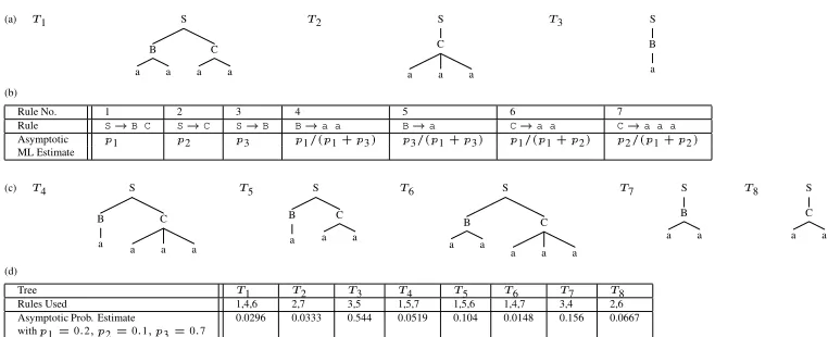
To illustrate the deficiencies of PCFGs, we give a simple example. Say we have a random process which generates just 3 trees, with probabilitiesf

p

1

;p

2

;p

3g, as shown in figure 1(a). The training sample will consist

of a set of trees drawn from this distribution. A test sample will be generated from the same distribution, but in this case the trees will be hidden, and only the surface strings will be seen (i.e.,h

aaaa

i,h

aaa

iandh

a

iwith

probabilities

p

1

;p

2

;p

3respectively). We would like to learn a weighted CFG with as small error as possible on

a randomly drawn test sample.

As the size of the training sample goes to infinity, the relative frequencies of treesf

T

1

;T

2

;T

3gin the training

sample will converge tof

p

1

;p

2

;p

3g. This makes it easy to calculate the rule weights that maximum-likelihood

estimation converges to – see figure 1(b). We will call the PCFG with these asymptotic weights theasymptotic PCFG. Notice that the grammar generates trees never seen in training data, shown in figure 1(c). The grammar is ambiguous for stringsh

aaaa

i(both

T

1and

T

4are possible) andh

aaa

i(

T

2and

T

5are possible). In fact, under

certain conditions

T

4and

T

5will get higher probabilities under the asymptotic PCFG than

T

1and

T

2, and both

stringsh

aaaa

iandh

aaa

iwill be misparsed. Figure 1(d) shows the distribution of the asymptotic PCFG over

the 8 trees when

p

1 =0

:

2

;p

2 =0

:

1 and

p

3 =0

:

7. In this case both ambiguous strings are misparsed by the

asymptotic PCFG, resulting in an expected error rate of(

p

1+

p

2)=30% on newly drawn test examples.

This is a striking failure of the PCFG when we consider that it is easy to derive weights on the grammar rules which parse both training and test examples with no errors.2 _{On this example there exist weighted grammars}

which make no errors, but the maximum likelihood estimation method will fail to find these weights, even with unlimited amounts of training data.

1_{[Booth and Thompson 1973] also give a second, technical condition on the probabilities}

p(r), which ensures that the probability of a

derivation halting in a finite number of steps is 1.

2_{Given any finite weights on the rules other thanB}

! a, it is possible to set the weightB ! asufficiently low forT1andT2to get

(a) T Asymptotic Prob. Estimate 0.0296 0.0333 0.544 0.0519 0.104 0.0148 0.156 0.0667 withp

1=0:2;p

2=0:1;p

3=0:7

Figure 1: (a) Training and test data consists of trees

T

1,

T

2 and

T

3 drawn with probabilities

p

1

;p

2 and

p

3.

(b) The ML estimates of rule probabilities converge to simple functions of

p

1

;p

2

;p

3as the training size goes

to infinity. (c) The grammar also generates

T

4

:::T

8, which are never seen in training or test data. (d) The

probabilities assigned to the trees as the training size goes to infinity, for

p

1=0

:

2

;p

2=0

:

1

;p

3=0

:

7.

4

Theory

This section introduces a general framework for supervised learning problems. There are several books [Devroye et. al 1996; Vapnik 1998; Cristianini and Shawe-Taylor 2000] which cover the material in detail. We will use this framework to analyze both parametric methods (PCFGs, for example), and the distribution–free methods proposed in this paper. We assume the following:

An input domainX and an output domainY. The task will be to learn a function mappingX toY. In

parsing,X is a set of possible sentences andYis a set of possible trees.

There is some underlying probability distribution

D

(

x;y

)overXY. The distribution is used to generate

both training and test examples. It is an unknown distribution, but it is constant across training and test examples.

There is a loss function

L

(

y;

y

ˆ)which measures the cost of proposing an output ˆ

y

when the “true” output is

y

.

A commonly used cost is the 0-1 loss

L

(

y;

y

ˆ)=0 if

y

=

y

ˆ, and

L

(

y;

y

ˆ)=1 otherwise. We will concentrate

on this loss function in this paper.

Given a function

h

fromX toY, itsexpected lossis

Er

(

h

)= P

x;y

D

(

x;y

)

L

(

y;h

(

x

)). Under 0-1 loss this

is the expected proportion of errors that the hypothesis makes on examples drawn from the distribution

D

. We would like to learn a function whose expected loss is as low as possible –

Er

(

h

)is a measure of how

successful a function

h

is. Unfortunately, because we do not have direct access to the distribution

D

, we cannot explicitly calculate the expected loss of a hypothesis.

The training set is a sample of

m

pairs f(

x

1

;y

1)

;:::;

(

x

m

;y

m

)g drawn from the distribution

D

. This

is the only information we have about

D

. Theempirical loss of a function

h

on the training sample is ˆ

Er

(

h

)=

1

m

P

i

L

(

y

i

;h

(

x

i

)).

A useful concept is theBayes Optimalhypothesis, which we will denote as

h

B

. It is defined as

h

B

(

x

)=

arg max

y

2Y

D

(

x;y

). The Bayes optimal hypothesis simply outputs the most likely

y

under the distribution

D

for each input

x

. It is easy to prove that this function minimizes the expected loss

Er

(

h

)over the space of all

possible functions – the Bayes optimal hypothesis cannot be improved upon. Unfortunately, in general we do not know

D

(

x;y

), so the Bayes optimal hypothesis, while useful as a theoretical construct, cannot be obtained

directly in practice. Given that the only access to the distribution

D

(

x;y

)is indirect, through a training sample

4.1

Parametric Models

Parametric models attempt to solve the supervised learning problem by explicitly modeling either the joint distribution

D

(

x;y

)or the conditional distributions

D

(

y

j

x

)for all x.

In the joint distribution case, there is a parameterized probability distribution

P

(

x;y

jΘ). As the parameter

valuesΘare varied the distribution will also vary. The parameter spaceΩis a set of possible parameter values for which

P

(

x;y

jΘ)is a well-defined distribution (i.e., for which

P

x;y

P

(

x;y

jΘ)=1).

A crucial assumption in parametric approaches is that there is someΘ

2Ωsuch that

D

(

x;y

)=

P

(

x;y

jΘ

).

In other words, we assume that

D

is a member of the set of distributions under consideration. Now say we have a training samplef(

x

1

;y

1)

:::

(

x

m

;y

m

)gdrawn from

D

(

x;y

). A common estimation method is to set

the parameters to the maximum-likelihood estimates, ˆΘ=arg max P

i

log

P

(

x

i

;y

i

jΘ). Under the assumption

that

D

(

x;y

)=

P

(

x;y

jΘ

)for someΘ

2Ω, for a wide class of distributions it can be shown that

P

(

x;y

jΘˆ)

converges to

D

(

x;y

)in the limit as the training size

m

goes to infinity. Because of this, if we consider the

function ˆ

h

(

x

) = arg max

y

2Y

P

(

x;y

jΘˆ), then in the limit ˆ

h

(

x

)will converge to the Bayes optimal function

h

B

(

x

). So under the assumption that

D

(

x;y

)=

P

(

x;y

jΘ

)for someΘ

2Ω, and with infinite amounts of

training data, the maximum-likelihood method is provably optimal.

Methods which model the conditional distribution

D

(

y

j

x

) are similar. The parameters now define a

conditional distribution

P

(

y

j

x;

Θ). The assumption is that there is some Θ

such that 8

x; D

(

y

j

x

) =

P

(

y

j

x;

Θ

). Maximum-likelihood estimates can be defined in a similar way, and in this case the function

ˆ

h

(

x

)=arg max

y

2Y

P

(

y

j

x;

Θˆ)will converge to the Bayes optimal function

h

B

(

x

)as the sample size goes to

infinity.

4.2

An Overview of Distribution-Free Methods

From the arguments in the previous section, parametric methods are optimalproviding that the distribution generating the data is in the class of distributions being considered. But what happens if this assumption is violated? In this case there are no guarantees on the expected error rate of the maximum-likelihood method. The example in section 3 shows how maximum-likelihood estimation can be badly mislead when the distribution generating the data is not in the class being considered.

This paper proposes alternatives to maximum-likelihood methods which give theoretical guarantees without making the assumption that the distribution generating the data comes from some predefined class. The only assumption is that the same distribution generates both training and test examples. These methods also provide bounds on how many training samples are required for learning, dealing with the case where there is only a finite amount of training data. Thus the methods address a second weakness of the parametric approach:the guarantees of ML estimation are asymptotic, holding only in the limit as the training data size goes to infinity.

A crucial idea in distribution-free learning is that of ahypothesis space. This is a set of functions under consideration, each member of the set being a function

h

: X ! Y. For example, in weighted context-free

grammars the hypothesis space isH= f

h

Θ(

x

)= arg max

y

2

G

(

x

)

(

x;y

)Θ: Θ 2 <

n

g. So each possible

parameter setting defines a different function from sentences to trees, andHis the infinite set of all such

functions asΘranges over the parameter space<

n

.

Learning is then usually framed as the task of choosing a “good” function inHon the basis of a training

sam-ple as evidence. Recall the definition of the expected error of a hypothesis

Er

(

h

)= P

x;y

D

(

x;y

)

L

(

y;h

(

x

)).

We will use

h

to denote the “best” function in H by this measure,

h

= arg min

h

2H

Er

(

h

) =

arg min

h

2H P

x;y

D

(

x;y

)

L

(

y;h

(

x

)). A first learning method to study is as follows. Given a training sample (

x

i

;y

i

)for

i

= 1

:::m

, the method simply chooses the hypothesis with minimum empirical error, that is

ˆ

h

=arg min

h

2H

ˆ

Er

(

h

)=arg min

h

2H

1

m

P

i

L

(

y

i

;h

(

x

i

)). This strategy is called “Empirical Risk

Minimiza-tion” by Vapnik [Vapnik 1998]. Two questions which arise are:

of the best function in the set,

Er

(

h

), regardless of the underlying distribution

D

(

x;y

)? In other words, is

this method of choosing a hypothesis always consistent?

The answer to this depends on the nature of the hypothesis spaceH. For finite hypothesis spaces the ERM

method is always consistent. For many infinite hypothesis spaces, such as the weighted grammar example above, the method is also consistent. However, some infinite hypothesis spaces can lead to the method being inconsistent – specifically, if a measure called the VC dimension [Vapnik 1998] ofHis infinite, the ERM

method may be inconsistent. Intuitively, the VC dimension can be thought of as a measure of the complexity of an infinite set of hypotheses.

If the method is consistent, how quickly does

Er

(

h

ˆ)converge to

Er

(

h

)? In other words, how much training

data is needed to have a good chance of getting close to the best function inH? We will see in the next

section that the convergence rate depends on various measures of the “size” of the hypothesis space. For finite sets, the rate of convergence depends directly upon the size ofH. For infinite sets, several measures

have been proposed – we will concentrate on rates of convergence based on a concept called themarginof a hypothesis on training examples.

4.3

Convergence Results for Hyperplane Classifiers

This section describes analysis applied for binary classifiers, where the set Y = f 1

;

+1g. We consider

hyperplane classifiers, where a linear separator in some feature space is used to separate examples into the two classes. Hyperplane classifiers go back to one of the earliest learning algorithms, the Perceptron algorithm [Rosenblatt 1958]. There has been a large amount of effort devoted to the theory of hyperplane classifiers. They are similar to the linear models for parsing we proposed in section 2 (in fact the framework of section 2 can be viewed as a generalization of hyperplane classifiers). We will initially review some results applying to linear classifiers, and then discuss how various results may be applied to parsing.

We will discuss a hypothesis space of

n

-dimensional hyperplane classifiers, defined as follows:

Each instance

x

is represented as a vector

(

x

)in<

n

.

For given parameter valuesΘ 2<

n

and a bias parameter

b

2 <, the output of the classifier is

h

Θ

;b

(

x

)=

sign

(

x

)Θ+

b

where sign(

z

)is+1 if

z

0, 1 otherwise. There is a clear geometric interpretation

of this classifier. The points

(

x

) are in

n

-dimensional Euclidean space. The parametersΘ

;b

define a

hyperplane through the space, the hyperplane being the set of points

z

such that(

z

Θ+

b

)=0. This is a

hyperplane with normalΘ, at distance

b=

jjΘjjfrom the origin. This hyperplane is used to classify points: all

points falling on one side of the hyperplane are classified as+1, points on the other side are classified as 1.

The hypothesis space is the set of all hyperplanes,H=f

h

Θ

;b

(

x

):Θ2<

n

;b

2<g.

It can be shown that the ERM method is consistent for hyperplanes, through a method called VC analysis [Vapnik 1998]. We will not go into details here, but roughly speaking, the VC-dimension of a hypothesis space is a measure of its size or complexity. A set of hyperplanes in<

n

has VC dimension of(

n

+1). For any

hypothesis space with finite VC dimension the ERM method is consistent.

An alternative to VC-analysis is to analyse hyperplanes through properties of “margins” on training examples. First consider the case where a training samplef(

x

1

;y

1)

:::

(

x

m

;y

m

)g is “linearly separable” – there is a

hyperplane which achieves 0 errors on the training data. Then for each hyperplane with 0 error (there will in general be more than one), themarginon the training set for hyperplane

h

Θ

;b

is defined as3

Θ

;b

=min

i

y

i

(

x

i

)Θ+

b

jjΘjj

(2)

3

jjΘjjis the Euclidean norm, q

P

j

Θ2

The margin

Θ

;b

has a simple geometric interpretation: it is the minimum distance of any training point to the hyperplane defined byΘ

;b

. The following theorem then holds:

Theorem 1 Special case of [Cristianini and Shawe-Taylor 2000] Theorem 4.19. Assume the hypothesis class

His a set of hyperplanes, and that there is some distribution

D

(

x;y

)generating examples. Let

R

be a constant

such that8

x;

jj

(

x

) jj

R

. For all

h

Θ

;b

2Hwith zero error on the training sample, with probability at least

The bound is minimized for the hyperplane with maximum margin (i.e., maximum value for

Θ

;b

) on the training sample. This bound suggests that if the training data is separable, the hyperplane with maximum margin should be chosen as the hypothesis with the best bound on its expected error. It can be shown that the maximum margin hyperplane is unique, and can be found efficiently using algorithms described in section 5.2. Search for the maximum-margin hyperplane is the basis of “Support Vector Machines” (hard-margin version) [Vapnik 1998]. The previous theorem does not apply when the training data cannot be classified with 0 errors by a hyperplane. There is, however, a similar theorem that can be applied in the non-separable case. First, define ˆ

L

(

h

Θ

;b

;

)to

be the proportion of examples on training data with margin less than

for the hyperplane

h

Θ

;b

:

ˆ

The following theorem can now be stated:

Theorem 2 [Cristianini and Shawe-Taylor 2000] Theorem 4.19. Assume the hypothesis classHis a set of

hyperplanes, and that there is some distribution

D

(

x;y

)generating examples. Let

R

be a constant such that

8

x;

jj

(

x

) jj

R

. For all

h

Θ

;b

2H, for all

>

0, with probability at least1

over the choice of training set

This result is important in cases where a large proportion of training samples can be classified with relatively large margin, but a relatively small number of outliers make the problem inseparable, or force a small margin. The result suggests that in some cases a few examples are worth “giving up on”, resulting in the first term in the bound being larger than 0, but the second term being much smaller due to a larger value for

. Thesoft margin

version of Support Vector Machines [Cortes and Vapnik 1995], described in section 5.2, attempts to explicitly manage the trade-off between the two terms in the bound.

A similar bound, due to [Schapire et al. 1998], involves a margin definition which depends on the 1-norm rather than the 2-norm of the parametersΘ(jjΘjj1is the 1-norm,

P

Theorem 3 [Schapire et al. 1998] Assume the hypothesis classHis a set of hyperplanes in<

n

, and that there

is some distribution

D

(

x;y

)generating examples. For all

h

Θ

;b

2H, for all

>

0, with probability at least

Input:Examplesf(

x

1

;y

1)

:::

(

x

m

;y

m

)g, Grammar

G

, representation

:XY!<

n

Algorithm: Initialise parametersΘto be 0 For

t

= 1 to

T

, For

i

= 1 to

m

,

Figure 2: The perceptron algorithm for parsing. It takes

T

passes over the training set.

4.4

Application of Margin Analysis to Parsing

We now consider how the theory for hyperplane classifiers might apply to the linear models for parsing described in section 2. The method for converting parsing to a margin-based problem is very similar to the method for ranking problems described in [Freund et al. 1998]. As a first step, we can define the concept of margin on the training set, which is analogous to the definition in Eq. 2 of the margin for hyperplane classifiers:

Θ= min

The margin on the training set is now the minimum difference between the correct tree for a sentence and the next highest scoring tree for that sentence. The first SVM algorithm described in section 5.2 searches for the parameter values which give the maximum value for

Θ.

The bounds in theorems 2 and 3 suggested a tradeoff between keeping the values for ˆ

L

(

h

Θ

;b

;

)and ˆ

L

1(

h

Θ

;b

;

)

low and keeping the value of

high. For parsing, we suggest the following analogous terms to ˆ

L

and ˆ

L

1:

ˆ

The algorithms described in section 5 attempt to find a hypothesisΘwhich can achieve low values for these quantities with a high value for

. The algorithms are direct modifications of algorithms for learning hyperplane classifiers for binary classification. The bounds in theorems 2 and 3 do not apply to the parsing case, but it is likely that similar theorems apply – we leave this to future work. Theorem 6 of [Schapire et al. 1998] treats a similar case to the parsing example, and it is likely that this this proof holds for the parsing set-up.

5

Algorithms

5.1

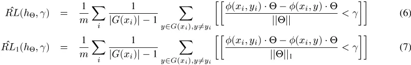
A Variant of the Perceptron Algorithm for Parsing

The first algorithm for setting the parameter valuesΘis the perceptron algorithm, as introduced by [Rosenblatt 1958]. Figure 2 shows the algorithm. Note that the main computational difficulty is in calculating

y

=

h

Θ(

x

i

)

for each example in turn. For weighted context-free grammars this step can be achieved in polynomial time using the CKY parsing algorithm. Thus for the weighted CFG representation, the perceptron algorithm is relatively efficient. Other representations may have to rely on explicitly calculating

(

x

i

;z

)Θfor all

z

2

G

(

x

i

), and

hence depend computationally on the number of candidatesj

G

(

x

i

)jfor

i

=1

:::m

.

It is useful to define the maximum-achievable margin

on a separable training set as

=maxΘ 2<

. The following theorem can then be stated:

Theorem 4 (Simple modification of theorem from [Block 1962; Novikoff 1962], see also [Freund and Schapire 1999]). Let f(

x

1

;y

1)

:::

(

x

n

;y

n

)g be a sequence of examples such that 8

i;

8

y

2

G

(

x

i

)

;

jj

(

x

i

;y

i

)

(

x

i

;y

)jj

R

. Assume the sequence is separable, and take

to be the maximum

achievable margin on the sequence. Then the number of mistakes made by the perceptron algorithm on this sequence is at most(

R=

)

2_.

This theorem implies that if the training sample in figure 2 is separable, and we iterate the algorithm repeatedly over the training sample (i.e.,

T

!1), then the algorithm converges to a parameter setting that classifies the

training set with zero errors. Thus we now have an algorithm for training weighted context-free grammars which will find a zero error hypothesis if it exists. For example, the algorithm would find a weighted grammar with zero expected error on the example problem in section 3.

5.2

Support Vector Machines

Now consider search for the maximum margin hyperplane, the hypothesisΘwith maximum value for

Θ(Eq. 5). It can be shown [Vapnik 1998] that the parameter values which give the maximum-margin solution can be found by minimizingjjΘjj

2_{subject to the constraints}

8

i;

8

y

2

G

(

x

i

)s.t.

y

6=

y

i

;

(

x

i

;y

i

)Θ

(

x

i

;y

)Θ1.

Thus there are

P

i

(j

G

(

x

i

)j 1)= P

i

j

G

(

x

i

)j

m

constraints.

Next, consider search for a hypothesisΘwhich has a low value of ˆ

RL

(

h

Θ

;

)(Eq. 6) for some relatively

large value of

. [Cortes and Vapnik 1995] suggest the following constrained optimization problem: minimize

jjΘjj

2

+

C

P

i;y

2

G

(

x

i)

;y

6=

y

i

(

i;y

)subject to the constraints8

i;

8

y

2

G

(

x

i

)s.t.

y

6=

y

i

;

(

x

i

;y

i

)Θ

(

x

i

;y

)Θ1

(

i;y

). Here

(

i;y

)are a set of “slack variables”. Any examples(

i;y

)with

(

i;y

)=0 are

classified with at least a margin of 1

=

jjΘjj; any examples with a positive–valued slack variable are classified

with a margin less than 1

=

jjΘjj. The variable

C

is a constant which manages the balance between keeping

jjΘjj

2

small and the slack variables small. As

C

!1, the problem becomes the same as the hard-margin SVM

problem, and the method attempts to find a hyperplane which correctly separates all examples with margin at least 1

=

jjΘjj(i.e., all slack variables are 0). For smaller

C

, the training algorithm may “give up” on some

examples (i.e., set

(

i;y

)

>

0) in order to keepjjΘjj

2_{low. Thus by varying}

C

_{, the method effectively modifies}

the trade-off between the two terms in the bound in Theorem 2. In practice, a common approach is to train the model for several values of

C

, and then to pick the classifier which has best performance on some held-out set of development data.

Both kinds of SVM optimization problem have been studied extensively (e.g., see [Joachims 1998; Platt 1998]) and can be solved relatively efficiently. (A publicly available package for Support Vector Machines, written by Thorsten Joachims, is available fromhttp://ais.gmd.de/˜ thorsten/svm light/.)

5.3

Boosting

The AdaBoost algorithm [Freund and Schapire 1997] is one method for optimizing the bound in The-orem 3 [Schapire et al. 1998]. Figure 3 shows the AdaBoost algorithm, altered slightly so that it applies to the parsing problem. The algorithm converts the training set into a set of triples: T =

f(

x

i

;y

i

;y

):

i

=1

:::m;y

2

G

(

x

i

)s.t.

y

6=

y

i

g. Each member (

x;y

1

;y

2) of T is a triple such that

x

is

a sentence,

y

1 is the correct tree for that sentence, and

y

2 is an incorrect tree also proposed by

G

(

x

).

AdaBoost maintains a distribution

D

t

over the training examples such that

D

t

(

x;y

1

;y

2)is proportional to

expf Θ

(

x;y

1)

(

x;y

2)

g. Members ofT which are well discriminated by the current parameter values

Θare given low weight by the distribution, whereas examples which are poorly discriminated are weighted more highly. The

s

’th component ofΘhas

r

s

as a measure of how well correlated it is with the current distribution,

r

s

= P

(

x;y

1

;y

2)2T

D

t

(

x;y

1

;y

2)

s

(

x;y

1)

s

(

x;y

2)

. The magnitude of

r

s

can be taken as a measure of how correlated

s

(

x;y

1)

s

(

x;y

2)

is with the distribution

D

t

. If it is highly correlated,j

r

s

jwill be large,

and the

s

’th parameter will be useful in driving down the margins on the more highly weighted members ofT.

In fact, there is a strong relation between the values ofj

r

s

j, and the margin-based bound in Theorem 3. If we

define

t

=(1 j

r

s

t

j)

=

2 then the following theorem holds:

Theorem 5 (Slight Modification of Theorem 5 of [Schapire et al. 1998]). If we define

RL

ˆ 1(

h

Θ

;

)as in Eq. 7,

and the Adaboost algorithm in figure 3 generates values

1

;

2

;:::

T

, then for all

,

ˆ

RL

1(

h

Θ

;

)2

T

T

Y

t

=1 q

1

t

(1

t

)

Input: Examplesf(

x

1

;y

1)

:::

(

x

m

;y

m

)g, Grammar

G

, representation

:X Y !<

n

such that8(

x;y

1

;y

2) 2 T

;

Set initial parameter valuesΘ=0

For

t

=1 to

T

– Define a distribution over the training sampleT as

8(

x;y

1

;y

2)2T

; D

– Update single parameterΘ

s

t =Θ

s

Figure 3: The AdaBoost algorithm applied to parsing.

[Schapire et al. 1998] point out that if for all

t

=1

:::T

,

t

1

=

2

(i.e.,j

r

s

decreases exponentially in the number of iterations,

T

. So if the AdaBoost algorithm can successfully maintain high values ofj

r

s

t

jfor several iterations, it will be successful at minimizing ˆ

RL

1(

h

Θ

;

)for a relatively large

range of

, and by implication it will be successful in optimizing the bound in Theorem 3. In practice, a set of held-out data is usually used to optimize

T

, the number of rounds of boosting.

The algorithm states a restriction on the representation

. For all members(

x;y

1

;y

2)ofT, for

s

=1

:::n

,

s

(

x;y

1)

s

(

x;y

2)

must be in the range 1 to+1. This is not as restrictive as it might seem. If

is always

strictly positive, it can be rescaled so that its components are always between 0 and+1. If some components

may be negative, it suffices to rescale the components so that they are always between 0

:

5 and+0

:

5. A

common use of the algorithm, as applied in [Collins 2000], is to have the

n

components of

to be the values of

n

indicator functions, in which case all values of

are either 0 or 1, and the condition is satisfied.

5.4

Dual forms of the Perceptron and SVM Algorithms

In the boosting algorithms, the training set was effectively converted into a set of triples,T (see figure 3). This

set is of size

M

=

Now consider an alternative form for the perceptron algorithm, shown in figure 4. The algorithm does not explicitly represent the parameter vectorΘ, but instead maintains weights

j

over the

M

examples in the training set. These “dual” variables

j

do, however, implicitly define the parameter vectorΘ, through the identityΘ=

. For example, the ranking score for a new example(

x;y

)can

Input:Examplesf(

x

1

;y

1)

:::

(

x

m

;y

m

)g, Grammar

G

, representation

:XY!<

n

Algorithm:

Initialise

j

=0 for

j

=1

:::M

For

t

= 1 to

T

, For

i

= 1 to

m

,

Calculate

y

=arg max

z

2

G

(

x

i )

P

j

=1

:::M

j

(

x

0

j

;y

0

j

)

(

x

i

;z

)

(

x

0

j

;z

0

j

)

(

x

i

;z

)

If(

y

=

y

i

)then do nothing; else if(

y

6=

y

i

)then

I

(

i;y

)

=

I

(

i;y

)

+1

Output:The dual parameters

j

. Output on a new sentence

x

is arg max

y

2

G

(

x

)

P

j

j

(

x

0

j

;y

0

j

)

(

x;y

)

(

x

0

j

;z

0

j

)

(

x;y

)

Figure 4: The perceptron algorithm for parsing in dual form.

It can be verified that the algorithm in 4 is completely equivalent to the perceptron algorithm in 2: we will refer to the algorithm in 4 as the perceptron algorithm in “dual form”.

The dual form is useful because for some representations the dual form algorithm is much more computation-ally efficient than the usual algorithm. This occurs when the inner product between two examples(

x

1

;y

2)and

(

x

2

;y

2)(i.e.,

(

x

1

;y

1)

(

x

2

;y

2)) can be computed efficiently, in spite of the representation

being very high

dimensional. See chapter 3 of [Cristianini and Shawe-Taylor 2000] for examples of many such representations. To illustrate this, we will consider one particular representation as an example. The DOP1 model [Bod 1998] describes a representation which keeps track of all subtrees seen in training data. We will consider linear models with this representation:

(

x;y

)has as many components as there are subtrees in training data, and it

tracks the count of each of these subtrees in the example(

x;y

). This is a very high dimensional representation,

because in general a tree has an exponential number of subtrees. This makes the perceptron algorithm in its original form (figure 2) prohibitively inefficient – directly computingΘ

(

x;y

)for some example will take

time linear in the number of subtrees of

(

x;y

), an exponential number.

In contrast, it turns out that the dual form algorithm can be applied to the problem efficiently. The key to this is that the inner product between any two trees,

(

x

1

;y

1)

(

x

2

;y

2), can be calculated in polynomial time

using dynamic programming, in spite of the size of

. See [Collins and Duffy 2001] for details. Armed with a subroutine which calculates

(

x

1

;y

1)

(

x

2

;y

2)for any two trees efficiently, the dual form algorithm can find

a set of dual parameters which define a separating hyperplane in the DOP1 representation space.

The SVM algorithms have a similar dual form: the final hypothesis (maximum margin hyperplane) can be expressed through a linear combination of training examples (as in Eq. 8), and the optimization problem can be solved through calculations involving inner products between training examples.

6

Conclusions

This paper has described a number of methods for learning statistical grammars. All of these methods have several components in common: the choice of a grammar which defines the set of candidates for a given sentence, and the choice of representation of parse trees. A score indicating the plausibility of competing parse trees is taken to be a linear model, the result of the inner product between a tree’s feature vector and the vector of model parameters. The only respect in which the methods differ is in how the parameter values (the “weights” on different features) are calculated using a training sample as evidence.

drawn test examples. The goal of learning is to use the training data as evidence for choosing a function which has small expected loss.

A central idea in the analysis of learning algorithms is that of the margins on examples in training data. We described theoretical bounds which motivate approaches which attempt classify a large proportion of examples in training with a large margin. Finally, we described several algorithms which can be used to achieve this goal on the parsing problem.

Acknowledgements.I would like to thank Sanjoy Dasgupta, Yoav Freund, John Langford, David McAllester, Rob Schapire and Yoram Singer for answering many of the questions I have had about the learning theory and algorithms in this paper. Thanks also to Nigel Duffy, for many useful discussions while we were collaborating on the use of kernels for parsing problems.

References

[Abney 1997] Abney, S. (1997). Stochastic attribute-value grammars.Computational Linguistics, 23, 597-618.

[Block 1962] Block, H. D. 1962. The perceptron: A model for brain functioning.Reviews of Modern Physics, 34, 123–135. [Bod 1998] Bod, R. 1998.Beyond Grammar: An Experience-Based Theory of Language. CSLI Publications/Cambridge

University Press.

[Booth and Thompson 1973] Booth, T. L., and Thompson, R. A. 1973. Applying Probability Measures to Abstract Lan-guages.IEEE Transactions on Computers, C-22(5), 442–450.

[Collins 2000] Collins, M. (2000). Discriminative Reranking for Natural Language Parsing. InProceedings of the Seven-teenth International Conference on Machine Learning (ICML 2000). San Francisco: Morgan Kaufmann.

[Collins and Duffy 2001] Collins, M. and Duffy, N. 2001. Parsing with a Single Neuron: Convolution Kernels for Natural Language Problems. Technical Report, University of California at Santa Cruz.

[Cortes and Vapnik 1995] Cortes, C. and Vapnik, V. 1995. Support–Vector Networks. InMachine Learning, 20(3):273-297. [Cristianini and Shawe-Taylor 2000] Cristianini, N. and Shawe-Taylor, J. 2000.An introduction to support vector machines

(and other kernel-based learning methods). Cambridge University Press.

[Della Pietra et al. 1997] Della Pietra, S., Della Pietra, V., & Lafferty, J. (1997). Inducing features of random fields.IEEE Transactions on Pattern Analysis and Machine Intelligence, 19, 380–1.593.

[Devroye et. al 1996] Devroye, L., Gyorfi, L., and Lugosi, G. 1996.A Probabilistic Theory of Pattern Recognition. Springer. [Freund and Schapire 1997] Freund, Y. and Schapire, R. (1997). A decision-theoretic generalization of on-line learning

and an application to boosting.Journal of Computer and System Sciences, 55(1):119–139, August 1997.

[Freund and Schapire 1999] Freund, Y. and Schapire, R. (1999). Large Margin Classification using the Perceptron Algo-rithm. InMachine Learning, 37(3):277–296.

[Freund et al. 1998] Freund, Y., Iyer, R.,Schapire, R.E., & Singer, Y. 1998. An efficient boosting algorithm for combining preferences. InMachine Learning: Proceedings of the Fifteenth International Conference. Morgan Kaufmann. [Hopcroft and Ullman 1979] Hopcroft, J. E., and Ullman, J. D. 1979.Introduction to automata theory, languages, and

computation. Reading, Mass.: Addison–Wesley.

[Joachims 1998] Joachims, T. 1998. Making large-Scale SVM Learning Practical. In [Scholkopf et al. 1998].

[Johnson et al. 1999] Johnson, M., Geman, S., Canon, S., Chi, S., & Riezler, S. (1999). Estimators for stochastic ‘unification-based” grammars. InProceedings of the 37th Annual Meeting of the Association for Computational Lin-guistics. San Francisco: Morgan Kaufmann.

[Novikoff 1962] Novikoff, A. B. J. 1962. On convergence proofs on perceptrons. InProceedings of the Symposium on the Mathematical Theory of Automata, Vol XII, 615–622.

[Platt 1998] Platt, J. 1998. Fast Training of Support Vector Machines using Sequential Minimal Optimization. In [Scholkopf et al. 1998].

[Rosenblatt 1958] Rosenblatt, F. 1958. The Perceptron: A Probabilistic Model for Information Storage and Organization in the Brain.Psychological Review, 65, 386–408. (Reprinted inNeurocomputing(MIT Press, 1998).)

[Schapire et al. 1998] Schapire R., Freund Y., Bartlett P. and Lee W. S. 1998. Boosting the margin: A new explanation for the effectiveness of voting methods.The Annals of Statistics, 26(5):1651-1686.

[Scholkopf et al. 1998] Scholkopf, B., Burges, C., and Smola, A. (eds.). (1998).Advances in Kernel Methods – Support Vector Learning, MIT Press.