Mathematical Results on Quantum Many body Physics

(1)

Mathematical results on quantum many-body physics

Thesis by

Marius Lemm

In Partial Fulllment of the Requirements for the degree of

Doctor of Philosophy

CALIFORNIA INSTITUTE OF TECHNOLOGY Pasadena, California

2017

(2)

c

2017

Marius Lemm

ORCID: 0000-0001-6459-8046

(3)

ACKNOWLEDGEMENTS

First and foremost, I want to thank Rupert L. Frank for being a wonderful ad-visor. Of course, I am grateful for the diverse and interesting mathematics that he shared with me over the years, for his advice on the small and large matters that may concern a Ph.D. student, and for his unwavering commitment not to wave hands, but rather to explain critical details with admirable precision. Most of all, though, I am grateful that he always struck a well-measured bal-ance between being engaged and interested in my progress, while giving me the freedom to develop and pursue my personal tastes. Danke, Rupert! The Caltech math department, small in size, has been a warm and welcoming place since the day I arrived. I especially want to thank Professors Nets Katz, Vlad Markovic and Barry Simon for advice and for the pleasure of collabora-tion, and Peter Burton for being an amicable and always-patient oce mate. On many mornings, the sta at the math oce, previously Kathy Carreon, Stacey Croomes and Kristy Thompson, and more recently Elsa Echegaray, Meagan Heirwegh and Michelle Vine, have made my day a little brighter and I thank them for that.

(4)

ABSTRACT

The collective behavior exhibited by a large number of microscopic quantum particles is at the heart of some of the most striking phenomena in condensed-matter physics such as Bose-Einstein condensation and superconductivity. Physicists and mathematicians have made great progress in understanding when and how these collective phenomena emerge through the interplay of particle statistics, particle interaction and the value of thermodynamic pa-rameters like the temperature or the chemical potential. Due to the extreme complexity of realistic many-body systems, it is natural to introduce appro-priate simplications to render their analysis feasible. Three examples of such simplications which have proven themselves as viable starting points for a fruitful and mathematically rigorous analysis of many-body systems are the following: (a) the study of integrable models; (b) the derivation of eective theories, valid on a macroscopic scale, from more fundamental microscopic theories under appropriate coarse-graining; and (c) the use of quantum infor-mation theory to understand general connections between correlation, entan-glement and particle statistics.

(5)

PUBLISHED CONTENT AND CONTRIBUTIONS

(ChIII) D. Damanik, M. Lemm, M. Lukic and W. Yessen, New Anomalous Lieb-Robinson Bounds in Quasi-Periodic XY Chains, Phys. Rev. Lett. 113 (2014), 127202

http://journals.aps.org/prl/abstract/10.1103/PhysRevLett.113.127202 All authors contributed equally. The author order is alphabetical. (ChIV) M. Gebert and M. Lemm, On polynomial Lieb-Robinson bounds for the

XY chain in a decaying random eld, J. Stat. Phys. 164 (2016), no. 3, 667679

http://link.springer.com/article/10.1007/s10955-016-1558-0 All authors contributed equally. The author order is alphabetical. (ChV) R.L. Frank and M. Lemm, Multi-Component Ginzburg-Landau Theory:

Microscopic Derivation and Examples, Ann. Henri Poincaré 17 (2016), no. 9, 22852340

http://link.springer.com/article/10.1007/s00023-016-0473-x All authors contributed equally. The author order is alphabetical. (ChVI) R.L. Frank, M. Lemm and B. Simon, Condensation of fermion pairs in

a domain, Calc. Var. 56 (2017)

https://link.springer.com/article/10.1007/s00526-017-1140-x All authors contributed equally. The author order is alphabetical. (ChVII) M. Lemm, On the entropy of fermionic reduced density matrices, arXiv:

1702.02360

(6)

INTRODUCTION

This thesis is devoted to a mathematical study of aspects pertaining to the quantum many-body problem. Chapter I is a general introduction to the topic. It is purposefully kept rather informal and mainly serves to illustrate the big picture. Chapter II contains an overview of the results presented in Chapters III-VII. These chapters contain specic results that were obtained during my Ph.D. studies. They belong to the following three general avenues of investigation into the quantum many-body problem.

(a) Integrable toy models. Chapters III and IV treat anomalous quantum many-body transport in certain quantum XY spin chains.

(b) Emergence of eective macroscopic theories from microscopic ones. Chapters V and VI are concerned with the emergence of eective Ginzburg-Landau type theories from the BCS theory of superconductiv-ity, in particular for a system with a hard boundary.

(c) Quantum information theory and the study of many-body en-tanglement. Chapter VII contains bounds on the entropy of fermionic reduced density matrices which quantify the entanglement inherent to fermionic states.

(9)

1.1 The denition of a quantum many-body system

We have in mind a system consisting ofN indistinguishable quantum particles, where N is a xed large number. In dening such a system, we specify the following three ingredients.

• One-body Hilbert space H1. In many applications, this is an L2(X)

space of complex-valued functions, where X is the conguration space (the set of allowed positions) of a single particle. For example, if a particle can sit anywhere in three-dimensional Euclidean space, one takes

H1 = L2(R3) with Lebesgue measure; if a particle is placed on a

one-dimensional lattice, one takes H1 =`2(Z).

• Particle statistics. The usual rule in quantum mechanics is that the

composition of two Hilbert spaces HA and HB is described by their tensor product HA⊗ HB. For example, when we combine N copies of the one-body Hilbert space H1, we obtain H⊗1N. To obtain from this

tensor power the true many-body Hilbert space, we take into account the indistinguishability of the particles. Namely, we project H⊗N

1 onto the

subspace that is appropriate for the particle statistics. It is a fundamental fact of Nature that only two kinds of statistics can occur for elementary particles (we ignore the possibility of emergent anyonic statistics here and in the following). These two kinds of statistics give rise to the bosonic and fermionic Hilbert spaces

Hbos

N =S(H

⊗N

1 ), H

fer

N =A(H

⊗N

1 ), (1.1)

whereS (respectivelyA) denotes the projection onto symmetric

(respec-tively antisymmetric) tensors.

• Hamiltonian. To complete the denition of a quantum many-body

sys-tem, the nal ingredient is a choice of many-body Hamiltonian, denoted HN. This is a (potentially unbounded) self-adjoint operator dened on the many-body Hilbert space from (1.1). The Hamiltonian determines the physical eects that contribute to the energy of the system and so there is a great variety of Hamiltonians that can be considered.

It is often the case that H1 is an L2(X) space and so its N-fold tensor power

(10)

space (1.1) with the subspace of L2₍_XN₎ _{corresponding to either symmetric} or antisymmetric functions as in (1.2) below. The elements of this space are called many-body wave functions.

We now give an example of a many-body quantum system that can be dened according to the above procedure.

The example is that of interacting fermions in three dimensions. For this, we take the one-body Hilbert space to be H1 =L2(R3) with Lebesgue measure.

Since the particles have fermionic statistics, the many-body Hilbert space is

Hfer

N =A((L

2₍_R3₎₎⊗N₎_∼

=A(L2(R3N)).

(We ignore spin variables here.) Equivalently, the many-body wave functions are those ΨN ∈L2(R3N) satisfying

ΨN(x1, x2, . . . , xN) = sgn(π)ΨN(xπ(1), xπ(2). . . , xπ(N)), ∀π ∈SN, (1.2) for almost every (x1, . . . , xN) ∈ R3N. Here, xi ∈ R3 describes the position of the ith particle, sgn(π) is the sign of a permutation and SN denotes the permutation group of N elements.

To complete the example, we dene a many-body Hamiltonian HN. We take HN to be a sum of one-body terms (acting only on a single xi) and of a two-body local interaction (a multiplication operator V(xi −xj) for every pair of particles). Namely, we take

HN =

N

X

i=1

(−∆xi +W(xi)) +

X

1≤i<j≤N

V(xi−xj). (1.3) The i-th term in the rst sum represents the energy of a single quantum par-ticle in an external potential W : R3 _→ _{R (}_−∆

xi is the kinetic energy of a

non-relativistic particle in appropriate units). The second sum ascribes the potential energy V(xi−xj) to each pair of particles. The potentials V and W can be specied further depending on the physical system under study. Common specications are that W(x) = x2 is a harmonic trapping potential

and that V depends only on the distance |xi−xj|.

(11)

questions that are of interest for these systems.

We close the introduction with two remarks concerning alternative formalisms for quantum many-body systems.

For the sake of simplicity, we have focused the above presentation to the case when the total number of particles N is xed. For systems where N is not xed, one employs the Fock space formalism [70]. The data specifying a quan-tum many-body system in this formalism is unchanged: One xes a one-body Hilbert space, the particle statistics and the system Hamiltonian. The idea of the Fock space formalism, in a nutshell, is that in order to dene the system state, it suces to keep track of which elements of the one-body Hilbert space are occupied by the many-body system (and the multiplicity of their occu-pation). This leads to the denition of creation and annihilation operators whose commutation properties implement the particle statistics. The Fock space formalism is important, both from a conceptual and technical stand-point. However, in order to keep the introduction brief, we have opted not to give a detailed denition of the Fock space formalism here.

The above discussion focused on systems in which the positions of spinless particles constitute are free to vary. Another important class of quantum many-body systems are quantum spin systems, in which conversely the parti-cles are localized to xed lattice sites but their spin can vary. For example, the many-body Hilbert space of a system of spin 1/2 particles located at the

sites j of a nite graph Γis given by O

j∈Γ

C2_.

Common examples of many-body Hamiltonians that are considered on this Hilbert space are the quantum Ising, XY and Heisenberg Hamiltonians with nearest-neighbor couplings. Note that there is no symmetrization or antisym-metrization involved in this denition, in contrast to (1.1). Implicitly, quantum spin systems are bosonic models because operators that act on dierent ten-sor copies of the local Hilbert space C2 automatically commute. The bosonic

(12)

1.2 Questions of interest

In this section, we present the questions that are generally of interest when studying quantum many-body systems.

There are two broad categories: (1) questions that concern the static/time-independent behavior of the system; these are often associated with varia-tional formulations; (2) questions that concern the dynamical/time-dependent behavior of the system; these are often associated with partial dierential equations.

Common questions in the static case

We begin with some background concerning quadratic forms. In the static setting, many questions concern the ground state, i.e., the wave function of minimal energy. One commonly studies this in a variational framework, using the quadratic form associated to the Hamiltonian HN. For the example from the previous section, which had HN given by (1.3), this quadratic form is obtained from the L2 _{scalar product} _hΨ

N, HNΨNi by formally integrating by parts, and it reads

q[ΨN]

:=

N

X

i=1 Z

R3N

|∇xiΨN|

2

+ W(xi) +X

j>i

V(xi−xj) !

|ΨN|2

!

dx1. . .dxN.

Assuming that V and W are suciently nice functions, this quadratic form is well-dened and bounded from below when the input varies over all ΨN ∈ H1₍R3N₎. (Note that we only need one derivative of _Ψ

N to dene q[ΨN], this is the virtue of working with quadratic forms instead of operators.)

(13)

• What is the ground state energyinfΨNq[ΨN]? If the inmum is attained,

consider the minimizers ofq, the ground states. What is their functional form? Are they unique? What are their symmetry properties? How entangled are they?

• Can we describe minimizing sequences in an analogous way? (This is

a sensible question also if ground states exist, since it gives a way to establish the stability of certain properties of ground states.)

• Are there macroscopically observable eects that are a consequence of

the quantum nature of the microscopic particles? Examples of such macroscopic eects are Bose-Einstein condensation and superconductiv-ity. More generally, does the system display markedly dierent behavior on dierent length or energy scales?

• How do the system properties described so far behave in the

thermody-namic limit, as the system size and particle number N go to innity? In particular, are there any phase transitions? I.e., do any of the above answers depend discontinuously on the value of some thermodynamic parameters, like density or temperature? The discontinuity may present itself in a derivative, in that case one speaks of a higher-order phase transition.

• For a system dened on a nite domain, do its properties depend on the

boundary conditions or on the topology of that domain?

Common questions in the dynamic case

We come to the dynamic (or time-dependent) case. The dynamics are gener-ated by the many-body Schrödinger equation

id

dtΨN(t) = HNΨN(t).

It is sometimes convenient to discuss a dual notion of dynamics, the Heisenberg dynamics that are generated on bounded operators via

id

dtA(t) = [A(t), HN].

These two notions of dynamics are dual in the sense that they yield the same expectation values hΨN(t), A(0)ΨN(t)i=hΨN(0), A(t)ΨN(0)i for all t.

(14)

• Is there transport in the system? Transport can refer for example to the

propagation of particles (perhaps understood as wave packets), informa-tion and entanglement. The complete absence of transport and ergodic behavior indicates the occurrence of the special many-body localized phase.

• If there is transport in any of the above senses, one can ask how fast it is.

Is the propagation diusive, does it occur at a positive ballistic speed, or is it anomalous?

• Suppose we have an ecient description of the system at an initial time

(say in form of a tensor product state). For how long is this description valid, at least approximately?

• Is there return to equilibrium? For instance, is there a mechanism that

ensures that the time-evolution of some or all initial states converges to a ground state? (A common way to generate such a mechanism is to couple the system to a large environment.) If so, what is the asymptotic rate of equilibration?

• As in the static case: How do the properties described above behave in

the thermodynamic limit? Are there phase transitions? What roles do boundary conditions and topology play?

This completes our list of general questions that are commonly asked about quantum many-body systems.

1.3 The diculty in analyzing quantum many-body systems

Recall formula (1.3) that gave an example of a quantum many-body Hamil-tonian. The diculty in studying such systems comes from the interaction term

X

1≤i<j≤N

V(xi−xj),

since it creates correlations between the dierent particles. Correlation can occur both in the classical sense (as for correlated random variables) and in the quantum sense (realized e.g. as entanglement).

(15)

the antisymmetry of a fermionic wave functionΨN as described by the relation (1.2) is an instance of a quantum correlation that is inherent to all the available states of a fermionic system but its eects are not easily quantiable. It is an ongoing quest to understand what kind of reduced density matrices can arise from an antisymmetric N-body wave function ΨN. This is called the N-representability problem and its solution would have great bearing on quantum chemistry.

The diculty with controlling entanglement is also related to the fact that the number of possible system states grows exponentially in the system size for quantum systems, due to the built-in tensor product structure. For instance, consider a lattice of N spin 1/2 particles. Its Hilbert space is (C2₎⊗N_{, which} has complex dimension 2N and this grows exponentially with _N.

Another issue is that the particle numberN is often quite large in applications to real-world systems. (An exception are experiments with cold quantum gases. For these, the particle number can be comparatively small, say of the order 102_.)

To summarize, the quantum aspects and the large numbers of particles in-volved in quantum many-body systems allow for extensive and intricate cor-relations within the system state. For interacting systems, these corcor-relations play an important role and cannot be ignored. Consequently, one cannot solve a quantum many-body system analytically, or even numerically, in general.

Since the early days of quantum mechanics, extensive eorts have been made to nd approaches to the quantum many-body problem that circumvent these issues. These approaches should be simple enough to allow for conclusive theoretical and numerical investigations, but complex enough to describe the relevant aspects of the true system to good accuracy, at least in certain regimes. This will be the topic of the next section.

1.4 Approaches to the quantum many-body problem

We present a number of the dierent approaches that have been invented to study the quantum many-body problem. We focus on topics that have been studied mathematically as well.

(16)

one to solve the system exactly. Here, solving a system exactly does not have a unique meaning. Typically, it means that one can write down the exact eigenstates and eigenvalues for the Hamiltonian, or that one can derive an exact and computable formula for the partition function of the system. High-lights in this context were Bethe's solution of the one-dimensional Heisenberg antiferromagnet [25], Onsager's solution of the two-dimensional Ising model [142] and Lieb's solution of the square ice model [122].

While integrable systems are very special, one can study them in detail and they serve as a testbed for theories and conjectures about more general sys-tems. This is particularly true for system properties that are believed to be the same in an entire universality class.

(2) Eective theories. Soon after the advent of quantum mechanics, in 1927, Thomas and Fermi [167, 69] invented the rst version of density functional theory to simplify the quantum theory of atomic physics to a more amenable theory. Their simplied theory is in fact correct in the limit of large atomic number [129].

There exist a great number of similar theories that describe the static or dy-namical behavior of a quantum many-body system in some parameter limit. Three particularly prevalent examples are the semiclassical limit, the dilute limit and the mean-eld limit. Justifying the validity of these eective the-ories in the appropriate parameter limit has been an active eld of research in mathematical physics in the last decades. An important example was the derivation of the Gross-Pitaevskii theory describing a Bose-Einstein conden-sate in the static [127, 128] and in the dynamical case [67]. A common feature of eective theories is that one starts from a quantum many-body Hamiltonian, i.e., a linear theory of O(N)degrees of freedom and then, upon coarse-graining

the appropriate microscopic degrees of freedom, one derives an eective non-linear theory of O(1) degrees of freedom.

(3) Renormalization group methods. Assume that the interaction term, e.g.P

(17)

(4) Quantum information theory and the role of entanglement. It can be very useful for studying a quantum many-body system if one can restrict to studying states that are only mildly entangled (for example when searching for the ground state of a many-body Hamiltonian). Small entanglement may yield a representation of the state which is more ecient for computation and theoretical investigation. For example, a state satisfying the area law for the entanglement entropy (e.g. the ground state of a gapped one-dimensional lattice Hamiltonian [98] or one-dimensional many-body localized states [26]), can be expressed as a matrix product state with small bond dimension [13, 77]. It is therefore important to understand both (a) which Hamiltonians have ground states of small entanglement and (b) how small entanglement con-strains the structure of a many-body state. In particular the latter issue belongs to the realm of quantum information theory and can be studied using entropy inequalities.

This concludes our discussion of the various approaches to the quantum many-body problem.

We nish this part with an explanation of how the mathematical results in this thesis t into the landscape that was just discussed.

Chapters III and IV concern the dynamics of an integrable toy model, the isotropic XY spin chain in an external magnetic eld. We are interested in how its Heisenberg dynamics propagate information. More precisely, we are interested in the dynamical propagation rate of quantum correlations, which are expressed as commutators of initially localized observables.

Chapters V and VI concern the ground state properties of certain eective theories. We consider the relation between the microscopic BCS theory and macroscopic Ginzburg-Landau type theories. We are interested in the relation between energy minimizing sequences in these two theories, in particular in terms of degeneracy, symmetry and boundary conditions.

(18)

C h a p t e r 2

OVERVIEW OF THE RESULTS

In this chapter, we give an overview of the results presented in Chapters III-VII of this thesis. For the overview, the results are grouped as follows: anomalous Lieb-Robinson bounds (Chapters III and IV); eective theories derived from BCS theory (Chapters V and VI); entanglement of fermionic states (Chapter VII).

2.1 Anomalous Lieb-Robinson bounds

Review of the standard Lieb-Robinson bounds

The standard Lieb-Robinson (LR) bounds are propagation bounds for many-body systems dened on a lattice via a local Hamiltonian. They control the spread of quantum correlations (expressed as the commutators of initially lo-calized observables) under the Heisenberg dynamics. One may interpret LR bounds as saying that under the many-body dynamics information propagates at most ballistically, namely up to exponentially small errors that leak out of a certain spacetime light cone. LR bounds were rst proved by Lieb and Robinson [124] in 1972 and they were generalized to a larger class of systems by Nachtergaele and Sims [138]. Hastings and collaborators have found many uses for LR bounds, e.g., for studying the ground states of gapped Hamiltoni-ans [29, 13, 98].

Let us state the standard LR bound (in a slightly simplied version), so that we can compare our results with it. We may consider any system dened on a lattice via a Hamiltonian that has local and bounded interactions. For deniteness, we restrict to quantum spin systems dened on the lattice Zd_. The local Hilbert space of a spin1/2site is simply C2_{. The total Hilbert space}

of a box ΛL ⊂Zd of sidelength 2L+ 1 is then

HL=

O

j∈ΛL

C2_.

(19)

To state the LR bound, we introduce a notion of locality for observables. Since

HL is a nite-dimensional Hilbert space, the set of viable observables is just the set of all matrices onHL, which we denote byMat(HL)(we do not require self-adjointness here). We dene the local algebra of observables at a site j ∈ΛL by

Oj :=

A∈Mat(HL) : A=Aj⊗IΛL\{j} for some Aj ∈Mat(C

2₎ _.

In other words, a local observable at site j ∈ΛL is one that acts non-trivially exactly at j. For any observable A ∈ Mat(HL), we dene its Heisenberg dynamics at time t∈R by

A(t) :=eitHN_Ae−itHN_.

Theorem 2.1.1 (LR bound). Let HL be a Hamiltonian on HL that has local and bounded interactions. There exist constants C, ξ > 0 and v ≥0 such that

the following holds. For all j, k ∈ΛL with j 6=k, we have the bound

k[A(t), B]k ≤CkAkkBkeξ(vt−|j−k|), (2.1) for all observables A∈ Oj and B ∈ Ok.

Here we wrote || · k for the standard operator norm on Mat(HL) and | · | for graph distance on Zd_.

Let us make some comments about this theorem.

The left-hand side in (2.1) vanishes att = 0. Indeed, A(0) =Aand [A, B] = 0

since the two operators only act non-trivially at dierent sitesj 6=k. In other words,AandB are uncorrelated observables at timet = 0. For any arbitrarily

small positive time t >0, A(t) will be supported on the whole box ΛL, so the

above argument breaks down immediately. Nonetheless, the LR bound (2.1) quanties the extent to which the correlation (commutator) betweenA(t)and

B remains small under the Heisenberg dynamics.

The LR bound is useful when the right-hand side is small and this is the case precisely outside of the spacetime light conevt =|j−k|, namely forvt <|j−k|.

(20)

identically; in LR bounds the slope isv and correlations are only exponentially suppressed outside of the cone.)

We also remark on the thermodynamic limit L→ ∞. The constants C, ξ and v depend on the dimension d and the operator norm of the local interaction terms. Therefore, if the individual interaction terms that are added asLgrows are all identical (e.g. ifHLdescribes a quantum Heisenberg, XY or Ising model at xed coupling), then the constants C, ξ and v are uniform in the thermo-dynamic limit L→ ∞.

Our results on anomalous LR bounds

We are now ready to discuss our results in Chapters III and IV. In both of these chapters, we consider an isotropicXY quantum spin chain. The Hilbert space of a one-dimensional chain of Lquantum spins reads

HL = L

O

j=1

C2_.

On this Hilbert space, we consider the Hamiltonian

HL =− L−1 X

j=1

σ_j1σ_j1₊₁+σ2_jσ_j2₊₁+

L

X

j=1

hjσ3j. (2.2) Here σ1_{, σ}2_{, σ}3 denote the standard Pauli matrices; they are embedded into Mat(HL) by tensoring them with the identity, i.e. σaj = σa⊗I{1,...,L}\{j} for

a= 1,2,3. The remaining free parameters in the model are the local magnetic

elds hj ∈R.

(21)

bounds of course depend inherently on the notion of locality that is being used).

Previous results concerning LR bounds in the model (2.2) (and its anisotropic generalization) considered the following two extreme cases.

• Hamza, Sims and Stolz [96] proved that if the {hj} are i.i.d. random variables sampled according to a distribution with bounded probability density, then the LR bound (2.1) holds with velocity v = 0. This may

be understood as a version of many-body localization.

• Damanik, Lukic and Yessen [50] proved that if the {hj} are periodic, then the LR bound (2.1) can only hold for v ≥ v∗ > 0, where the

minimal velocity v∗ can be characterized explicitly in terms of a certain

propagation operator. This may be understood as saying that for pe-riodic potentials, many-body transport is precisely ballistic. The result was later generalized to quasi-periodic potentials admitting a Floquet decomposition [105].

Given these two results, it is natural to ask if one can derive intermediate transport behavior by selecting a dierent magnetic eld. This is the content of our joint works [48, 47] with David Damanik, Milivoje Lukic and William Yessen. The main result of these works reads as follows. We write χI for the indicator function of an interval I.

Theorem 2.1.2. Let hj be given by the Fibonacci external potential, i.e., hj =λχ[1−φ−1_,₁₎(jφ−1mod1),

where λ ≥ 8 is a coupling constant and φ = (1 +√5)/2 is the golden mean.

Then, there exists 0 < α < 1 and constants C, ξ > 0, v ≥ 0 such that for all 1≤j < k≤L, we have

k[A(t), B]k ≤CkAkkBkeξ(vtα−|j−k|), (2.3) for all observables A∈ Oj and B ∈ Ok.

The key here is the occurrence of the exponent 0< α <1 in (2.3). It signies

(22)

where the LR bound is eective. The new light cone is now the set {vtα ₌

|j−k|}.

Our results in [48, 47] also give an explicit characterization of the optimal value of α such that (2.3) holds. Namely, α has to be greater or equal to the one-body transport exponentα+

u of the discrete Schrödinger operator obtained via the Jordan-Wigner transformation. (This statement holds for all λ > 0,

but we only know that 0< α+_u < 1 for λ > 8.) Roughly speaking, α+_u is the propagation rate of the fastest part of an initially localized wave packet under the one-body dynamics. That is, if one starts with an initially localized wave packet at the origin, then after time t the fastest part of the wave packet has traveled a distance O(tα+u₎ if one ignores exponential tails (exponential tails

usually cannot be avoided in quantum theory). The precise denition of α+

u and further details are discussed in Chapter III.

Let us explain why the bound (2.3) is indeed a qualitative improvement over the standard LR bound (2.1). (We do not track the numerical values of the constants C, ξ and v, so we cannot make quantitative statements.) Letj = 1,

x a far away site k and start the dynamics at t = 0. Then the bound (2.3)

is informative for times of the order |k|1/α_{, while the original bound (2.1) is} informative for times of the order |k|. Since 0< α < 1, we have |k|1/α _|_k_| for large k and so the new bound (2.3) is useful for substantially longer times. Lieb-Robinson bounds of power-law type

We now come to the results of Chapter IV, which were obtained in collabora-tion with Martin Gebert. To motivate these, we mencollabora-tion that there exist other discrete Schödinger operators which display intermediate transport behavior in a dierent sense than the Schödinger operator with Fibonacci potential considered above.

For the discrete Schrödinger operator with Fibonacci potential, one quanties the one-body quantum transport on an exponential scale in terms of the trans-port exponent α+

u described above. It is then natural that the anomalous LR bound (2.3) for the Fibonacci model also features an exponentially small error term.

(23)

For such models, α+

u = 1 and so a bound like (2.3) will only hold withα = 1, meaning that there is no improvement over the original LR bound. However, one may take the perspective that this is the case only because one is asking for a lot by requiring exponential decay away from the light cone. These considerations led us to attempt to prove LR bounds with power-law error terms for the random dimer model in [48, 47], but it turns out that the method breaks down for this model. (In a nutshell, the reason is that the Jordan-Wigner transformation allows one to bound k[A(t), B]kby a sum of one-body

transport quantities. These can be bounded by objects that decay like a power law for the random dimer model, but the power-law decay decreases by one order under summation. This decrease by one renders the method inconclusive for the random dimer model.)

A year after the works [48, 47] were completed, in a collaboration with Martin Gebert [79], we found a dierent model to which the idea of power-law type LR bounds could be applied. The model is one with decaying randomness, i.e.,

hj =λ ωj

√

j, (2.4)

where λ > 0 is a coupling constant and {ωj} are i.i.d. random variables of mean zero, variance one and distributed according to a bounded probability density. The decaying envelopej−1/2is critical in the sense that it is just barely not square-summable. The corresponding one-body Schrödinger operator was studied extensively by Delyon, Simon and Souillard [56] and by Kiselev, Last and Simon [111].

Our rst result with M. Gebert, which is discussed in more detail in Chapter IV of this thesis, says that one has a zero-velocity power-law LR bound on average when the disorder strength λ is suciently large.

Theorem 2.1.3. Let HL be given by (2.2) with hj as in (2.4). Then, there exist constants C, κ > 0 such that for all λ > 0 with κλ2 > 5/4 and for all 1≤j < k≤L, we have

E

sup

t∈R

k[A(t), B]k

≤CkAkkBk(jk)5/4

j k

κλ2

, (2.5)

for all observables A∈ Oj and B ∈ Ok.

(24)

set j = 1. Then, the bound says that the commutator [A(t), B] decays like

a power-law in k, with a power that is determined by the disorder strength. The bound holds uniformly in time, making it a zero-velocity LR bound. In [79], we also prove a converse statement: For small disorder (λ <2), there

are signs of transport in the model. Namely, the anomalous power-law LR bound

k[A(t), B]k ≤CkAkkBk

vta k

b

will fail (for someA∈ O1 andB ∈ Ok) ifais small andbis large. (The precise

condition is 1 + 1/(2b−1)< a−1.) The failure of such a propagation bound to hold suggests that the model exhibits a phase transition, as the disorder strength is varied, from a phase with many-body localization in the sense of (2.5) to a phase with many-body transport.

A breakdown of the delicate many-body localized (MBL) phase is indeed ex-pected to occur in more realistic systems [144, 171]. The MBL phase should break down as interactions get too strong, which is equivalent to λ getting smaller in our model. The fact that the present model might exhibit a break-down of the MBL phase is an advantage it holds compared to another popular toy model, the XY chain with ordinary i.i.d. (non-decaying) disorder. The latter model is fully localized for arbitrarily small disorder strength.

This concludes our discussion of anomalous Lieb-Robinson bounds. Further details are provided in Chapters III and IV. An interesting open problem in this context is whether one can establish analogously anomalous dynamical behavior for the entanglement entropy in the systems discussed above. A static variant of this question is whether the many-body ground states of these systems violate the area law for the entanglement entropy (and if so, in which way).

2.2 Eective theories derived from BCS theory Translation-invariant multi-component systems

In Chapter V, we describe joint work with Rupert L. Frank. We consider a system of interacting fermions in d dimensions (d = 1,2,3) at chemical

potential µ ∈ R and temperature T ≥ 0. The particles have a tendency to

form pairs due to some underlying physical mechanism which is expressed by a local interaction potential V(x). There are no external elds and therefore

(25)

The system is described using a variational formulation of BCS theory in which system states are described by quasi-free states. Thanks to translation-invariance, a BCS state is fully characterized by the following multiplication operator on L2₍_Rd₎_⊕_L2₍_Rd₎_{. For any value of the momentum} _p _∈ _Rd_{, the} operator is dened by

b

Γ(p) = bγ(p) αb(p) b

α(p) 1−_bγ(p) !

. (2.6)

The physical meaning of the functions appearing here is thatbγ(p)is the Fourier

transform of the one-body density matrix andαb(p)is the Fourier transform of

the Cooper pair wave function. Since bΓ describes a fermionic quantum state,

it must satisfy the constraint 0 ≤Γ(b p)≤ 1 for every p∈ Rd. The variational

theory is dened via the BCS free energy of a system state Γb

FBCS_(b_{Γ) =}

Z

Rd

(p2−µ)_bγ(p)dp−T S[bΓ] + Z Z

Rd_×_Rd

V(x)|α(x)|2_d_x. _(2.7)

Here we introduced the entropy

S[bΓ] =− Z

Rd

Tr[bΓ(p) logΓ(b p)]dp.

This variational formulation of BCS theory is due to [11, 57]. For a heuristic derivation of the free energy functional (2.7) from an appropriate many-body Hamiltonian, see, e.g., Appendix A in [89].

To get a better grasp of the free energy, (2.7), let us consider the terms sepa-rately. The rst term describes unpaired electrons and would be minimal for

b

γ(p) = 1p2<µ, which is the indicator function of the Fermi sphere (the con-straint 0 ≤ bΓ(p) ≤ 1 implies that 0 ≤ _bγ(p) ≤ 1 as well). The third term

in (2.7) describes the energetic gain of pair formation and would be minimal whenα(x)is large whereV(x)is negative. While the third term could be made

arbitrarily large, its size is constrained by the estimate|α_b(p)|2 _≤ b

γ(p)(1−_bγ(p))

which follows from0≤Γ(b p)≤1. In particular, if b

γ(p)is an indicator function,

then α = 0. The diculty in analyzing the free energy functional (2.7) stems

from the constraint |α_b(p)|2 _≤ b

γ(p)(1−_bγ(p)) and the entropy term in (2.7),

which couples bγ and αb in a nonlinear way.

(26)

coherent over the system. In the variational framework considered here, we say that pair formation (and therefore superconductivity, respectively superuid-ity) occurs if any BCS state bΓminimizing the BCS free energy has a non-zero

Cooper pair wave function αb6= 0.

It turns out that in the translation-invariant model considered here, there exists a unique critical temperature Tc such that pair formation occurs i T < Tc. In 2008, Hainzl, Hamza, Seiringer and Solovej [89] characterized the critical temperature by the following linear criterion. To state it, we introduce the linear operator

KT :=

−∆−µ

tanh −∆₂_T−µ

on the space of even functions

L2_symm(Rd) =f ∈L2(Rd) : f(x) = f(−x) a.e. .

The operator KT can be dened as a multiplication operator in Fourier space. Elementary considerations inform us that the operator KT +V (which may be thought of as a variant of a Schrödinger operator) has essential spectrum starting at 2T >0. The following theorem is proved in [89].

Theorem 2.2.1. The system exhibits pair formation (i.e. any minimizer of

FBCS _has

b

α 6= 0) i KT +V has at least one negative eigenvalue. There exists a unique critical temperature Tc ≥ 0 such that KT +V has a negative eigenvalue i T < Tc.

The basic idea behind this linear criterion describing Tc is that it checks whether the Hessian KT +V of the normal state Γ0 is positive denite.

(The normal state Γ0 is the minimizer of FBCS for α = 0; its bγ(p) is just the

Fermi-Dirac distribution.) The reason for this is that the normal state is the prime competitor for the presence of non-trivialα and therefore its instability signies the onset of pair formation. What is remarkable about this theorem is that it proves that in the nonlinear theory under consideration, the local instability of the normal state is equivalent to global instability. The unique-ness ofTcfollows from the monotonicity properties of KT (note thattanh is a monotone function).

(27)

superuidity) forT close to Tc, in the spirit of Gorkov's argument [85] for the original BCS model (which featured a very particular choice ofV, an indicator function in Fourier space). This question was asked and answered in a break-through paper by Frank, Hainzl, Seiringer and Solovej [73] who considered the technically more challenging situation with weak and slowly varying external elds (so that one loses translation-invariance). However, they work under a non-degeneracy assumption that we explain now.

At the critical temperature, the operator KTc +V has a zero eigenvalue. The

key parameter for us is the dimension of this eigenspace n := dim ker(KTc+V).

We know that 1 ≤ n < ∞, since zero belongs to the discrete spectrum.

The assumption in [73] is that n = 1 and our contribution is to drop this

assumption for translation-invariant systems. The physical meaning of the case n >1 is that superconductivity, respectively superuidity, may occur in

dierent channels. Indeed, the elements of ker(KTc +V) are precisely the

microscopically realized Cooper pair wave functions.

The rst main result of Chapter V is that one obtains a multi-component Ginzburg-Landau (GL) theory from the microscopic BCS free energy close to the critical temperature. The degeneracy parameter n gives exactly the number of order parameters in the GL theory.

To state the theorem, we recall thatΓ0 denotes the normal state. We restrict

the BCS free energy to an appropriate set of admissible states D in order

to ensure that the corresponding minimization problem is well-dened. The detailed denition of this set is of no further importance and we refer the interested reader to Chapter V for the details.

Theorem 2.2.2. As T ↑Tc, we have

inf Γ∈DF

BCS_(Γ)_{− F}BCS_{(Γ) =}

Tc−T Tc

2

inf a∈ker(KTc+V)

EGP₍_a_{) +}_O

Tc−T Tc

3

(2.8) with the Ginzburg-Landau energy

EGP(a) = Z

Rd

F(p)|a(p)|4dp− Z

Rd

(28)

This theorem expresses an energetic derivation of GL theory from BCS the-ory. One may also establish the convergence of approximate minimizers. We discuss this in Chapter V as well.

This theorem establishes the naturality of the Mexican hat shape in the GL description of translation-invariant systems. The usual Mexican hat potential emerges when n= 1, in which case we have ker(KTc +V) = span{a0} and so

we can rewrite the minimization overa∈ker(KTc+V)as one over coecients

ψ ∈C where a=ψa0. Then (2.9) becomes EGP₍_ψ_{) =|}_ψ_|4

Z

Rd

F(p)|a0(p)|4dp

− |ψ|2 Z

Rd

G(p)|a0(p)|2dp

=c1|ψ|4−c2|ψ|2.

In Chapter V, we compute and study examples of microscopically derived GL theories with multi-component order parameters: a pure d-wave order param-eter and a mixed (s+d)-wave order parameter. One of our ndings is that

the emergent symmetry group in the case of a pure d-wave order parameter is rather large,O(5), as compared to the O(3) that could be expected.

Moreover, in Chapter V, we construct radial potentials of the form

V(x) =−λδ(|x| −R),

which produce eigenspaces ker(KTc +V) of arbitrary angular momentum, for

open sets of parameter values. This is in stark contrast to the Schrödinger case ker(−∆ +V) for which ground states are non-degenerate (and therefore

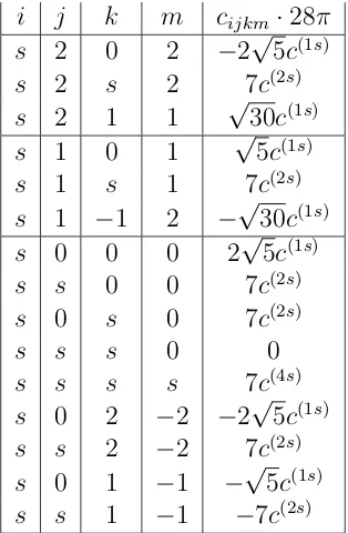
have angular momentum zero in the radial case). This is a consequence of the Perron-Frobenius theorem which holds under weak assumptions on V. The construction of these potentials is based on a new fact about the maxima of half-integer Bessel functions which is discussed in the appendix to Chapter V.

The macroscopic persistence of boundary conditions

In Chapter VI, we describe joint work with Rupert L. Frank and Barry Simon in which we consider a zero-temperature and low-density version of the BCS theory in which particles are conned to a domain Ω⊂ Rd _{and are subjected} to a weak external eld W : Ω → R. Clearly, the model is then no longer

(29)

First, the system states are now described by an operator 0 ≤ Γ ≤ 1 on

L2_(Ω)_⊕_L2_(Ω) _{of the form}

Γ = γ α

α 1−γ

!

,

which is no longer a multiplication operator in Fourier space. Here γ and α are operators on L2_(Ω) _{and we can describe them via their operator kernels}

γ(x, y) and α(x, y).

We introduce a small parameter h > 0 that describes the ratio between the

microscopic and macroscopic lengthscales. The BCS energy is dened as

E_µBCS(Γ) = Tr[(−h2∆Ω+h2W −µ)γ] + Z Z

Ω×Ω

V

x−y h

|α(x, y)|2dxdy. (2.10) Here −∆Ω is the Dirichlet Laplacian on Ω; it indicates the connement of

the particles to the domain Ω. The bounded function W : Ω → R describes

the external potential; it is weak because it comes with the h2 prefactor. We emphasize that there is no entropy term in (2.10) because we consider the system at zero temperature.

We will consider this energy at choices of the chemical potential µ ∈ R that

correspond to small particle density. The physical picture that we have in mind is the following: the system will be composed mostly of tightly bound fermion pairs. At low density, these pairs are on average far apart and thus look like bosons to one another. Since we are at zero temperature, the pairs should then form a Bose-Einstein condensate. In analogy to the derivation of Ginzburg-Landau theory in the previous section, we can then derive an eective Gross-Pitaevskii theory describing the condensate of fermion pairs. The fact that BCS theory can be used to describe this physical regime was noticed in the early 80s and is commonly called the BCS-BEC crossover. To implement the idea of tightly bound fermion pairs, we make the key as-sumption that the potentialV is indeed strong enough to form a bound state. Assumption 2.2.3. V :Rd→R is such that−Eb := inf spec(−∆Rd+V)<0.

(30)

below indeed corresponds to low density). The GP energy is dened similarly to the Ginzburg-Landau energy from the previous section as

EGP

D (ψ) :=

Z

1 4|∇ψ|

2_{+ (}_W ₋_D_)|_ψ_|2₊_g_|_ψ_|4

dx,

where D ∈ R and g > 0 are parameters. As before, D represents some

ad-missible class of BCS states Γ that renders the minimization problem EBCS µ well-dened. The detailed denition of D can be found in Chapter VI.

Theorem 2.2.4. Assume that Ω⊂Rd _{is a bounded Lipschitz domain and that} V satises the assumption above. Then, there exists cΩ >0 so that, as h ↓0,

we have

inf Γ∈DE

BCS

−Eb+Dh2(Γ) =h

4−d _inf ψ∈H1

0(Ω)

EGP

D (ψ) +O(h4

−d+cΩ₎_, _(2.11) for some explicit g >0.

We remark that the constantcΩ >0in the error term depends on the regularity

of Ω. For example, one can choosecΩ = 1−ε for any ε >0 if Ωis convex.

This theorem is not the rst in this context. Similar results were proved on the torus [94] and on the full space with bounded W [28]. A time-dependent analogue was proved in [91]. The dierence between all of these results and ours is that they consider a system without boundary. We consider instead a system with a sharp boundary, modeled by the Dirichlet condition.

On the right-hand side of (2.11), observe that the minimization takes place over the Sobolev space H1

0(Ω). In other words, the Dirichlet boundary

condi-tions are preserved under the limit h ↓ 0. This is not a priori clear. We are

integrating out microscopic scales to arrive at the GP energy and one might think that the boundary condition is a subleading eect as one integrates out small scales. The result says that the boundary in fact plays a role on the macroscopic scale to leading order. To see that this is a subtle question, we mention that de Gennes [58] predicted that, at positive temperature and den-sity, the sharp boundary conditions should be forgotten (i.e. a Dirichlet BCS energy should yield a Neumann Ginzburg-Landau energy).

(31)

2.3 The entanglement inherent to fermionic states

In Chapter VII, we describe a recent result concerning the entropy of the reduced density matrices of any permutation-invariant quantum state. These entropies can be viewed as a way to quantify the entanglement that is inherent to a quantum state.

To make this more precise, let us dene the quantities under consideration. We consider the many-body Hilbert spaceNN

m=1C

d_{, where} _d_{is the dimension} of the one-body Hilbert space. We will take d ≥ N which is necessary for having fermionic states. (We have d ≥N e.g. for a tight-binding model of N spin-polarized electrons hopping ond lattice sites.) Given any quantum state ρN on the many-body Hilbert space, we obtain its k-body reduced reduced density matrix by tracing out N −k of the particles, i.e.,

γk= Trk+1,...,N[ρN].

Here we use the convention for the partial trace that givesTr[γk] = Tr[ρN] = 1. We are interested in the following entropies

Sk :=S(γk) :=−Tr[γklogγk].

These entropies quantify the entanglement of the state ρN with respect to the Hilbert space decomposition

N

O

m=1

Cd ₌ k

O

m=1

Cd_⊗ N−k

O

m=1

Cd_,

i.e., they quantify the extent to which k particles are entangled with the re-maining N −k particles in the state ρN. We are interested in nding lower bounds on the entropies Sk. In other words, we are interested in nding the states that are the least entangled in this sense.

For bosonic states, one can make allSk = 0. This is achieved by taking ρN to be a pure condensate wave function, namely

ρN =|φ⊗Nihφ⊗N|.

Indeed, then we have for everyk thatγk =|φ⊗kihφ⊗k| is still a pure state and

so its entropy vanishes.

(32)

in this sense. A natural question is then which fermionic states minimize the entropies Sk. By concavity of the entropy, one may restrict to pure fermionic states |ΨNihΨN|.

In 1976, Coleman [39] solved this problem in the k = 1 case.

Theorem 2.3.1 (Coleman). S(γ1) ≥ logN and the minimum is achieved if ΨN is a Slater determinant.

Coleman's result was generalized to the following conjecture by Carlen, Lieb and Reuvers (CLR) in 2016 [33].

Conjecture 2.3.2. S(γ2)≥ log N₂ and the minimum is achieved if ΨN is a Slater determinant.

The fact thatS(γ2) = log N₂

for Slater determinants follows from an elemen-tary computation. CLR also put forward a weaker, asymptotic form of their conjecture thatS(γ2)≥2 logN +o(1) asN → ∞. They prove in their paper

that

S(γ2)≥logN +o(1) (2.12)

by using a strengthened form of the strong subadditivity of the quantum en-tropy. (Alternatively, this fact can be proved by using Yang's bound on the largest eigenvalue of γ2, as is also mentioned in [33].)

One of the observations put forward in Chapter VII are general properties of the map k 7→Sk that yield an improvement of (2.12) as a corollary.

Theorem 2.3.3. Let γk be the k-body density matrix of any permutation-invariant pure state |ΨNihΨN|. Then the map k 7→Sk has the following prop-erties.

(i) Monotonicity. For every 1≤k≤ N

2 −1,

Sk≤Sk+1. (2.13)

(ii) Concavity. For every 2≤k ≤N−1,

Sk≥

Sk+1+Sk−1

(33)

These properties follow directly from applications of the monotonicity of the relative entropy and the symmetry property Sk = SN−k which holds for any permutation-invariant state. (Note that if ΨN is a fermionic wave function, then |ΨNihΨN| is a permutation-invariant state.)

Combining the monotonicity property with Coleman's theorem yields

S2 ≥S1 ≥logN,

so as a corollary we obtain a new proof of (2.12).

Chapter VII contains the proof of this result as well as another theorem that establishes the bound S(γ2) ≥2 logN + log(d−N). This bound also follows

from Yang's bound on ther largest eigenvalue of γ2, but we give an entropic

proof of it that is is inspired by a joint work on approximate quantum cloning with Mark M. Wilde [121]. We note that the boundS(γ2)≥2 logN+ log(d−

N) implies the conjecture by CLR if d−N =O(1).

(34)

C h a p t e r 3

NEW ANOMALOUS LIEB-ROBINSON BOUNDS IN

QUASI-PERIODIC XY CHAINS

David Damanik, Marius Lemm, Milivoje Lukic and William Yessen

3.1 Introduction

Relativistic systems are local in the sense that information propagates at most at the speed of light. In their seminal paper [124], Lieb and Robinson found that non-relativistic quantum spin systems described by local Hamiltonians satisfy a similar quasi-locality under the Heisenberg dynamics. Their Lieb-Robinson bound and its recent generalizations [97, 138] implies the existence of a light cone |x| ≤ v|t| in space-time, outside of which quantum correlations

(concretely: commutators of local observables) are exponentially small. In other words, the LR bound shows that, to a good approximation, quantum correlations propagate at most ballistically, with a system-dependent Lieb-Robinson velocity v.

About ten years ago, the general interest in LR bounds re-surged when Hast-ings and co-workers realized that they are the key tool to derive exponential clustering, a higher-dimensional Lieb-Schultz-Mattis theorem and the cele-brated area law for the entanglement entropy in one-dimensional systems with a spectral gap [99, 97, 98]. These results highlight the role of entanglement in constraining the structure of ground states in gapped systems and yield many applications to quantum information theory, e.g. in developing algorithms to simulate quantum systems on a classical computer [29, 13].

In this paper, we announce and sketch the rigorous proof of a new kind of anomalous (or sub-ballistic) Lieb-Robinson bound for an isotropic XY chain in a quasi-periodic transversal magnetic eld. The LR bound is anomalous in the sense that the forward half of the ordinary light cone is changed to the region |x| ≤v|t|α for some ₀_{< α <}₁.

Previous study has focused on the dependence of the Lieb-Robinson velocityv on the system details [138], with particular interest in the case v = 0, since it

(35)

a logarithmic light-cone was obtained for long-range, i.e. power-law decaying, interactions. The anomalous LR bound we nd yields a qualitatively completely dierent, anomalously slow many-body transport.

We expect that if one has an anomalous LR bound for a system with a spec-tral gap, the arguments of [99, 138] will yield anomalously strong exponential clustering (see the discussion after Def. 1).

We actually have an exact characterization of the values of α for which the anomalous LR bound holds, namely whenever αexceeds α+_u, the upper trans-port exponent of the one-body discrete Schrödinger operator with potential given exactly by the quasi-periodic eld. Thanks to extensive study, there exist both rigorous and numerical upper and lower bounds on α+

u [3, 42, 43, 45, 46, 51, 52].

We mention that quasi-periodic sequences serve as models for one-dimensional quasi-crystals and their sometimes exotic transport properties. Especially the discrete one-body Schrödinger operator with Fibonacci potential, see (3.5), has been considered [113, 143, 3, 35, 165, 86, 166, 49, 46, 51, 52, 44, 43, 45]. Quasi-periodic spin chains (in particular with Fibonacci disorder) have also been studied extensively, with a focus on spectral properties and critical phenomena [21, 22, 23, 59, 100, 36, 153, 130].

While we give the full statements below, we only give a rough sketch of the proof; a detailed version will appear elsewhere [48].

3.2 Setup and main result

For any integer N, we consider the isotropic XY chain dened by the Hamil-tonian

HN =− N−1 X

x=1

σ_x1σ_x1₊₁+σ_x2σ_x2₊₁+

N

X

x=1

hxσ3x, (3.1) whereσ1_{, σ}2_{, σ}3 are the usual Pauli matrices. We scaled out the usual_J factor

in front of the rst term and chose zero boundary conditions for convenience. For deniteness, we let hx be the Fibonacci magnetic eld

hx =λχ[1−φ,1)(xφ+ω mod 1), (3.2)

whereλ >0is a coupling constant, ω∈[0,1)is an arbitrary phase oset, and

φ is the inverse of the golden mean, i.e. φ=

√ 5−1

(36)

The Fibonacci eld (3.2) is prototypical in the study of one-dimensional quasi-crystals, but in fact φ can be replaced by an arbitrary irrational number in

(0,1)here (Sturmian class); compare [113, 143, 154, 17, 43]. We letOxdenote the set of observables at site x, which is of course just the set of Hermitian

2×2matrices, and for an observable A, we let

A(t)≡eitHN_Ae−itHN (3.3)

be its image under the Heisenberg evolution after time t. Note that A(t)

implicitly depends on N as well.

Denition 3.2.1 (anomalous LR bound). We say that LR(α) holds if there

exist positive constants C, ξ, v such that for all integers x, x0, N with 1≤ x < x0 ≤N and all times t >0, the bound

k[A(t), B]k ≤CkAkkBke−ξ(|x−x0|−vtα) (3.4) holds for all observables A∈ Ox and B ∈ Ox0.

Let us make a few remarks about this: Firstly, the usual Lieb-Robinson bound corresponds to LR(1) and is known to hold by general considerations [124].

When comparing LR(α) with LR(1) in the particularly relevant regime of

small times, it is important to keep in mind that|x−x0| ≥1by denition and

consequently |x−x0|1/α_>_|_x₋_x0_| _for ₀_{< α <}₁_{. Hence, for xed}_t_,_LR₍_α₎_is

eective at smaller distances than LR(1). Secondly, (3.4) can be extended to

a much wider class of observables, provided that their supports are a non-zero distance apart [48, 50]. Thirdly, we emphasize that the constants above do not depend on the system size N, so that the estimate (3.4) is stable in the thermodynamic limit N → ∞. Finally, as mentioned in the introduction, if

one can proveLR(α)for a system with a spectral gap, we expect that

ground-state correlations will decay anomalously fast, i.e. the usual exponential decay in d(X, Y) is replaced by decay in d(X, Y)1/α _{(see e.g. Theorem 2 in [138]).} Essentially, this should follow from the proofs in [99, 138], by using LR(α)

instead of LR(1), which only changes the optimization problem in the time

cuto parameter (called s in [138]). Our rst main result is:

(37)

As mentioned in the introduction, we actually have a characterization of the values of α for which LR(α) holds for all λ > 0. This characterization is in

terms of the upper transport exponentα+

u of the one-body discrete Schrödinger operator h with Fibonacci potential. It acts on a square-summable sequence

{ψx}x≥1 by

(hψ)_x=ψx+1+ψx−1+hxψx, (3.5) with ψ0 ≡ 0 and hx given by (3.2). α+u is then the propagation rate of the fastest part of an initially localized wave-packet. Since exponential tails cannot be evaded in quantum mechanics, α+

u is, roughly, the largest exponent β for which the probability of an initially localized wavepacket to travel a distance tβ _{in time}_t _{is not exponentially small.}

More formally: For any integer x≥1 and any positive real number β, let P(x, t) = X

x0_>x

|hδx0|e−ith|δ1i|2, (3.6)

R+(β) =−lim sup

t→∞

logP(tβ_{, t}₎

logt . (3.7)

Then, we dene

α+_u = sup

β≥0

R+(β)<∞ . (3.8)

Note that α+

u = α+u(λ). We mention that αu+ is just one of several transport exponents commonly associated to anomalous one-body dynamics [51, 52], but as it turns out it is the only one relevant for LR bounds.

As anticipated before, we have the following characterization:

Theorem 3.2.3. Let λ > 0. If α > α+_u, then LR(α) holds. Conversely, if

α < α+_u, then LR(α) does not hold.

In words, LR(α)is a precise way to state that tails are exponentially decaying

beyond a modied light-cone of the form|x| ≤vtα, and our theorem states that this is true for α > α+_u and false for α < α_u+. In fact, the second statement holds for completely general transversal magnetic elds (e.g. periodic ones, whereα+

(38)

We also obtain an explicit expression for the LR velocity v, see (38) in [48]. Appropriately, v is a decreasing function of α.

Let us discuss α+_u from a quantitative viewpoint. Since Theorem 2 holds for arbitrary coupling constant λ > 0, we see that the restriction to λ ≥ 8 in

Theorem 1 is due to the fact that we do not know rigorously that α+

u < 1 for all λ > 0 (we do know that α+

u > 0 for all λ > 0 [46]). We emphasize that estimating α+

u is only a problem of one-body dynamics however, which is simpler from both a theoretical and a numerical standpoint. A rough nu-merical study we conducted suggests that α+

u < 1 also holds for 0 λ < 8, and we think it would be interesting to pursue the numerical aspects further. Moreover, explicit rigorous upper and lower bounds for α+_u exist [51, 52, 45]. Asymptotically, they behave like 2 log(1+φ)

logλ for largeλ and they can be used to obtain quantitative estimates, such as

0.1< α+_u <0.5

for all 12 ≤ λ ≤ 7,000. We stress the upper bound by 0.5 because the

par-ticular case α+

u = 0.5is sometimes called diusive transport and not assigned the anomalous label.

3.3 Sketch of proof

Following [125], we map the XY chain to free fermions via the Jordan-Wigner transformation. That is, we introduce the spin raising and lowering operators

S± = 1

These operators satisfy the CAR and allow us to rewrite the Hamiltonian as

HN =

Here,hN is the operatorhdened in (3.5), but with a zero boundary condition at site N + 1. At this stage, HN can be diagonalized by a standard Bogoli-ubov transformation. One nds the following formula [96] for the Heisenberg dynamics (3.3) of the fermion operators:

(39)

Denition 3.3.1. We say that LRfermi(α) holds if there exist positive

con-stants C, ξ, v such that for all integers x, x0, N with 1 ≤ x < x0 ≤ N and all times t >0, the bound

k[cx(t), B]k+k[c†x(t), B]k ≤CkBke

−ξ(|x−x0|−vtα₎

(3.11) holds for all observables B ∈ Ox0.

As we will see, (3.10) allows us to proveLRfermi(α)by controlling the one-body

transport created by h. This is not surprising, because (3.10) is an expression

of the fact that we are now describing free particles.

The problem that arises, though, is that the Jordan-Wigner transformation (3.9) is highly non-local, while a Lieb-Robinson bound is of course an inherently local statement. The key lemma, which is somewhat surprising at rst sight, however, says

Lemma 3.3.2. LRfermi(α) is equivalent to LR(α).

The point is that, as originally realized in [96] and adapted here to our pur-poses, inverting the non-local Jordan-Wigner transformation essentially just requires summing up fermionic LR bounds: By an iteration argument, which is based only on(AB)(t) =A(t)B(t)and the usual commutator rules, one can

show

k[S_x−(t), B]k ≤2

x

X

y=1

k[cy(t), B]k+k[c†y(t), B]k

(3.12)

for allB ∈ Ox0. By taking adjoints and using commutator rules, similar bounds hold for S_x−, S_x−S+

x, Sx+S

−

x and hence for all elements of the four-dimensional algebra of observables Ox. Assuming that LRfermi(α) holds, we now see that

LR(α) follows from (3.12) and the trivial, but important, fact that

x

X

y=1

e−ξ(|y−x0|−vtα) ∝e−ξ(|x−x0|−vtα).

(40)

To prove Theorem 2, thanks to Lemma 1, it remains to characterize the values ofαfor whichLRfermi(α)holds. We rst show thatα > αu+impliesLRfermi(α).

By (3.10) and the fact that cy and B commute fory < x0, we get

k[cx(t), B]k ≤ kBk N

X

y=x0

hδx|e−2ihNt|δyi

. (3.13)

Since spatial translation corresponds to a shift of the (anyway arbitrary) phase osetω, modulo some technical diculties, the right-hand side is equal to

N−x−1 X

y=x0₋_x₋₁

hδ1|e−2ihNt|δyi

(3.14)

and this expression is already quite similar to the denition of the outside probability in (3.6). This explains why we can apply techniques developed in [42, 51, 52, 45] to study the transport exponent α+

u to our situation. A rough outline of the by now standard approach reads:

(a) use Dunford's formula

hδ1|e−2ihNt|δyi=−

1 2πi

Z

Γ

e−itzhδ1| 1 −2hN −z

|δyidz

to express the time-evolution in terms of resolvents (Γ is a simple

posi-tively oriented contour around the spectrum of −2hN),

(b) bound matrix elements of resolvents in terms of transfer matrix norms, by studying individual solutions,

(c) bound transfer matrix norm by the exponentially decaying right-hand side in LRfermi(α), by studying the Fibonacci trace map.

However, the original results of [42, 51, 52, 45] do not translate directly to our situation. Firstly, the operator h lives on the half-line, while hN has a zero boundary condition at N + 1. This is a minor obstruction and can be

removed, for an upper bound, by one-rank perturbation theory on the level of resolvents.

(41)

solution we have found to this will not be presented here for the sake of brevity and instead we refer the interested reader to [48].

We now turn to the converse direction in Theorem 2. We prove the logically equivalent statement that LRfermi(α) implies α ≥ α+u. Using (3.10) and an appropriate trial state to bound the operator norm (see [48] for details), we obtain the key estimate

k[cx(t), S_x+0]k ≥

hδx|e−2ihNt_|_δx

0i

(compare with (3.13)). Thus, LRfermi(α) implies

hδx|e−2ihNt|δx0i≤Ce−ξ(|x−x

0_|−_vtα₎

for all 1 ≤ x ≤ x0 ≤ N and all t > 0. We take the limit N → ∞ to pass to

the half-line operator,

hδx|e−2iht|δx0i

≤Ce−ξ(|x−x

0_|−_vtα₎

(3.15) for all x, x0 ∈N and all t >0. Using this on denition (3.6) gives

P(tβ, t)≤ C 2

1−e−2ξe

−2ξ(tβ−v(t/2)α) _≤_Ce_˜ −ξtβ

whenever β > α. By denitions (3.7), (3.8) we conclude that β ≥ α+_u, so α≥α+_u.

3.4 The random dimer model

We explain why our method does not extend to yield an anomalous LR bound with power-law tails for the random dimer model [63]. The focus is on ideas here, for a detailed discussion see [48].

Recall the one-body discrete Schrödinger operator h from (3.5). In the

ran-dom dimer model, the potential hn is a random variable taking either of the two values ±λ, each with probability 1/2 say, but these values must always

occur in pairs (or dimers). The intuition, due to Anderson's work, that a one-dimensional disordered quantum system should exhibit localization is only al-most correct here: There exist critical energiesEc=±λfor which the transfer matrices across dimers commute and the system shows anomalous transport. As it turns out, the anomalous transport is so fast that α+

Mathematical Results on Quantum Many body Physics