Solid–liquid phase equilibrium for binary Lennard-Jones mixtures
Monica R. Hitchcock and Carol K. Halla)
Department of Chemical Engineering, North Carolina State University, Raleigh, North Carolina 27695-7905
~Received 8 January 1999; accepted 15 March 1999!
Solid–liquid phase diagrams are calculated for binary mixtures of Lennard-Jones spheres using Monte Carlo simulation and the Gibbs–Duhem integration technique of Kofke. We calculate solid– liquid phase diagrams for the model Lennard-Jones mixtures: argon–methane, krypton–methane, and argon–krypton, and compare our simulation results with experimental data and with Cottin and Monson’s recent cell theory predictions. The Lennard-Jones model simulation results and the cell theory predictions show qualitative agreement with the experimental phase diagrams. One of the mixtures, argon–krypton, has a different phase diagram than its hard-sphere counterpart, suggesting that attractive interactions are an important consideration in determining solid–liquid phase behavior. We then systematically explore Lennard-Jones parameter space to investigate how solid– liquid phase diagrams change as a function of the Lennard-Jones diameter ratio, s11/s22, and well-depth ratio,e11/e22. This culminates in an estimate of the boundaries separating the regions of solid solution, azeotrope, and eutectic solid–liquid phase behavior in the space spanned bys11/s22 ande11/e22for the case s11/s22,0.85. © 1999 American Institute of Physics.
@S0021-9606~99!51122-7#
I. INTRODUCTION
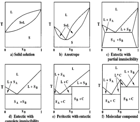
Successful design of melt crystallization processes de-pends upon knowledge of the equilibrium solid–liquid phase behavior of the mixture to be separated. Although mixture solid–liquid equilibrium can, in principle, be measured at any condition of interest, it would be useful to develop a theory that predicts mixture phase behavior based solely upon knowledge of the components’ molecular architecture and intermolecular forces. Such a theory should be able to predict the six types of binary solid–liquid phase diagrams introduced in 1977 by Matsuoka,1 a classification based on the analysis of nearly 1500 binary organic systems. The six types of binary solid–liquid phase diagrams are shown in Fig. 1; they include: solid solutions, azeotropes, eutectics with partial solid phase immiscibility, eutectics with com-plete solid phase immiscibility, peritectics with eutectics, and molecular compounds.
Our intent in this paper is to explore the range of Lennard-Jones parameters that will yield the phase diagrams characteristic of solid solutions, azeotropes, and eutectics with partial solid phase immiscibility. The solid phase in all of these phase diagrams is a substitutionally disordered solid solution, i.e., both species pack with the same crystalline structure and can substitute for one another in any order on the lattice. In future work we will examine the effect of Lennard-Jones parameters on solid–liquid equilibrium for cases in which the solid phase is an ordered crystal and the associated phase diagram contains either a peritectic with eutectic or a molecular compound.
Several workers have developed molecularly-based
theories of solid–liquid phase equilibria using simple mod-els, such as the hard-sphere model or the Lennard-Jones 12–6 potential model, in an effort to understand how mo-lecular size differences and interactions influence the phase behavior of a mixture. Cottin and Monson2developed a cell theory for binary solid solutions based on the early cell model of Lennard-Jones and Devonshire for single compo-nent solids. In this model, each molecule is assumed to move within the cage formed by its nearest neighbors. A cell is characterized by the identity of its central molecule and by the composition and geometrical arrangement of its nearest neighbors. Assuming that the product of the cell partition functions is equal to the configurational partition function, the solid solution free energy can be determined as a func-tion of composifunc-tion. The liquid solufunc-tion free energy can be obtained from an equation of state. Once the free energies of both phases are obtained, the convex envelope construction method is used to locate the solid–liquid phase envelope.
The cell theory has been applied to phase diagram cal-culations for both hard-sphere and Lennard-Jones binary mixtures. Cottin and Monson calculated phase diagrams for binary hard-sphere liquid mixtures coexisting with substitu-tionally disordered fcc ~Ref. 2! and several ordered3binary hard-sphere solids. Cottin and co-workers4,5showed that the cell theory is capable of predicting five of the six solid– liquid phase diagrams displayed in Fig. 1. The only type of phase diagram that the cell theory with the hard-sphere po-tential model does not predict is that for molecular com-pound formation. The fact that the hard-sphere model can generate five of the six known types of solid–liquid phase diagrams indicates that packing and molecular size differ-ences, which are the major consideration in a hard-sphere mixture, are the dominant factors in determining the shape of solid–liquid phase diagrams in real systems.
a!Author to whom correspondence should be addressed: electronic mail: [email protected]
11433
Cottin and Monson also calculated phase diagrams for binary Lennard-Jones liquid mixtures6 coexisting with sub-stitutionally disordered fcc binary Lennard-Jones solids. They calculated phase diagrams for argon–methane, argon– krypton, and krypton–methane, and compared them with ex-perimental results. They found that the shape of the phase diagram predicted by cell theory is similar to the shape of the phase diagram observed experimentally.
Another approach to calculating solid–liquid equilibria is density functional theory. In density functional theory, a crystalline solid is treated as if it were an inhomogeneous liquid.7There seem to be two main approaches to developing analytical expressions for the free energy of the solid: trun-cated perturbation expansions in which the excess free en-ergy is expanded about a uniform reference liquid,8,9 and nonperturbative effective liquid approximations in which the excess free energy of the nonuniform liquid ~crystalline solid!is approximated by the excess free energy of a uniform liquid evaluated at an effective density.10,11The liquid solu-tion free energy can be obtained from an equasolu-tion of state. As in the cell theory, once the free energies of both phases are obtained, the convex envelope construction method is used to locate the solid–liquid phase envelope.
Density functional theory has been applied to the calcu-lation of phase diagrams for hard-sphere and Lennard-Jones binary mixtures. Rick and Haymet,8,9Denton and Ashcroft,11 and Zeng and Oxtoby10 used density functional theory to calculate phase diagrams for binary hard-sphere liquid mix-tures coexisting with substitutionally disordered fcc hard-sphere solid solutions. Rick and Haymet, and Denton and Ashcroft also investigated the range of stability for several ordered binary hard-sphere solid solutions coexisting with a liquid, where the composition of each phase was fixed at x
50.5. The nonperturbative theories ~Denton and Ashcroft, Zeng and Oxtoby! give more accurate results than the per-turbative theories~Rick and Haymet!. As was the case with the cell theory, the density functional theory applied to bi-nary hard-sphere mixtures shows that size differences alone can determine the shape of the phase diagram. Density func-tional theory is not as successful as cell theory at predicting phase behavior in binary Lennard-Jones systems. Rick and Haymet used density functional theory to calculate solid– liquid phase diagrams for binary Lennard-Jones mixtures of argon–methane, argon–krypton, and krypton–methane, and compared them with experimental results. Of the three sys-tems, they were only able to predict the shape of the krypton–methane phase diagram correctly.
It is common practice to test molecularly-based theories, such as cell theory and density functional theory, with mo-lecular simulation data. Since momo-lecular simulations are ex-act calculations for a given molecular model, they provide a direct test of theoretical approximations. The approach taken in most simulations of solid–liquid phase equilibrium in-volves calculating the free energy of each phase separately and then determining the coexistence curve using the convex envelope construction method. Since the free energy cannot be directly measured in a simulation, thermodynamic inte-gration techniques are often used. In thermodynamic integra-tion, the free energy of a phase is calculated by numerically integrating along a reversible path from a reference state to the desired state. This integration requires simulation data at many intermediate state points. The liquid phase free energy can be calculated by thermodynamic integration from the ideal gas reference state. The solid phase free energy cannot be determined by thermodynamic integration from the ideal gas state because this path crosses a first-order transition, where appreciable hysteresis may occur, and is irreversible.12 There are, however, other free energy reference states that can be used. Frenkel and Ladd13have used the Einstein crys-tal as a reference state to calculate the free energy of a hard-sphere solid via thermodynamic integration. An Einstein crystal consists of regularly-spaced molecules that are held in place on a lattice by the repulsive forces between their near-est neighbors.14 Eldridge et al.15–17 have used Frenkel and Ladd’s Einstein crystal integration method to calculate the free energies of binary hard-sphere solids with ordered phases such as AB, AB2, and AB13. Frenkel and Ladd’s integration method is not well-suited for substitutionally dis-ordered solid phases, i.e., solid solutions, because there are relatively small free energy differences between the real mix-ture and the Einstein reference mixmix-ture.18
Other thermodynamic integration approaches have been taken for solid–liquid equilibrium calculations when the solid is a disordered crystal. Kranendonk and Frenkel18,19 developed two methods for calculating the free energies of disordered fcc binary hard-sphere solid solutions using the free energy of a pure hard sphere fcc solid, as calculated by Frenkel and Ladd, as the reference state. In one method, they construct a reversible path from the pure hard-sphere fcc solid reference by fixing the density and diameter ratio and varying the composition from unity to the composition of the hard-sphere mixture using particle insertion techniques. In a
second method, they construct a reversible path by fixing the density and composition and varying the diameter ratio from unity to the diameter ratio of the hard-sphere mixture. Kofke20 introduced another thermodynamic integration method for calculating solid–liquid coexistence for cases in which the solid is a disordered binary hard-sphere fcc solid solution. This method utilizes semigrand canonical ensemble simulations21,22in which the number of molecules, tempera-ture, pressure, and species fugacity fractions are fixed and the density and composition are allowed to vary. Kofke used semigrand canonical simulations to generate composition versus fugacity fraction data for several solid phase iso-therms. Using this data and the chemical potential of one of the pure species as a reference ~taken from the data of Hoover and Ree!,23 Kofke integrated the semigrand canoni-cal fundamental equation to canoni-calculate the species chemicanoni-cal potential as a function of fugacity fraction for each isotherm. The chemical potential versus fugacity fraction curve for the liquid phase was obtained from a hard-sphere equation of state. Since the species chemical potentials and fugacity frac-tions must be equal at equilibrium, phase coexistence could be found for each isotherm by determining the intersection of the chemical potential versus fugacity fraction curves.
Using cell theory and the molecular simulation tech-niques described above, several workers have determined the range of size ratios in binary hard-sphere mixtures that yield the various types of phase diagrams. Table I lists hard-sphere diameter ratios that produce solid–liquid phase diagrams of the solid solution, azeotrope, and eutectic types, along with the diameter ratio boundaries between these three types. These substitutionally disordered solids are generally stable with respect to phase separation at diameter ratios greater than 0.85. For lower diameter ratios substitutionally ordered
solids are stable. Table II gives the range of diameter ratios over which the structures, AB, AB2, and AB13are stable in hard-sphere mixtures.
To our knowledge, the only simulation study of solid– liquid equilibrium in binary Lennard-Jones mixtures is that of Vlot et al.24 who calculated solid–fluid phase diagrams for symmetric~equal diameters,s115s22; equal attractions, e115e22) binary Lennard-Jones mixtures using a combina-tion of molecular simulacombina-tion and theory. Cross interaccombina-tions between the components were defined ase125e
A
e11e22and s125s(s111s22)/2 where the parameters e and s represent deviations from the Lorentz–Berthelot mixing rules.25 They used a variety of thermodynamic integration and particle in-sertion techniques to calculate free energies. The solid phase free energy was calculated using the Einstein crystal refer-ence state,26 the liquid phase free energy was calculated us-ing the f g samplus-ing method,27,28and the gas phase free en-ergy was calculated using Widom’s test particle insertion.29 The excess free energy versus composition data for all of the phases was fit with a two-parameter Redlich–Kister polynomial.30The convex envelope construction method was used to determine the temperature versus composition phase diagrams.In the simulation techniques that we have discussed thus far, phase equilibrium is calculated indirectly in that many simulations must be conducted at uninteresting state points in order to get one coexistence point. Prior to 1987, direct simulation of phase equilibrium was considered to be too computationally expensive because the presence of an inter-face requires the system to contain an unusually large num-ber of particles. Then in 1987, Panagiotopoulos31introduced the Gibbs ensemble method for direct simulation of phase coexistence in single component fluids and in 1988, extended the method to phase coexistence in multicomponent mixtures.32 In this method the coexisting phases are simu-lated independently, so as to remove the interface, yet are essentially coupled together in order to satisfy the criteria of phase equilibrium: equal temperatures, pressures, and spe-cies chemical potentials. These conditions are satisfied by simulating each phase at the same temperature and pressure, and performing particle exchanges between the phases to maintain chemical potential equality. The Gibbs ensemble method has been widely used to study vapor–liquid and liquid–liquid phase equilibria. However, because a large
TABLE I. Diameter ratios for binary hard-sphere mixtures that exhibit solid–liquid phase diagrams of the solid solution, azeotrope, and eutectic types. All of the solid phases are substitutionally disordered solid solutions except for eutectics with complete immiscibility, in which case the solid phases contain only one component.
Phase diagram Cell theorya
Thermodynamic integrationb
Semigrand Monte Carloc
Solid solution 0.95, 0.97 0.95 0.95
Solid solution/azeotrope boundary 0.9425
Azeotrope 0.9, 0.92, 0.93, 0.94 0.9, 0.92 0.9, 0.93
Azeotrope/eutectic boundary 0.875
Eutectic with partial immiscibility 0.85 0.85
Eutectic with complete immiscibility 0.62, 0.73, 0.8
a
Reference 4. bReference 19. cReference 20.
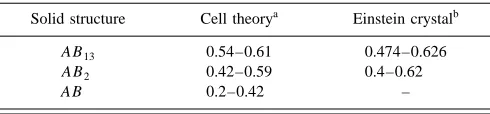
TABLE II. Range of diameter ratios at which binary hard-sphere mixtures form stable substitutionally ordered solid solutions of the types AB13, AB2, and AB.
Solid structure Cell theorya Einstein crystalb
AB13 0.54–0.61 0.474–0.626
AB2 0.42–0.59 0.4–0.62
AB 0.2–0.42 –
a
number of successful transfers of particles between each phase are required for chemical potential equilibration,33the Gibbs ensemble method is not an efficient method for study-ing solid–liquid phase equilibrium.
Inspired by the Gibbs ensemble method, Kofke34,35 in-troduced the Gibbs–Duhem integration technique for direct simulation of phase equilibria. As in the Gibbs ensemble method, two or more coexisting phases are simulated inde-pendently at the same temperature and pressure. However, instead of using particle exchanges, Kofke maintains chemi-cal potential equality in each phase by integrating along the Clapeyron equation for coexistence during the simulations. Eliminating the need for particle transfers between phases makes the Gibbs–Duhem integration method well-suited for calculating phase equilibrium for cases in which one of the phases is a solid. The Gibbs–Duhem integration simulation approach has been used to tackle a number of multicompo-nent, multiphase equilibrium problems, including: finding the triple point of the Lennard-Jones fluid,36,37determining the melting line of C60,38and calculating phase diagrams for colloids in polymer solution39 and for polymer-induced pro-tein precipitation.40 In each case the appropriate Clapeyron differential equation is derived and an initial coexistence condition is obtained from theory, experimental data, or a Gibbs ensemble Monte Carlo simulation.
In this paper, we combine Kofke’s Gibbs–Duhem inte-gration technique with semigrand canonical Monte Carlo simulations to calculate solid–liquid phase diagrams for bi-nary Lennard-Jones mixtures. To our knowledge, these are the first direct simulations of solid–liquid equilibrium in bi-nary Lennard-Jones mixtures.
We calculate solid–liquid phase diagrams for binary Lennard-Jones mixtures with diameter ratios ranging from 0.85 to 1 and attractive well-depth ratios ranging from 0.45 to 1.6, at a reduced pressure equivalent to 1 atm. We deter-mine the cross-species interaction parameters by using the Lorentz–Berthelot25 mixing rules. The solid–liquid equilib-rium line is calculated for each mixture by numerically inte-grating the Clapeyron differential equation for binary mix-ture phase equilibria at constant pressure. The initial condition for the integration is that of a single component Lennard-Jones liquid in equilibrium with a single component Lennard-Jones fcc crystalline solid at atmospheric pressure. The coexistence properties at subsequent integration points are determined by semigrand canonical Monte Carlo simula-tions ~constant temperature, pressure, total number of mol-ecules, and fugacity fraction!of the liquid and the fcc solid phases.
Highlights of our simulation results are the following. In a test of the cell theory predictions for model argon– methane, argon–krypton, and krypton–methane systems, we found that cell theory can qualitatively predict the shape of phase diagrams for Lennard-Jones mixtures. Comparison of our simulation results for the argon–krypton Lennard-Jones system with hard-sphere results at the same diameter ratio indicated that the presence of attractive interactions can change the type of phase diagram observed from azeotrope
~hard-sphere! to solid solution ~Lennard-Jones!. This sug-gested that attractive interactions are an important factor in
determining the type of solid–liquid phase behavior ob-served and prompted a more thorough investigation of the effect of variations in well-depth ratio on solid–liquid phase diagrams. We simulated 56 binary Lennard-Jones mixtures over the range of parameters listed above to determine how solid–liquid phase diagrams change as a function of diam-eter ratio and well-depth ratio. We found that for well-depth ratios of unity ~equal attractions among species! phase be-havior indicative of azeotropes and eutectics is observed for diameter ratios ranging from 0.85 to 1. We then varied the well-depth ratio of the mixtures at several constant diameter ratios and observed transitions from azeotrope to solid solu-tion, from azeotrope to eutectic, and from solid solution to simple peritectic. Using our simulation results, we are able to map out the boundaries separating regimes of solid solution, azeotrope, and eutectic solid–liquid phase behavior in the space spanned by the Lennard-Jones diameter ratio and well-depth ratios.
The remainder of the paper is organized as follows. Sec-tion II reviews the Gibbs–Duhem integraSec-tion method and gives details of how we applied the technique to our study of binary solid–liquid mixture equilibrium. In Sec. III, the simulation results are presented and discussed. A brief sum-mary and further discussion are given in Sec. IV.
II. METHOD
In this section we describe how we calculated solid– liquid equilibria in binary Lennard-Jones mixtures using the Gibbs–Duhem integration method. We begin by presenting a brief overview of the Gibbs–Duhem integration method. We then discuss our procedures for determining an initial coex-istence condition and integrating the Clapeyron equation. Fi-nally, we describe the details of the semigrand ensemble simulations used throughout the integration procedure.
In the Gibbs–Duhem integration method,34,35,41 phase coexistence is determined by numerically integrating the Clapeyron differential equation appropriate to the system of interest. Clapeyron equations describe how field variables
~variables that must be equal among coexisting phases! change along the phase equilibrium line. The Clapeyron equation for equilibrium between a binary solid mixture and a binary liquid mixture at constant pressure is35
db
dj25
~x2l2x2s!
j2~12j2!~hl2hs!, ~1!
wherebis the reciprocal temperature, 1/kT, with k the Bolt-zmann constant and T the absolute temperature, j2 is the fugacity fraction of species 2, j2[fˆ2/(fˆi, with fˆi, the fugacity of species i in solution, x2 is the mole fraction of species 2, h is the molar enthalpy, and the superscripts l and
s denote the liquid and solid phases, respectively. The
A. Initial condition
We need an initial coexistence condition before we can begin a Gibbs–Duhem integration calculation of solid–liquid equilibrium in a binary mixture. A good choice is the solid– liquid equilibrium condition for either of the pure components.35 Since the slope of the integrand in Eq.~1! is undefined for pure components (j250, x250 and j251,
x251), we instead estimate it using the limiting case of infinite dilution. Here we follow Mehta and Kofke,42 who used the infinite dilution case to start their Gibbs–Duhem integration calculations of vapor–liquid equilibria in binary mixtures.
Consider the case of pure species 1 solid–liquid coexist-ence. We can estimate (db/dj2)x250 by supposing that the real mixture displays ideal solution behavior at the limit of infinite dilution of species 2. With this assumption, the abun-dant component ~species 1!in the ideal solution follows the Lewis Randall rule
fˆ15x1f1, ~2!
while the dilute component~species 2!obeys Henry’s law
fˆ25x2H2, ~3!
where fˆ1 and fˆ2are fugacities of species 1 and 2 in solution,
f1is the fugacity of pure component 1 at the temperature and pressure of the mixture, and H2 is the Henry’s law constant for species 2. Letting x1→1 and x2→0, the fugacity fraction of species 2 becomes, j25x2H2/ f1. After making these substitutions into Eq. ~1!we get
db
dj2
U
x250
5 fˆ2/H2
l2fˆ
2/H2 s
~x2H2/ f1!~12x2H2/ f1!~hl2hs!, ~4!
which, after simplification, leads to
db
dj2
U
x250
5f1~1/H2
l2
1/H2s!
~hl2hs! . ~5!
This gives us an estimate of the integrand at the initial condition of j250 and melting temperature, T1, of pure species 1.
We can calculate all of the quantities on the right-hand side of Eq. ~5! with an NPT~constant number particles, N, pressure, P, and temperature, T!simulation of pure species 1. The molar enthalpy of each phase is h5
^
u1Pv&
NPT, whereu is the configurational energy of the system and the
brack-ets,
^ &
NPT, denote an NPT ensemble average. The quantityf1/H2 is given by42
f1
H2
5
^
exp~2bDu1→2!&NPT, ~6!whereDu1→2is the exchange energy associated with switch-ing a particle from species 1 to 2. The exchange energy,
Du1→2, can be obtained by conducting trial identity switches during the simulation. A trial identity switch con-sists of randomly selecting a particle and calculating the
en-ergy that would result if we were to switch the particle from species 1 to species 2. This is done without actually changing the particle’s identity.
B. Integration
Once we have an initial coexistence condition, we can begin the Gibbs–Duhem integration series using a predictor–corrector algorithm to integrate Eq. ~1! over the entire range of fugacity fractions,j250 toj251. Stepping to the next fugacity fraction, (j2)1, from the initial data point, the next reciprocal temperature, b1, can be estimated using the trapezoid-rule predictor formula
b1(0)5b01@~j2!12~j2!
0#F~b0,~j2!0!, ~7! where the ‘‘0’’ superscript indicates that b1(0) ~a predicted value!is our zeroth iteration attempt at finding the reciprocal temperatureb1, (j2)0andb0are the initial fugacity fraction and reciprocal temperature, respectively, and F is the right-hand side of Eq. ~1!evaluated at the initial condition. Once b1
(0) is estimated at the given fugacity fraction (j2) 1, two semigrand canonical (NPTj2) Monte Carlo simulations~one for the liquid phase and one for the solid phase! are con-ducted in order to equilibrate the configurations and to cal-culate the enthalpies and mole fractions at the new state point. ~Details of the NPTj2 simulations will be given in Sec. II C.!
After each phase is equilibrated we refine our estimate for b1 with the trapezoid-rule corrector
b1(1)5b01@~j2!12~j2!0# 2 @F1
(0)~b 1 (0)
,~j2!1!
1F0~b0,~j2!0!#, ~8!
where the subscripts ‘‘0’’ and ‘‘1’’ denote the initial and current conditions, respectively, and F1(0) is calculated from simulation averages of the enthalpies and mole fractions at b1
(0)and (j2)
1. After the reciprocal temperature is corrected, two NPTj2 simulations, one for each phase, are started si-multaneously and running averages of the compositions and enthalpies are calculated. Each simulation is paused periodi-cally and the running averages from the simulations to that point are used to calculate F1(i) and correct the reciprocal temperature to obtain the (i11)th estimate, b1(i11). This pattern continues until the temperature estimate stops vary-ing within a specified tolerance. A final production segment of simulations are run at the temperature determined from the corrector segment to obtain the final average enthalpies and mole fractions for the coexistence point.
bn11 (0) 5
bn2112@~j2!n112~j2!n#Fn~bn,~j2!n!, ~9!
bn11 (i11)5b
n211
@~j2!n112~j2!n# 3 @Fn11
(i) 1
4Fn1Fn21#,
~10! and the modified Adams predictor–corrector43 is used once three or more state points are known,
bn11 (0) 5b
n1
@~j2!n112~j2!n#
24 @55Fn259Fn21
137Fn2229Fn23#, ~11!
bn11 (i11)5b
n1
@~j2!n112~j2!n# 24 @9Fn11
(i) 119F n
25Fn211Fn22#. ~12! In these sets of equations the predictor is listed first. The subscripts denote the coexistence conditions determined from simulations with (n11) being the current simulation and the superscripts denote the iterations of the corrector for the current coexistence point. We mapped the entire tem-perature versus composition phase diagram by repeating the predictor–corrector algorithm fromj250 toj251.
C. Simulations
The enthalpies and mole fractions needed as input to the integration of Eq.~1!are obtained from semigrand canonical
~constant NPTj2) Monte Carlo computer simulations.22 In this work, all simulations were run with a system size of 500 particles at a reduced pressure equivalent to 1 atm. The tem-perature and fugacity fraction were varied according to the values specified by the Gibbs–Duhem integration predictor– corrector. There are three types of Monte Carlo trial moves in semigrand canonical simulations: particle displacements, volume change moves, and particle identity exchanges. The particle displacements and volume change moves are con-ducted just as they are in a standard NPT simulation.44In the particle identity exchange moves, a particle is selected at random and given a trial species identity switch. The identity switch is accepted according to the ratio of the species fugac-ity fractions,j1andj2. The overall acceptance probability42 for the moves in the NPTj2 ensemble is min@1,exp(L)# where
L52b~Utrial2Uold!2bP~Vtrial2Vold!
1N lnV
trial Vold1m ln
j2
12j2. ~13!
In Eq. ~13!, Utrial and Uold, and Vtrialand Vold are the con-figurational energies and volumes of the trial and existing states, respectively, m511 if the trial identity switch is from species 1 to 2, and m521 if the trial identity switch is from species 2 to 1. In NPTj2 simulations the choice of the type of Monte Carlo move is made randomly but weighted such that the ratio of attempted moves is one volume change to N particle displacements to N identity switches. The length of the simulation is given in cycles, where one cycle represents either N displacement attempts, N identity switch attempts, or one volume change attempt. In our work, a
typi-cal NPTj2 simulation is equilibrated for 15 000 cycles and then followed by a production run of 3000 cycles to compute the average enthalpy and mole fraction. The only difference between solid and liquid phase simulations is that to main-tain an fcc crystalline structure in the solid phase simulations we impose a single occupancy constraint20,45on the trial dis-placements of particles in the solid, i.e., any disdis-placements that put the particle outside its lattice cell are rejected.
Other details of the NPTj2 simulations are as follows. The simulation volume is a cubic box with periodic bound-ary conditions. The particles interact via the Lennard-Jones potential model
ui j~r!54ei j
FS
si jr
D
12 2
S
si jr
D
6
G
, ~14! where ui j is the potential energy of interaction between particles i and j, r is the distance between particles i and j , ei j is the Lennard-Jones attractive well-depth, andsi j is the Lennard-Jones diameter. We determine the cross-species interaction parameters (s12,e12) by using the Lorentz–Berthelot25 mixing rules s125(s111s22)/2 and e125A
e11e22. The potential interactions are truncated at a cutoff radius of half the box length. To compensate for this truncation, a long range correction is applied to the energy and virial calculations during the simulation by assuming a uniform density distribution beyond the cutoff radius.44III. RESULTS AND DISCUSSION
In this section we describe the results of our Gibbs– Duhem integration calculation of solid–liquid phase dia-grams for binary Lennard-Jones systems. We begin by com-paring our simulation results with cell theory results and with experimental data. Since our molecular simulations are exact calculations for the Lennard-Jones potential model we can compare the simulation data to experimental results to test the ability of the Lennard-Jones model to mimic behavior in real systems. We can also compare the simulation data to the cell theory results to test the cell theory’s ability to predict the behavior of the Lennard-Jones system. We then examine how variations in the ratios of Lennard-Jones diameters (s11/s22) and well-depths (e11/e22) influence the types of phase diagrams that will be observed.
A. Comparison with molecular theory and experiment
Following Cottin and Monson,6we calculated tempera-ture-composition diagrams for the model mixtures: argon– methane, argon–krypton, and krypton–methane, at P
51 atm. These phase diagrams were then compared with Cottin and Monson’s cell theory predictions and with experi-mental data.
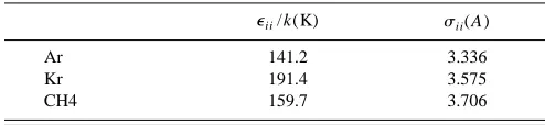
TABLE III. Lennard-Jones potential parameters for argon, krypton, and methane.
eii/k(K) sii(A)
Ar 141.2 3.336
Kr 191.4 3.575
We used the same Lennard-Jones parameters as Cottin and Monson; the diameter (sii) and well-depth (eii) for ar-gon, krypton, and methane are listed in Table III. We worked in reduced units T*5kT/e11 and P*5Ps113/e11. For P 51 atm, the corresponding reduced pressures are P*
50.001 93 ~argon!, P*50.001 75 ~krypton!, and P*
50.002 43~methane!.
The initial condition for the Gibbs–Duhem integration calculations came from the simulation data of Agrawal and Kofke37who calculated the solid–liquid equilibrium line for a single component Lennard-Jones system. They obtained a reduced melting temperature of T*50.687 for the range of reduced pressures, P*50.0008 to 0.008. In our calculations, we started with an initial condition of T1*5kT1/e11 50.687, where T1* and T1 are the reduced and absolute melting temperatures of component 1, respectively. We esti-mated the uncertainty in the simulation data by performing three Gibbs–Duhem integration simulations for each mixture and calculating the standard deviation of the temperature and mole fractions of the liquid and solid phases at each coexist-ence point. In all three mixtures, the standard deviation in coexistence temperature, kT/e11, is less than 0.2% and in mole fraction, x2, is less than 0.6%.
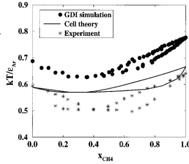
Figure 2 shows the temperature-composition phase dia-gram for the argon–methane system obtained using Gibbs– Duhem integration starting from pure methane solid–liquid coexistence, along with the cell theory prediction of Cottin and Monson and the experimental results of van’t Zelfde
et al.;46 the cell theory and experimental data have been re-duced with the Lennard-Jones parameters given in Table III. The diameter ratio issAr/sCH
450.9 and the well-depth ratio
is eAr/eCH
450.88. We obtain a minimum azeotrope similar
to the experimental data and cell theory prediction. A glance at the comparison of the ability of simulations and theory to predict experimental behavior would, at first, lead one to think that the theory is more accurate than the simulations. However, as Cottin4 points out, direct comparison of theo-retical predictions with experimental data is difficult because inadequacies in the potential model coupled with simplifying
approximations made in the theory could lead to error can-cellation. This cancellation effect is illustrated in Fig. 2 where the Lennard-Jones model ~simulation! over predicts melting temperatures for real systems~experiments!, and cell theory under predicts melting temperatures for the Lennard-Jones model. There is a good agreement in the predicted azeotrope composition between cell theory and the Lennard-Jones model, although neither predicts the azeotrope compo-sition found in experiments. After making these compari-sons, it is also useful to compare the phase diagram of this Lennard-Jones mixture with a hard-sphere mixture of the same diameter ratio to determine whether attractive interac-tions are contributing to the type of phase behavior observed. In this case, a hard-sphere mixture with the diameter ratio sAr/sCH
450.9 would also display azeotrope phase behavior.
Figure 3 shows the temperature-composition phase dia-gram of the krypton–methane system obtained using Gibbs– Duhem integration starting from pure methane solid–liquid coexistence, along with the cell theory prediction and the experimental results of Veith and Schroder.47 The diameter ratio is sKr/sCH
450.96 and the well-depth ratio iseKr/eCH4
51.2. We obtain a spindle-shaped phase diagram very simi-lar to the experimental data and cell theory prediction. A hard-sphere mixture with the diameter ratio sKr/sCH
450.96
would also display solid solution phase behavior.
Figure 4 shows the temperature-composition phase dia-gram for the argon–krypton system obtained using Gibbs– Duhem integration starting from pure argon solid–liquid co-existence, along with the cell theory prediction and the experimental results of Heastie.48Here the diameter ratio is sAr/sKr50.93 and the well-depth ratio iseAr/eKr50.74. We obtain a spindle-shaped phase diagram similar to the experi-mental data and the cell theory prediction. The simulation matches the shape of the experimental data, especially in the argon-rich region where the temperature-composition line tends to level off. A hard-sphere mixture with a diameter ratiosAr/sKr50.93 would not exhibit solid solution behavior but instead would have a minimum azeotrope. This suggests
FIG. 2. Temperature vs. composition solid–liquid phase diagram for the argon–methane system at 1 atm. The filled circles represent Gibbs–Duhem integration~GDI!simulations, the solid line corresponds to the Cottin and Monson’s cell theory6prediction, and the stars correspond to van’t Zelfde
et al.46experiments.
that the intermolecular attractions between molecules can be a significant factor in determining the type of solid–liquid phase diagram observed.
B. Influence of attractions on phase behavior
As we have discussed in Sec. I, five of the six different types of solid–liquid phase diagrams for binary mixtures can be predicted by using a hard-sphere model with an appropri-ate diameter ratio. Of the three Lennard-Jones mixtures dis-cussed thus far, we have seen one instance ~argon–krypton! where the difference in attractive interactions was large enough to change the type of phase diagram observed from azeotrope~hard sphere!to solid solution~Lennard-Jones!. In order to get a better idea of what role attractive interactions play in solid–liquid mixture phase equilibria, we performed a systematic investigation of how solid–liquid phase dia-grams change as a function of both Lennard-Jones diameter ratio (s11/s22) and well-depth ratio (e11/e22).
All of the phase diagrams presented in this section were calculated at a reduced pressure, P*50.002, which corre-sponds to a real pressure of 1 atm using the Lennard-Jones parameters for argon. Due to the large number of mixtures investigated, we did not estimate error bars for the simula-tion data but we expect the uncertainty to be similar to the uncertainty estimated for the simulation data in Figs. 2–4.
To begin our investigation, we examined two limiting cases: sizes are equal (s11/s2251) while attractions are var-ied, and attractions are equal (e11/e2251) while sizes are varied. The ultimate limiting case, a binary mixture with s11/s2251 and e11/e2251, is uninteresting; the temperature-composition phase diagram would simply be a horizontal line at T*50.687 since the components are indis-tinguishable. Phase diagrams were calculated for binary mix-tures with a diameter ratios11/s2251 and well-depth ratios e11/e2250.65, 0.75, 0.85, 0.90, and 0.95. Figure 5 shows temperature-composition phase diagrams for these binary mixtures. All of the mixtures form solid solutions with a spindle shape. Ase11/e22 decreases~attractions among
spe-cies 2 particles become stronger!, the melting point tempera-ture of species 2 increases and the degree of phase separation
~width of the spindle!increases.
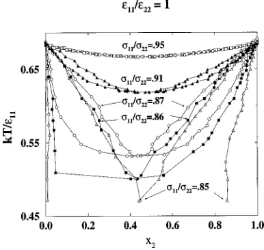
We also calculated phase diagrams for binary mixtures with a well-depth ratio e11/e2251 and diameter ratios s11/s2250.85, 0.86, 0.87, 0.88, 0.9, 0.91, 0.93, 0.94, and 0.95. Figure 6 shows selected temperature-composition phase diagrams for these binary mixtures. An azeotrope phase diagram is obtained for s11/s2250.95. As s11/s22 decreases from 0.95 to 0.86, the azeotrope temperature de-creases and the degree of phase separation on either side of the azeotrope composition increases. The azeotrope tempera-ture decreases as s11/s22 decreases because for increasing size differences, the liquid phase becomes more stable than the solid phase.49Ats11/s2250.86, the solidus line takes a steep drop in temperature over the composition range x2 50 to 0.05, and as a result, the shape of the azeotrope ap-pears distorted. At s11/s2250.85 the solidus line is no
FIG. 4. Temperature vs. composition solid–liquid phase diagram for the argon–krypton system at 1 atm. The filled circles represent Gibbs–Duhem integration~GDI!simulations, the solid line corresponds to the Cottin and Monson’s cell theory6prediction, and the stars correspond to Heastie’s48 experiments.
FIG. 5. Temperature vs. composition solid–liquid phase diagrams for Lennard-Jones binary mixtures at diameter ratio, s11/s2251.0 and well-depth ratios e11/e2250.65, 0.75, 0.85, 0.90, and 0.95. Lines are drawn through the simulation points for clarity.
longer continuous across the entire range of composition and a eutectic phase diagram is obtained. Thus, we conclude that an azeotrope to eutectic transition occurs between s11/s22 50.85 and 0.86. In comparison, Kranendonk and Frenkel19 found an azeotrope to eutectic transition for hard-sphere mixtures at s11/s2250.875.
Next, we attempted to establish boundaries for solid so-lution, azeotrope, and eutectic phase behavior ine11/e22 ver-sus s11/s22 parameter space. We calculated five series of phase diagrams at diameter ratioss11/s2250.85, 0.875, 0.9, 0.925, and 0.95. Within each s11/s22series, the well-depth ratio e11/e22was varied from 0.45 to 1.6.
In the first series~not shown!, we calculated phase dia-grams for binary mixtures with s11/s2250.95 and e11/e22 50.55, 0.65, 0.75, 1.0, 1.1, 1.2, 1.3, 1.4, and 1.6. We found solid solution phase diagrams for all the mixtures in this series, except ate11/e2251.0 where, as described above, the
phase diagram displayed a minimum azeotrope. As e11/e22 moves away from unity, the width of the spindle increases. A hard-sphere mixture with this diameter ratio has a solid so-lution phase diagram.
In the second series, we calculated phase diagrams for binary mixtures with s11/s2250.925 and e11/e2250.625, 0.8, 1.0, 1.2, 1.4, and 1.6. Figure 7 shows selected temperature-composition phase diagrams for binary mixtures from this series. An azeotrope phase diagram is obtained for e11/e2251.0. Ase11/e22decreases from 1 to 0.8, the melting point of pure component 2 increases and the azeotrope tem-perature increases. When the azeotrope temtem-perature is equal to the melting point temperature of pure component 1 (e11/e2250.625), the azeotrope disappears and the phase diagram becomes a solid solution. Conversely, as e11/e22 increases from 1 to 1.2, the melting point temperature of pure component 2 decreases and the azeotrope temperature decreases. When the azeotrope is equal to the melting point of pure component 2 (e11/e22.1.2), the azeotrope disap-pears and the phase diagram becomes a solid solution. As e11/e22 increases from 1.2 to 1.6, the melting point of spe-cies 2 decreases and the degree of phase separation increases. A hard-sphere mixture with this diameter ratio has an azeo-trope phase diagram.
In the third series, we calculated phase diagrams for bi-nary mixtures with s11/s2250.9 and e11/e2250.45, 0.65, 0.85, 0.9, 1.0, 1.05, 1.1, 1.2, 1.4, and 1.6. Figure 8 shows selected temperature-composition phase diagrams for binary mixtures from this series. An azeotrope phase diagram is obtained for e11/e2251.0. As e11/e22 decreases from 1 to 0.65, the melting point of pure component 2 increases and the azeotrope temperature increases. As e11/e22 decreases from 0.65 to 0.45, the azeotrope disappears and the phase diagram becomes a simple peritectic. A simple peritectic phase diagram is characterized by a peritectic temperature at which the liquid composition is either greater than or less than the compositions of the two solid phases with which it coexists. The inset in Fig. 8 shows the region of the peritectic
FIG. 7. Temperature vs. composition solid–liquid phase diagrams for Lennard-Jones binary mixtures at diameter ratio,s11/s2250.925 and well-depth ratiose11/e2250.625, 0.8, 1.0, 1.2, and 1.6.
FIG. 8. Temperature vs. composition solid–liquid phase diagrams for Lennard-Jones binary mixtures at diameter ratio, s11/s2250.9 and well-depth ratios e11/e2250.45, 0.65, 1.0, 1.4, and 1.6. The inset shows the region around the peritectic temperature at x250 – 0.1 fore11/e2250.45.
phase diagram between the compositions, x25020.1. As e11/e22 increases from 1 to 1.4, the melting point tempera-ture of pure component 2 decreases and the azeotrope tem-perature decreases. When the azeotrope temtem-perature is equal to the melting point of pure component 2, the azeotrope dis-appears and the phase diagram becomes a solid solution. As e11/e22increases from 1.4 to 1.6, the phase diagram changes from a solid solution to a simple peritectic. A hard-sphere mixture with this diameter ratio has an azeotrope phase dia-gram.
In the fourth series, we calculated phase diagrams for binary mixtures with s11/s2250.875 and e11/e2250.625, 0.8, 1, 1.2, 1.4, and 1.6. Figure 9 shows selected temperature-composition phase diagrams for binary mixtures from this series. An azeotrope phase diagram is obtained for e11/e2251.0. As e11/e22 decreases from 1 to 0.625, the melting point of pure component 2 increases and the azeo-trope temperature increases. As e11/e22 increases from 1 to 1.2, the melting point temperature of pure component 2 de-creases and the azeotrope temperature dede-creases. Ate11/e22 51.2, the solidus line takes a steep drop in temperature over the composition range x250 to 0.1 and as a result, the shape of the azeotrope appears distorted. Ase11/e22increases from 1.2 to 1.6, the phase diagram changes from an azeotrope to a eutectic. A hard-sphere mixture with this diameter ratio shows a transition between azeotrope and eutectic phase be-havior.
In the fifth and final series, we calculated phase diagrams for binary mixtures with s11/s2250.85 and e11/e22 50.625, 0.8, 0.9, 1.0, 1.1, and 1.6. Figure 10 shows selected temperature-composition phase diagrams for binary mixtures from this series. A eutectic phase diagram is obtained for e11/e2251.0. As e11/e22 decreases from 1 to 0.625, the melting point of pure component 2 increases and the eutectic temperature increases. As e11/e22 increases from 1 to 1.6, the melting point temperature of pure component 2 decreases and the eutectic temperature decreases. A hard-sphere mix-ture with this diameter ratio has a eutectic phase diagram.
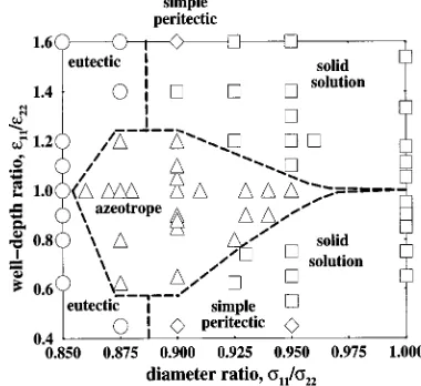
In Fig. 11, we show the regions ofs11/s22 vs.e11/e22
parameter space where the four types of solid–liquid phase diagrams ~solid solutions, azeotropes, eutectics, and simple peritectics! are found for the Lennard-Jones model. Each mixture studied in this paper is given a symbol correspond-ing to the type of phase diagram calculated via a Gibbs– Duhem integration simulation. We did not calculate phase diagrams for s11/s2251 and e11/e22.1 because due to symmetry the phase diagrams in this region will be identical to the phase diagrams for e11/e22,1.
Using these simulation results, boundaries separating the regions of solid solution, azeotrope, and eutectic phase be-havior have been estimated. Boundaries for the peritectic re-gion have not been estimated because simple peritectics oc-curred only a few times. Betweens11/s2250.95 and 1, solid solution type phase diagrams are found everywhere except for a narrow region near e11/e2251 where azeotropes are formed because the melting points of the pure components are nearly equal.25 As s11/s22 decreases below 0.95, this azeotropic region broadens and then narrows again as s11/s22 approaches 0.86, forming a fish-shaped region whose maximum height spans the rangee11/e2250.6 to 1.2. The region outside of the azeotrope region switches from solid solution to eutectic as the diameter ratio s11/s22 de-creases below 0.9.
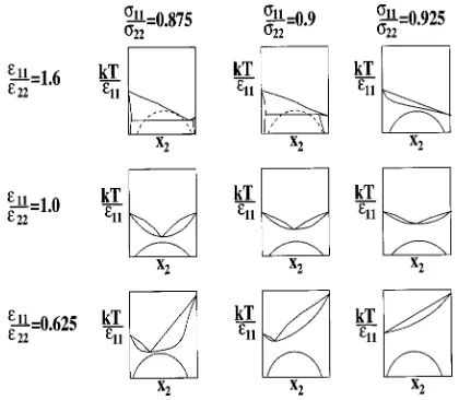
To understand how and why variations in the attractive interactions lead to the boundaries shown in thee11/e22 ver-suss11/s22parameter space displayed in Fig. 11, it is help-ful to consider the schematic phase diagrams for the selected mixtures shown in Fig. 12. The columns correspond to mix-tures with constant diameter ratios,s11/s2250.875, 0.9, and 0.925, and the rows correspond to mixtures with constant well-depth ratios, e11/e2250.625, 1.0, and 1.6. The solid– liquid lines are based on our simulation results. The solid– solid equilibrium lines are based on our best guess as to how the upper critical solution temperature of the solid–solid im-miscibility dome shifts with variations in well-depth ratio. Underpinning this guess is quasichemical theory,50,51which tells us that the upper critical solution temperature increases
FIG. 10. Temperature vs. composition solid–liquid phase diagrams for Lennard-Jones binary mixtures at diameter ratio,s11/s2250.85 and well-depth ratiose11/e2250.625, 1.0, and 1.6.
as the attractions between like molecules become stronger than the attractions between unlike molecules. This means that the upper critical solution temperature will increase as e11/e22increases above unity or decreases below unity. This is shown schematically in Fig. 12.
In the s11/s2250.925 column, the phase diagram is a solid solution at e11/e2251.6. As the well-depth ratio e11/e22 decreases, the melting point temperature of compo-nent 2 increases and the solid–liquid lines ‘‘pull away’’ from the solid–solid immiscibility dome. In thes11/s2250.9 col-umn, the phase diagram is a simple peritectic at e11/e22 51.6. As the well-depth ratio decreases, the solid–liquid lines move away from the underlying solid–solid immisci-bility dome ~shown in dashed lines! and the phase diagram becomes an azeotrope. In the s11/s2250.875 column, the phase diagram is a eutectic at e11/e2251.6. As the well-depth ratio decreases, the solid–liquid lines move away from the solid–solid immiscibility dome and the phase diagram becomes an azeotrope.
In the e11/e2251.6 row, the phase diagram is a solid solution ats11/s2250.925. As the diameter ratio decreases, the solid–liquid lines ‘‘fall’’ because the liquid phase can accommodate the larger differences in size easier than the solid phase49 and the phase diagram becomes a simple peri-tectic at s11/s2250.9 and a eutectic ats11/s2250.875. In the e11/e2251.0 row, the phase diagram is an azeotrope at s11/s2250.925. As the diameter ratio decreases and the solid–liquid lines fall, the azeotrope temperature decreases. In the e11/e2250.625 row, the phase diagram is a solid so-lution at s11/s2250.925. As the diameter ratio decreases and the solid–liquid lines fall, the phase diagram becomes an azeotrope.
IV. SUMMARY
The Gibbs–Duhem integration technique was combined with semigrand canonical Monte Carlo simulations to calcu-late solid–liquid phase diagrams for binary Lennard-Jones mixtures.
We calculated phase diagrams for model mixtures: argon–methane, argon–krypton, and krypton–methane, and compared them to cell theory predictions and experimental data. We found that cell theory qualitatively predicts the shape of phase diagrams for Lennard-Jones mixtures. Com-parison of our simulation results for the argon–krypton Lennard-Jones system with hard-sphere results at the same diameter ratio (sAr/sKr50.93) indicated that the presence of attractive interactions can change the type of phase diagram observed from azeotrope ~hard-sphere! to solid solution
~Lennard-Jones!. This suggested that we further explore the effect of asymmetry in the attractions on the types of phase diagrams observed.
We simulated 56 binary Lennard-Jones mixtures over a range of diameter ratios s11/s2250.85– 1.0 and well-depth ratios e11/e2250.45– 1.6. We found that for well-depth ra-tios of unity~equal attractions among species!, phase behav-ior indicative of azeotropes and eutectics is observed for di-ameter ratios ranging from 0.85 to 1. Much to our surprise, we also found that varying the attractive interactions at a fixed diameter ratio can perturb the type of solid–liquid phase diagram obtained, a trend that previously6,8 had not been explored in Lennard-Jones mixtures.
There are several areas for further study. First, it would be helpful to know where the solid–solid immiscible dome is located relative to the solid–liquid lines that we have calcu-lated in this paper. Determining solid–solid equilibrium lines would give a more complete picture of how the solid–liquid and solid–solid equilibrium lines merge as we vary param-eters and observe transitions between solid solutions, azeo-tropes, eutectics, and simple peritectics. Second, it would be interesting to repeat this type of investigation for s11/s22 ,0.85, a region where several ordered solid phases are known to be stable.
1M. Matsuoka, Bunri Gijutsu 7, 245~1977!.
2X. Cottin and P. A. Monson, J. Chem. Phys. 99, 8914~1993!. 3
X. Cottin and P. A. Monson, J. Chem. Phys. 102, 3354~1995!. 4X. Cottin, Ph.D. thesis, University of Massachusetts, 1996.
5X. Cottin, E. P. A. Paras, C. Vega, and P. A. Monson, Fluid Phase
Equi-libria 117, 114~1996!. 6
X. Cottin and P. A. Monson, J. Chem. Phys. 105, 10022~1996!. 7
D. W. Oxtoby, Nature~London!347, 725~1990!.
8S. W. Rick and A. D. J. Haymet, J. Chem. Phys. 90, 1188~1989!. 9S. W. Rick and A. D. J. Haymet, J. Phys. Chem. 94, 5212~1990!. 10X. C. Zeng and D. W. Oxtoby, J. Chem. Phys. 93, 4357~1990!. 11
A. R. Denton and N. W. Ashcroft, Phys. Rev. A 42, 7312~1990!. 12D. Frenkel and B. Smit, Understanding Molecular Simulations ~
Aca-demic, San Diego, 1996!.
13D. Frenkel and A. J. C. Ladd, J. Chem. Phys. 81, 3188~1984!. 14
R. L. Rowley, Statistical Mechanics for Thermophysical Property
Calcu-lations~Prentice Hall, Engelwood Cliffs, New Jersey, 1994!.
15M. D. Eldridge, P. A. Madden, and D. Frenkel, Nature~London!365, 35 ~1993!.
16M. D. Eldridge, P. A. Madden, and D. Frenkel, Mol. Phys. 79, 105~1993!. 17
M. D. Eldridge, P. A. Madden, and D. Frenkel, Mol. Phys. 80, 987~1993!. 18W. G. T. Kranendonk and D. Frenkel, Mol. Phys. 72, 699~1991!. 19W. G. T. Kranendonk and D. Frenkel, Mol. Phys. 72, 679~1991!. FIG. 12. Schematic phase diagrams showing how variations in diameter
20D. A. Kofke, Mol. Simul. 7, 285~1991!.
21D. A. Kofke and E. D. Glandt, J. Chem. Phys. 87, 4881~1987!. 22D. A. Kofke and E. D. Glandt, Mol. Phys. 64, 1105~1988!. 23
W. G. Hoover and F. H. Ree, J. Chem. Phys. 49, 3609~1968!. 24M. J. Vlot, J. C. van Miltenburg, H. A. J. Oonk, and J. P. van der Eerden,
J. Chem. Phys. 107, 10102~1997!.
25J. S. Rowlinson, Liquids and Liquid Mixtures ~Butterworth Scientific,
London, 1982!. 26
M. J. Vlot and J. P. van der Eerden, J. Chem. Phys. 106, 2771~1997!. 27K. S. Shing and K. E. Gubbins, Mol. Phys. 46, 1109~1982!.
28M. J. Vlot, S. Claassen, H. E. A. Huitema, and J. P. van der Eerden, Mol.
Phys. 91, 19~1997!. 29
B. Widom, J. Chem. Phys. 39, 2808~1963!. 30
J. M. Prausnitz, R. N. Lichtenthaler, and E. G. de Azevedo, Molecular
Thermodynamics of Fluid-Phase Equilibria, 2nd ed.~Prentice Hall, Engle-wood Cliffs, New Jersey, 1986!.
31A. Z. Panagiotopoulos, Mol. Phys. 61, 813~1987!. 32
A. Z. Panagiotopoulos, N. Quirke, M. Stapleton, and D. J. Tildesley, Mol. Phys. 63, 527~1988!.
33A. Z. Panagiotopoulos, Mol. Simul. 9, 1~1992!. 34D. A. Kofke, Mol. Phys. 78, 1331~1993!. 35
D. A. Kofke, J. Chem. Phys. 98, 4149~1993!. 36
R. Agrawal, M. Mehta, and D. A. Kofke, Int. J. Thermophys. 15, 1073 ~1994!.
37R. Agrawal and D. A. Kofke, Mol. Phys. 85, 43~1995!.
38M. H. J. Hagen E. J. Meijer, G. C. A. M. Mooij, D. Frenkel, and H. N. W.
Lekkerkerker, Nature~London!365, 425~1993!.
39E. J. Meijer and D. Frenkel, J. Chem. Phys. 100, 6873~1994!. 40
F. W. Tavares and S. I. Sandler, AIChE. J. 43, 218~1997!. 41
D. A. Kofke, in Monte Carlo Methods in Chemistry, edited by D. M. Ferguson, J. I. Siepmann, and D. G. Truhlar ~Interscience, New York, 1998!, Vol. 105, Chap. 13, p. 405.
42M. Mehta and D. A. Kofke, Chem. Eng. Sci. 49, 2633~1994!.
43B. Carnahan, H. A. Luther, and J. O. Wilkes, Applied Numerical Methods ~Wiley, New York, 1969!.
44M. P. Allen and D. J. Tildesley, Computer Simulation of Liquids~
Claren-don, Oxford, 1987!. 45
J.-P. Hansen and L. Verlet, Phys. Rev. 184, 151~1969!.
46P. van’t Zelfde, M. H. Omar, H. G. M. le Pair-Schroten, and Z. Dokoupil,
Physica~Amsterdam!38, 241~1968!.
47H. Veith and E. Schroder, Z. Phys. Chem. Abt. A 179, 16~1937!.
48R. Heastie, Nature~London!176, 747~1955!. 49
W. Hume-Rothery, R. E. Smallman, and C. W. Haworth, The Structure of
Metals and Alloys~The Metals and Metallurgy Trust, London, 1969!. 50A. Prince, Alloy Phase Equilibria~Elsevier, Amsterdam, 1966!.
51P. Gordon, Principles of Phase Diagrams in Materials Systems~Krieger,