ABSTRACT
SUN, HANG. Sourcing Risk Detection and Prediction with Online Public Data: An
Application of Machine Learning Techniques in Supply Chain Risk Management. (Under the direction of Dr. Robert Handfield).
The classic methods of studying supply chain risks are based on survey analysis and historical records analysis. Developments in information science and the expansion of supply chain globalization now require analytical methods to be more efficient in providing an objective view on risk management. In this dissertation, a semi-automatic process was
designed to detect and assess the upstream supply chain risks in apparel production industries in ten countries. This process includes online data collection, information extraction,
evaluation digitalization and risk distribution visualization. A web crawler based on keywords was created to collect external data, consisting primarily of public information available online, for risk analysis. For information extraction and digitalization, a modified version of the Analysis of Competing Hypotheses method was used to gather opinions about each risk factor in each country from available data, and to generate two assessments for each risk factor: (1) likelihood score and (2) supply chain impact score. To reduce labor and time costs, this dissertation applies machine learning techniques in the analysis process. It
Sourcing Risk Detection and Prediction with Online Public Data: An Application of Machine Learning Techniques in Supply Chain Risk Management
by Hang Sun
A dissertation submitted to the Graduate Faculty of North Carolina State University
in partial fulfillment of the requirements for the degree of
Doctor of Philosophy
Operations Research
Raleigh, North Carolina 2019
APPROVED BY:
_______________________________ _______________________________ Dr. Robert Handfield Dr. Hans S. Heese
Committee Chair
ii DEDICATION
iii BIOGRAPHY
iv ACKNOWLEDGMENTS
I would like to thank my advisor, Dr. Robert Handfield. His consistent guidance, advice and support led me to accomplish much throughout this journey. His encouragement and patience helped me through the most difficult time of my study. The work ethic I’ve learned from him will benefit me further after graduation. My sincere thanks also go to my committee
members, Dr. Hans Sebastian Heese, Dr. Bill Rand, Dr. Lori Rothenberg, and my external consultant, Dr. Arun Gupta, for their invaluable teachings and mentorship. Their assistance and insightful comments on my research guided me to work toward a better dissertation. I’ve been fortunate to be a student of this committee.
I am grateful to Troy Pinkins and the many assistants from SCRC I’ve worked with. I’ve been lucky to work with and learn from these excellent people on various projects. I’d like to give special thanks to Shaunak Sathe, Lijun Zhou, Simone Handfield, Namratha Prabhu, Arvind S. Prabakar, Yash M. Shah, Sumedh S. Hegde, Anurag Singal, and Stitha Panda for their hard work on data collection and peer review, which is the foundation of my dissertation research. I also want to thank Kelei Gong, who helped a lot in my coding problems.
Finally, I want to thank my mother, Hongying Li, and grandmother, Guilian Cai, for their endless love, support and encouragement. They are the resources of my inner strength. The last but not least, I’m grateful to my dear friends Jia Hou and Xiao Qiu for their
v
TABLE OF CONTENTS
LIST OF TABLES ... vii
LIST OF FIGURES ... viii
Chapter 1: Problem Introduction ...1
1.1 Research Questions ...3
1.2 General Application Assumptions ...5
1.3 Dissertation Structure ...7
Chapter 2: Literature Review ...8
2.1 Global Sourcing Risk Management ...8
2.2 Machine Learning and Data Analytics in Supply Chain Risk Management ...10
2.3 Analysis of Competing Hypotheses ...13
2.4 Machine Learning Basics ...15
2.4.1 Supervised Learning ...16
2.4.2 Training Data, Validation Data and Test Data ...18
2.4.3 Support Vector Machine (SVM) ...19
2.4.4 Naïve Bayes Classifier ...26
Chapter 3: Methodology ...32
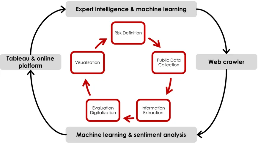
3.1 Process Flowchart ...33
3.2 Risk Definition and Hypotheses ...35
3.3 Data Collection and Management ...44
3.3.1 Online Data Collection ...44
3.3.2 Database Design and Management ...46
3.4 Risk Quantification ...48
3.4.1 Extended ACH ...48
3.4.2 Risk Assessment ...54
3.5 Machine Learning Application ...58
3.5.1 Data Cleaning ...59
3.5.2 Sentence Extraction ...62
3.5.3 Feature Extraction ...65
3.5.4 Feature Selection ...69
3.5.5 SVM Models ...72
3.5.6 Naïve Bayes Classifier ...73
3.5.7 Model Evaluation ...74
Chapter 4: Result Presentation ...84
4.1 Data Description ...84
4.1.1 Overall Data ...84
4.1.2 Country Specific Data ...86
4.2 Visualization of Risks ...91
4.2.1 Risk Distribution ...94
4.2.2 Attention-Worthy Risks ...98
4.2.3 Risk Shift over Time ...102
4.3 Risk Measurement Validation ...109
4.3.1 Raw Data Description ...109
4.3.2 Risk Assessment Transformation ...111
vi
4.3.4 Regression Analysis ...121
4.3.5 Summary and Discussion ...129
4.4 Text Classification Performance ...132
4.4.1 Imbalanced Data ...135
4.4.2 Bias and Variance ...137
4.4.3 Validation Curves ...139
4.4.4 Model Selection ...144
4.4.5 Interesting Features ...145
4.4.6 Adjusted Application ...147
Chapter 5: Summary and Discussion ...155
5.1 Supply Chain Risk Assessment ...155
5.2 Machine Learning Application ...157
References ...159
vii LIST OF TABLES
Table 2.1 Types of Machine Learning ...16
Table 3.1 Risk Definitions and Categories ...38
Table 3.2 Sample Hypotheses ...43
Table 3.3 Summary for Manual Data Collection ...45
Table 3.4 Credibility and Relevance ...50
Table 3.5 Risk Ratings in Extended ACH ...51
Table 3.6 Analysis Summary -- Count of Words and Sentences ...60
Table 3.7 Examples of Counting Vectorizer ...67
Table 4.1 Manual Risk Assessment Matrix: Supply Chain Impact Scores ...92
Table 4.2 Manual Risk Assessment Matrix: Likelihood of Occurrence Scores ...93
Table 4.3 Samples from Fail Records ...110
Table 4.4 Weights of Dissertation Risk Factors in CompanyA Risks ...113
Table 4.5 CompanyA Risk Assessment Matrix: Supply Chain Impact Scores ...115
Table 4.6 CompanyA Risk Assessment Matrix: Likelihood of Occurrence Scores ...116
Table 4.7 CompanyA Risk Basic Internal Matrix: Fail Severity ...118
Table 4.8 CompanyA Risk Basic Internal Matrix: Count of Fails ...119
Table 4.9 Supply Chain Impact Score and Fail Severity: Linear Regression Models ...123
Table 4.10 Supply Chain Impact Score and Fail Severity: Quadratic Regression Models .126 Table 4.11 Model Selection Results ...129
Table 4.12 F1 Scores ...145
viii LIST OF FIGURES
Figure 2.1 Supervised Learning ...17
Figure 2.2 Support Vector Machine (SVM) ...20
Figure 2.3 Samples of Nonlinearly Separable Data ...22
Figure 2.4 Parameter C Controlling the Margin of Margin ...23
Figure 2.5 Hyperplane in Higher Dimension Space ...23
Figure 3.1 Framework of External Risk Analysis ...33
Figure 3.2 Design of Web Crawler ...46
Figure 3.3 IDEF1X Model of Database ...47
Figure 3.4 Original ACH Method ...49
Figure 3.5 The Flowchart of Data Cleaning ...61
Figure 3.6 The Flowchart of Sentence Extraction ...64
Figure 3.7 Examples of Univariate Statistical Test ...71
Figure 3.8 Confusion Matrix for a Binary Classification ...75
Figure 3.9 Learning Curves for Bias and Variance ...82
Figure 4.1 Overall Article Distribution ...85
Figure 4.2 Article Distribution in Countries ...87
Figure 4.3 Risk Distribution over Country ...95
Figure 4.4 Attention-Worthy Risks ...99
Figure 4.5 Risk Shift over Time ...103
Figure 4.6 Application of Machine Learning Classifier ...134
Figure 4.7 Imbalanced Data ...136
ix
Figure 4.9 Validation Curves: Parameter ...140
Figure 4.10 Validation Curves -- NB: Sentence Range ...143
Figure 4.11 Validation Curves -- SVM: Sentence Range ...143
Figure 4.12 Top 50 Features ...146
Figure 4.13 Imbalanced Global Data ...148
Figure 4.14 Learning Curves for Global Data ...149
Figure 4.15 Validation Curves for Global Data: Parameter ...150
Figure 4.16 Validation Curves for Global Data: Sentence Range ...151
1 CHAPTER 1
Problem Introduction
From 2014 to 2017, Brazils went through a long, difficult time, with severe drought in the
southeast, including areas around Sao Paulo and Rio de Janeiro, the country’s most prosperous cities. The drought in Sao Paulo has been described as the worst in 100 years (Baine, 2014). Since 70% of Brazil’s electricity is generated by hydropower, the drought led
directly to a decrease of around 80% in hydroelectric power (Leahy, 2015). Lack of both electricity and water caused a reduction in production capacity in those cities. To maintain
both production and citizens’ normal life, more expensive alternative power using oil-based and carbon-based fuels were used. The increased cost resulted in increased water and electricity prices.
However, the drought didn’t arrive without warning. In fact, as early as 2013, the website BBC Brasil expressed concern about energy shortages caused by the drought
(Barrucho, 2013). According to this report, drought continued to be a hazard is Brazil until 2017.
Since the late 1990s, Nike, the world's largest supplier of athletic shoes and apparel
and a major manufacturer of sports equipment, has faced large public protests after being accused of using sweatshops in developing countries to pursue a high profit. According to
2 sustainability strategy, “Nike is still on the cusp of public review and judgement” (Schifrin,
et al., 2013). Whenever new scandals arise about human rights in factories in developing countries, Nike will face public scrutiny and accusation.
Both the Brazil drought and the Nike human rights cases were brought to worldwide
attention by widespread access to public information and media opinion. As the digital age expands, a rapidly increasing amount of information is becoming accessible to the public.
This poses a question: can businesses take advantage of the availability of public information?
Public information includes the opinions of people with various backgrounds. Thus,
compared with internal data from a company’s “private” database, the external public data is more objective. Internal data usually refers to audit data, historical records, survey responses,
etc., while external public data could be in various formats including videos, text, pictures, etc. which could contain some hidden information. In addition, external public data is much cheaper and easier to obtain than internal data.
On the other hand, there are cons about external public data. The objective value of public data depends upon the various backgrounds of both the data and the data’s authors.
Most of the information is not accurate enough for a deep study of a certain topic. Therefore, instead of contributing valuable information, most external data only adds noise to the database.
What’s more, the unlimited kind of data formats in which external data is presented makes the data unstructured. If we would like to study the supply chain of a product line
3 materials, its cost, etc. There also might be thousands of people posting information and
opinions on social media talking the design, price, or the function of Air Max shoes. The latter category may contain a short message, an emoji, a photo, or a video. This massive unstructured data set makes extracting the information desired very challenging.
This dissertation proposes a semi-automatic assessment process to explore using external data. It is designed to evaluate certain types of supply chain risks by studying public
online news.
1.1 Research Questions
This dissertation focuses on three questions:
• When does the risk appear in the supply chain? And how will it impact the supply
chain?
• How may we assess the appearance and severity of a risk with external public
data?
• How may we apply the machine learning techniques in this assessment?
To answer the first question, we define the supply chain risk first. “Supply chain risk is the potential loss for a supply chain in terms of its target values of efficiency and
effectiveness evoked by uncertain developments of supply chain characteristics whose changes were caused by the occurrence of triggering events.” (I. Heckmann, T. Comes, & S.
4 potential meaningful influence on the supply chain. The occurrence could be assessed by its
probability, while the event’s influence is usually described as its “vulnerability or resilience” (I. Heckmann, et al., 2015).
To assess the supply chain risk, one must model the trigger events as potential levels
of impact on the supply chain (I. Heckmann, et al., 2015), for example, disturbance (Svensson, 2002), disruption (Sheffi & Rice Jr, 2005), and disaster (I. Heckmann, et al.,
2015). This dissertation adopts this concept of risk definition. We will use two
measurements, likelihood of happening and supply chain impact, to assess a risk factor. However, some adjustments have been made to make the concepts applicable in the study.
Definitions will be detailed in Chapter 3.
The second question is an extension of the first one. We will devise some theoretical
definitions to answer the first question. For the second one, we will conduct actual analysis. The parameters of the real problem are stated in section 1.2. The detailed designs and analytical method are described in Chapter 3.
The third question requires a more efficient tool compared with the solution to question two. Since we’re dealing with massive, unstructured data, it is quite expensive for
the researchers to do the assessments manually. This point will be better explained in Chapter 3, where the detailed analytical method is introduced. To solve the problem of labor problem, some analytical technologies are applied in the study. By using data mining and machine
learning techniques, the assessments could be done automatically under supervision. The analytical techniques make it possible to repeat the assessment process periodically over
5 1.2 General Application Assumptions
Apparel & Footwear Industry
The apparel and footwear industry is the target industry of this research. The initial concept
of this project comes from a cooperative global apparel and footwear company which was seeking methods to improve its supplier audit. Due to the complexity of the apparel and
footwear industries, differences between the apparel industry and the footwear industry is not considered in this dissertation. This assumption limits the related keywords to a specific industry. Due to the overlaps among the apparel, footwear, and textile industries, including
fast fashion and so on, analysis in this dissertation is based on the data which does not completely exclude the information about related industries.
Global Outsourcing
This dissertation studies global outsourcing. Economic development and the growth of globalization have made global sourcing an attractive strategy for many companies across
industries. Outsourcing, which provides those companies with higher margins and more effective productivity, is still a trend in production industries. For those companies who are
doing business and competing globally, global sourcing is an important research topic in strategy making (Das & Handfield, 1997).
Countries
Based on materials from CompanyA, further explained in Chapter 3, 20 top countries of interest were selected for analysis. They are listed in Appendix A. Due to the amount and
6 dissertation will present only data related to these 10 countries: Argentina, Bangladesh,
Brazil, Cambodia, India, Indonesia, Mexico, Philippines, Thailand, Vietnam. Data Type
To simplify the analysis and test for the proposed process, this dissertation mainly studies
online public articles written in English. The articles include news, government reports, academic papers, etc.
External Risks in Upstream Supply Chain
Generally, supply chain risks are classified into two types: internal risks and external risks (M. Christopher, Mena, Khan, & Yurt, 2011; Goh, Lim, & Meng, 2007). The internal risks,
e.g. process risk and control risk, are mostly caused by the capabilities of the supply chain, or the sourcing strategies and management decisions made by managers. The external risks
come from outside the supply chain. For example, the demand variability caused by the market, the cost increase impacted by the resources, and the reputation damage caused by the social responsibility, could all be categorized as external risks. Due to the external nature of
public news, this dissertation considers only external risks.
In this dissertation, only the upstream supply chain is under consideration. This
project scope was generated by CompanyA’s concerns about their suppliers. Short-Term Study
The outputs of the assessment process are short-term results: even though we are looking at
supply chain information from a relative macro view, the timeliness of news provides limited information for long-term analysis. One to two years should be a reasonable time length for
7 1.3 Dissertation Structure
Chapter 1 briefly introduces the research questions in this dissertation, along with related background, and proposes some general assumptions which define the scope of the dissertation.
Chapter 2 is a literature review, which introduces related literature and states the potential contribution of the research. It also introduces basic knowledge about applied
analytical methodologies, and the improved ACH method, which enables the quantification of the text information.
Chapter 3 explains the detailed assessment process and analytical methodologies. It
explains the functions and models in each module.
Chapter 4 presents detailed analytical results, predicts risk likelihood and severity,
and states the measurement validation and machine learning model performance analysis. Chapter 5 concludes and discusses research results.
8 CHAPTER 2
Literature Review
2.1 Global Sourcing Risk Management
As the supply chain becomes more global and complex, global sourcing provides companies lower cost, more efficient production and more profits. However, numerous risks arise in
supply chain networks, such as natural disasters, unsteady political situation, labor rights activities, customs regulations, local economic recessions, etc. (C. S. Tang, 2006a). These
events make global supply chains more vulnerable to unanticipated disruptions and
corresponding consequences (Craighead, Blackhurst, Rungtusanatham, & Handfield, 2007; Fahimnia, Tang, Davarzani, & Sarkis, 2015). Global supply chain networks have multiple
tiers and numerous suppliers, subcontractors and intermedia customers; therefore, a slight glitch or disturbance among the complicated supply chain network may cause serious loss for
the purchasing companies (Markides & Berg, 1988). According to Cardoso, Barbosa-Povoa, Relvas, and Novais (2015), unanticipated disruptions in supply chains might cause serious impact on the supply chain, including production shutdowns and yield of capacity. Hendricks
and Singhal (2003) proved that glitches in the supply chain might have a significant negative impact on stock performance, even in the long term (Hendricks & Singhal, 2005; C. S. Tang,
9 As stated in Chapter 1, this dissertation mainly focuses on external risks, which
usually could not be prevented, but could be mitigated by risk management. Management of agility (H. L. Lee, 2004), flexibility (C. Tang & Tomlin, 2008), and resilience (Sheffi & Rice Jr, 2005) are three common strategies for mitigating supply chain risks (Fahimnia, et al.,
2015). While sourcing risks has been an increasing concern for many companies (Sheffi & Rice Jr, 2005; Sodhi, Son, & Tang, 2012), few have effective actions in process for risk
management (Muthukrishnan & Shulman, 2006), which makes supply chain management an attractive area for both academic researchers and supply chain executives. A framework to conduct the risk management includes identifying, assessing, mitigating, and responding to
risks (Fahimnia, et al., 2015).
The fundamental difficulty of supply chain risk management is clearly defining it
(Sodhi, et al., 2012). The definitions and interpretations of SCRM differ among researchers (Fahimnia, et al., 2015). In this dissertation, since we only consider external risks in the upstream supply chain, we adopt the concept of SCRM from Iris Heckmann, Tina Comes,
and Stefan Nickel (2015), who considered supply chain risks as a pure event-oriented concept with two attributes: the probability of occurrence and the related consequences.
Based on this concept, this dissertation develops more applicable definitions for risks, which enable text analysis and machine learning techniques to be applicable in risk management.
As in the study of Fahimnia, et al. (2015), fuzzy modeling for strategic
decision-making is the top research area in SCRM. Other mainstreams in risk management included information sharing/lean supply chain, risk theories/conceptual risk mitigation strategies,
10 However, though quantitative, analytical and formal modeling in SCRM has grown rapidly
since 2001 (Fahimnia, et al., 2015), quantification and modeling of supply chain risks is still a challenge in SCRM (Ghadge, Dani, & Kalawsky, 2012; Iris Heckmann, et al., 2015). Supply chain risk assessment is tactical in SCRM (Martin Christopher & Peck, 2004), and a
clear and adequate quantitative method is needed to guide executives to monitor the useful information, then make mitigation decisions. This dissertation is such an application of
analytical technologies in SCRM, and will be a useful supplement to the literature of risk monitoring and assessment.
2.2 Machine Learning and Data Analytics in Supply Chain Risk Management
Supply chain management researchers have developed processes to apply data science to studying supply chain activities. Bao and Datta (2014) used the unsupervised LAD model in
analyzing 10-k forms to simultaneously discover and quantify risks. Based on their methods, Westerburg and Bode (2017) analyzed annual reports to disclose supply chain risks. B. Chae
(2015) suggested a mechanism for tweets analysis on supply-chain-related topics. They developed an understanding of the prospective role of Twitter in future supply chain
management research. Gunasekaran, et al. (2017) conducted predictive analysis on extensive
survey data to investigate supply chain and organization performance. Wichmann, Brintrup, Baker, Woodall, and McFarlane (2018) used natural language processing techniques to
11 The blowout growth of machine learning applications and data analysis in supply
chain management implies the rapid change in analytical techniques in supply chain management. One sign is the change in choices of data resources. Compared with the traditional structure of data, the choices of data tend to be more various. Instead of being
limited to industrial data resources, as mentioned above, more authors have chosen secondary data as information resources. Unstructured data, and semi-structured data, including text,
figures, videos, voice, etc., could be potential information resources (Wichmann, et al., 2018). Besides, the size of data tends to increase. Large scale data structures and massive data are being used more in supply chain management. Big data is still an increasing trend in
supply chain management (Addo-Tenkorang & Helo, 2016; Hazen, Skipper, Ezell, & Boone, 2016; Wang, Gunasekaran, Ngai, & Papadopoulos, 2016; Zhong, Newman, Huang, & Lan,
2016). The speed of data update also has been a continuous concern for data analysts B. Chae (2015).
To access information most relevant to external sourcing risks, this dissertation
proposes to choose online public text articles as its main data resources. These articles include news, academic articles, government reports, etc. There are several advantages of
using public online information. The articles contain meaningful information (Bongsug Chae & Park, 2018). Academic papers (T. H. Lee, 2017; Taneja, Taneja, & Gupta, 2011),
corporate reports (Unerman, 2000), newspapers (S. Y. Lee & Carroll, 2011; L. Tang, 2012),
social media posts (B. Chae, 2015), company website pages (Chaudhri & Wang, 2007; Perry & Bodkin, 2000), and many other information sources are increasingly available in digital
12 expertise. The current research will still use text articles, but will employ advanced tools to
deal with the “noise” caused by the information explosion. Another advantage of online text data is timely, easy access to the information (Wichmann, et al., 2018). Compared with the costly and long cycle collection of industrial internal data, articles on websites can easily be
obtained through search engines. Most of the articles remain available online for a short time. Once an article is uploaded to the Internet, it can be indexed and obtained by the search
engines in time, which enables timely updates and analysis of the database.
With the unstructured text data, some classic analysis methods are no longer
applicable. Machine learning is a powerful tool for dealing with massive data. The concepts
of machine learning and data analysis overlap a great deal. This research blurs the difference between the two and regards them as the same set of analytical algorithms. In the works
listed in the first paragraph, machine learning has been proven to perform well in supply chain management. While companies have realized the importance of data-driven decisions, it is still challenging for many companies to extract, store and analyze a large volume of
complex data (Arunachalam, Kumar, & Kawalek, 2018; Sanders, 2016). Continuous development in digitalized data and sophisticated analytical technologies in supply chain
management has taken us to the era of the digitized supply chain (Rob Handfield, 2017). Machine learning is such a promising tool for realizing inexpensive information integration, value extraction, and decision making.
13 2.3 Analysis of Competing Hypotheses
Although we adopted the ACH structure in our research, we did not conduct ACH analysis. This section includes a necessary but brief introduction of ACH.
Richards (Dick) J. Heuer (2007) defined ACH thus: “Analysis of competing hypotheses, sometimes abbreviated ACH, is a tool to aid judgment on important issues
requiring careful weighing of alternative explanations or conclusions. It helps an analyst overcome, or at least minimize, some of the cognitive limitations that make prescient intelligence analysis so difficult to achieve.” It is a tool to assist analysts to think critically
and avoid bias, a process that helps them avoid common analytic pitfalls. According to Valtorta, Dang, Goradia, Huang, and Huhns (2005), “… ACH is particularly appropriate for
controversial issues when analysts want to leave an audit trail to show what they considered and how they arrived at their judgment or assessments….” As a structured analysis method, ACH is listed by the CIA as a technique to improve intelligence analysis (Primer, 2009). We
cite the eight-step procedure of ACH from Structured Analytic Techniques for Improving
Intelligence Analysis (Primer, 2009; Richards (Dick) J. Heuer, 2007):
Step 1: Identify the possible hypotheses to be considered. Use a group of analysts
with different perspectives to brainstorm the possibilities.
Step 2: Make a list of significant evidence and arguments for and against each
hypothesis.
Step 3: Prepare a matrix with hypotheses across the top and evidence down the side.
14
Step 4: Refine the matrix. Reconsider the hypotheses and delete evidence and
arguments that have no diagnostic value.
Step 5: Draw tentative conclusions about the relative likelihood of each hypothesis.
Proceed by trying to disprove hypotheses rather than prove them.
Step 6: Analyze how sensitive your conclusion is to a few critical items of evidence.
Consider the consequences for your analysis if that evidence were wrong, misleading, or
subject to a different interpretation.
Step 7: Report conclusions. Discuss the relative likelihood of all the hypotheses, not
just the most likely one.
Step 8: Identify milestones for future observation that may indicate events are taking
a different course than expected.
ACH is an easy-to-follow and reasonable decision-making tool. Instead of using it for critical thinking, we use the process of ACH to conduct supply chain risk assessments. The process of using evidence to prove or disprove the hypothesis was adjusted and is used to
extract meaningful information in evaluating supply chain risks. The process of
“diagnosticity” in ACH was extended and is used to classify text content and quantify the
15 2.4 Machine Learning Basics
Machine learning is an applicable technology based on multiple subjects, including
mathematics, statistics, and computer science. Common tasks for machine learning include
pattern recognition, diagnosis, robot control, prediction, etc. (Nilsson, 1996), and has been widely applied in many disciplines. “Any field that needs to interpret and act on data can
benefit from machine learning techniques” (Harrington, 2012). The goal of machine learning is to imitate human intelligence to study training data then solve the given problems. When we use computers to solve a problem without machine learning, we need to write an
algorithm program. This algorithm is proposed by the programmers based on previous research. In cases where specific algorithms have not been defined, or the solutions to the
problems could not be explained, we can program the computers to learn from training data or experience directly and give a solution which optimizes the performance criterion
(Alpaydin, 2014). This dissertation, for example, uses machine learning to evaluate supply
chain risks based on text information. Rating risks based on text data is not a difficult task for supply chain experts. But it is difficult for them to explain how they process the text
information in their brains. Because in natural language, the authors use various expressions to express the same opinions. They have many non-duplicate combinations of sentence structures and choices of words or phrases. Thus, it is difficult to program a specific
algorithm to command computers to do the task; machine learning is thus the appropriate technology.
16 2.4.1 Supervised Learning
In common knowledge, there are three main learning types in machine learning: supervised, unsupervised, and reinforcement learning (Raschka, 2015). We summarize the three types in Table 2.1 below:
Table 2.1 Types of Machine Learning
Type Task (Raschka, 2015) Data Method
Supervised Making predictions about unseen or future data
labeled training
data
classification, regression, etc.
Unsupervised Discovering hidden structures or patterns in data
unlabeled data clustering, principal
component, etc.
Reinforcement Improving performance based on interactions with environment
experience and
reward function
Markov decision process,
dynamic programming, etc.
This section focuses on supervised learning. The task is classification. The content below is mainly based on Python Machine Learning (Raschka, 2015), Introduction to
Machine Learning (Alpaydin, 2014) and Machine Learning in Action (Harrington,
2012). Other references will be cited throughout.
What distinguishes supervised learning from other types is the labels in the input data.
The labels are in various formats. For example, in classification problems, the labels are the nominal signs of categories; in regression problems, the labels could be continuous values. No matter what its format, the label represents the output we desire to see. In other words, we
17 variable, and the label contains the corresponding output value. We modified the figures
from Python Machine Learning (Raschka, 2015), and present the general supervised learning process in Figure 2.1.
Figure 2.1 Supervised Learning
The commonly used supervised learning algorithms include K-Nearest Neighbors,
Naïve Bayes, Support Vector Machines, Decision Trees, etc. This dissertation applies Support Vector Machine (SVM) and Naïve Bayes (NB) in the classification study. These
18 2.4.2 Training Data, Validation Data and Test Data
Figure 2.1shows that the input data set is divided into three parts: training data set, validation data set, and test data set. We introduce the concept of the three data sets in this section. The basic knowledges comes from Python Machine Learning (Raschka, 2015).
Training Data Set: The data sample is used to fit different models.
Validation Data Set: The data sample is used for model evaluation and model
selection. They could provide an evaluation of a model fit performance. Then the model selection could be done by tuning model hyperparameters based on the evaluations. The model could be more overfitting if the validation data set is not used in the model
configuration.
Test Data Set: The data sample is used to provide a final performance evaluation for
the model. Having a test data set means that the model can be estimated by a set of data never used in model training and selection. The performance on the test data set provides a less biased evaluation of the final model, which is more likely to be the model performance on
new data.
The supervised learning algorithm is trained on the training dataset, fitting a model.
Then the current model is applied on the feature vectors in the validation data set and produces a set of predictions. The calculated predictions and the actual labels are compared respectively, and the comparison results generate the model evaluation scores using the
chosen evaluation metrics. The evaluation scores can be optimized by adjusting the hyperparameters in the model (tuning model). By repeating this process for the training,
19 This is the general complete process of supervised learning. Usually the steps are adjusted
based on the methodology design for a given study. The design of this dissertation is clarified in Section 3.5.
2.4.3 Support Vector Machine (SVM)
Support Vector Machines (SVM) is based on a statistical learning theory developed by V. N.
Vapnik (1995). It has been widely discussed and applied in books and papers. Basic
knowledge of SVM mainly comes from Python Machine Learning (Raschka, 2015) and The
Nature of Statistical Learning Theory (V. Vapnik, 2013). Other references are notated.
Some people consider SVM the best “stock” classifier (Harrington, 2012), which means that even without modification, the SVM classifier in basic form has good
performance for data points outside the training data. Further advantages of SVM include relatively low computation amount, easy-o-interpret results, and applicability in both
numerical and nominal data (Harrington, 2012). Thus, SVM is an appropriate method for this
dissertation.
The optimization objective in SVM is to find a separating hyperplane to maximize the
margin, which is defined as the distance between the separating hyperplane and the training data points closest to it, which are the support vectors in the model. We cited the SVM figure from Python Machine Learning (Raschka, 2015) in Figure 2.2, which clearly illustrates the
definitions.
The hyperplane maximizing the margin is called the separating hyperplane because of
20 considered to belong to the other class. So the separating hyperplane is also called the
decision boundary. In 2-dimensional space, the separating hyperplane is a line, as shown in Figure 2.2. In N-dimension space, the separating hyperplane is an N-1-dimension
hyperplane.
Figure 2.2 Support Vector Machine (SVM) (Raschka, 2015)
For a two-class problem, we assume that we have a training set !", $" "%&' , where ! ∈ )* and
i
y are class labels which are either +1 or -1. The integer m is the number of training data points and n is the feature dimension. Instead of considering the separating
hyperplane directly, we consider the positive hyperplane and the negative hyperplane that are parallel to the separating hyperplane. Let a support vector on the positive side be notated as !+,-, and a support vector on the negative side be notated as !*./. Let 12! + 4 = 0
indicates the separating hyperplane. Then the positive hyperplane and the negative
hyperplane satisfy:
12!
21 12!
*./+ 4 = -1 (2)
Then we subtract (2) from (1), which results in: 12(!
+,--!*./) = 2. We normalize
the equation by the length of 1, which is 1 = * 1"<
"%& = 121 = < 1, 1 >, where
< ?, 4 > is the inner production of vector ?, 4. We get @A(BCDE-BFGH)
@ =
<
@ . The left side of the equation is the distance between the positive hyperplane and the negative hyperplane.
Then the objective to maximize the margin equals to the objective to maximizing @<
(Raschka, 2015). The original optimization problem is transferred to the following problem:
min @,L
1 < 2
subject to $" 12!
" + 4 ≥ 1, O = 1, … , Q
This problem can be solved by applying the Lagrangian multiplier method. Since the
basic SVM model is not the one applied in this dissertation, we skip the Lagrangian multiplier method here.
C-SVM
In the 2-class problem, if the data points are separated enough that we can use a linear hyperplane to completely separate the two classes, the data is called linearly separable.
22 Figure 2.3 Samples of Nonlinearly Separable Data (Harrington, 2012)
For the nonlinearly separable data sets, the constraints in the basic SVM are too strict. To allow the presence of misclassification, the soft-margin C-SVM was introduced by Cortes and Vapnik (1995). It adopts the slack variable R in the cost function and the constraints. In
this dissertation, the standard soft-margin C-SVM was utilized (Raschka, 2015; V. Vapnik, 2013). The C-SVM problem with slack variable R is modeled as the following:
min @,L,S
1 <
2 + T R" ' "%& subject to $" 12!
" + 4 ≥ 1-R", O = 1, … , Q R" ≥ 0, O = 1, … , Q
(3)
C is the regularization parameter and is the hyperparameter in C-SVM, which means it is not determined by the data learning. Larger C indicates smaller tolerance of
misclassification errors, and smaller C indicates larger tolerance of the errors. In Figure 2.4 cited from Python Machine Learning (Raschka, 2015), larger C indicates smaller margin and
23 Figure 2.4 Parameter C Controlling the Margin of Margin (Raschka, 2015)
Kernel SVM
Though we have C-SVM to relax the linear constraints for the nonlinear separable data set,
the basic C-SVM may not be good enough in practice. The application of kernels in SVM was introduced by Vladimir Naumovich Vapnik (1998). The kernel SVM models use the kernel trick to find separating hyperplanes in higher dimension space (Raschka, 2015). The
concept of kernel SVM is presented in Figure 2.5 with an example.
24
(.)
f
is a nonlinear function which maps the original input space into a new featurespace, in which the transferred data points are linearly separable. In Figure 2.5, when the 2-dimensional data set is transformed into 3-2-dimensional space, it can be separated by a linear hyperplane. When we use the inverse function of the mapping function, we get the nonlinear
decision boundary projected by the linear separating hyperplane in 3-dimensional space. The mapped problem in higher dimension is model (3) with 1 and !" replaced by U(1) and U(!") respectively.
Since
f
(.) is an explicit nonlinear function that could be complicated, the innerproducts in model (3) could be computationally expensive. To reduce the complexity of calculation, we define a kernel function V(. ), such that V ?, 4 = U(?)2U(4), ?, 4 ∈ )*.
Thus, in the higher-dimension space, a kernel SVM maximizes margin <
W(@,@) and minimizes the training error R" simultaneously by solving the following optimization problem:
min @,L,S
V(1, 1)
2 + T R" ' "%&
subject to $" V(1, !") + 4 ≥ 1-R", O = 1, … , Q R" ≥ 0, O = 1, … , Q
(4)
The dual formulation of (4) can be written as:
min
X Y" ' "%&
-1
2 Y"
'
Z%& YZ$"$ZV(!", !Z) '
"%& subject to ' Y"$"
"%& = 0
0 ≤ Y" ≤ T, O = 1, … , Q
(5)
where Y" are Lagrange multipliers. The training samples for which Lagrangian multipliers
25 The kernel function V . can be of various types (Bishop, 2006). One of the most widely used kernels is the radial basis function kernel (RBF kernel or Gaussian kernel)
(Raschka, 2015). The RBF kernel has fewer numerical difficulties and its computation is not as complex as the other kernels’. So we chose it in our application. The kernel is formulated as V ?, 4 = \!] -^ ?-4 < , here, ^ is a hyperparameter that could be tuned. Commonly,
^ =<_&`, so that V ?, 4 = \!] - a-L<_`` where s is the width parameter.
As discussed, C is used to control the trade-off between margin and training errors
represented by slack variables xi in order to avoid the problem of overfitting (Bishop, 2006). Some authors (V. Vapnik, 2013; Veropoulos, Campbell, & Cristianini, 1999) have proposed adjusting different C penalty parameters to different classes, and the SVM algorithm
effectively improves the low classification accuracy caused by imbalanced samples (e.g.,
many positive and few negative). This can be done by increasing the tradeoff parameterC -associated with the negative class. This is exactly what Veropoulos, et al. (1999) proposed in their paper.
Solving system (5) for Y gives a decision function for classifying a test point ! ∈ )<
(Bishop, 2006): b ! = cde( 'fgY"
"%& $"V !, !" + 4), whose decision boundary is a hyperplane and is transformed to nonlinear boundaries in the original space. msv is the
number of support vectors. Multi-class SVM
SVM is basically designed for bi-class classification (Harrington, 2012); to achieve multi-class multi-classification, we need to do some adjustments in application. One-versus-rest method
26 The OVR method was proposed by Vladimir Naumovich Vapnik (1998). In N-class
classification, the concept of OVR is to select one class, considering it the positive class and regarding the rest of the N-1 classes as the negative class. After considering each original class as the positive one, we have N classifiers in total with N separating hyperplanes. The N
hyperplanes compose the final decision boundaries.
The one-versus-one method (Bishop, 2006) consists of constructing N N( -1) / 2
classifiers. Each time, two classes are drawn from the N classes and one classifier is trained
on them. With all the N N( -1) / 2 classifiers, a voting strategy is used for deciding the
predicted class. Each binary classification is a vote, and then the point is predicted in the
class with the most votes. This is also called the ‘‘Max Wins’’ strategy.
Both the two methods have good predictive performance. The OVR method is commonly preferred because it is simple to implement and is computationally inexpensive.
Sometimes the OVO method is also preferred if the learning algorithm is sensitive to imbalanced data set, which is the disadvantage brought by the OVR method.
2.4.4 Naïve Bayes Classifier
The Naïve Bayes classifier is a widely used probabilistic classifier. It was introduced in the
1960s by Maron (1961). It could not only give us a best guess about the class a piece of data belongs to, but also assign a probability estimate to that best guess (Harrington, 2012). Naïve
Bayes is a supervised learning classifier, practical for both bi-class and multi-class
classification, and it works with a small amount of data (Harrington, 2012). In most cases, Naïve Bayes has steady performance which usually is not bad. Thus, Naïve Bayes classifier
27 The Naïve Bayes classifier is an application of Bayesian decision theory, which can
be presented in the following formula:
h $ ! =h(!|$)h($)
h(!)
where h $ ! is the conditional probability of y if x is given. In this section on supervised
learning, y is the data label to be predicted and x is the feature vector of the data. In a general
K-class classification, if h $ = V" ! > h $ = VZ ! where V" is a certain class and VZ
indicates any other class differs from V" in this problem, the classifier will categorize point ! to the class V". This is the basic theory of Naïve Bayes (Harrington, 2012).
In a learning with m training data points {!&, !<, . . !'} and m corresponding labels
{$&, $<, . . $'}, !" ∈ )*, $
" ∈ l = V" "%&m , the Naïve Bayes classifier applied on new data ! is modeled as $nop= argmax
uv∈w
h($"|!), where ! ∈ )* and ! = (!(&), !(<). . !(*)). $
nop here
represents the most probable target value (Tom, 1997).
We can use Bayesian theorem to rewrite this expression as:
$nop = argmax uv∈w
h(!|$")h($") h(!)
= argmax uv∈w
h(!|$")h($")
(1)
Now we could attempt to estimate the two terms in Equation (1) based on the training data. It is easy to estimate each of the h($") simply by counting the frequency with which each target value $" occurs in the training data. However, estimating the different h(!|$")
terms is not feasible unless we have an extremely large set of training data. Because
h ! $" = h(!(&), !(<). . !(*)|$
28 need 100* data points to get a reliable estimate of h(!(&), !(<). . !(*)|$
"). The number increases rapidly as the increase of feature dimension (Harrington, 2012).
The assumption of Naïve Bayes can help in this issue. Naïve Bayes classifier is based on the “naïve” assumption that the feature values are statistically independent from each
other if the target value is given. In other words, the assumption enables us to calculate h(!(&), !(<). . !(*)|$
") by calculating *"%&h(!(")|$"). Substituting this into equation (1), we can finalize the Naïve Bayes classifier:
$xy = argmax uv∈w
h($") h(!(")|$ ") *
"%& (2)
where $xy denotes the label (class) predicted by the Naïve Bayes classifier. In a Naïve Bayes
classifier, we only need 100×n sample data points to estimate all distinct h(!(")|$
") terms. That is a much smaller amount than we need to estimate the original h(!(&), !(<). . !(*)|$
"). In summary, the Naïve Bayes learning method involves a learning process for
estimating the h($") and h(!(")|$
"). The process could be done by calculating the frequencies in the training data set.
One important difference between the Naïve Bayes learning method and other
common learning methods is that the former requires no explicit search through the space of possible hypotheses. In this case, the space of possible hypotheses is the space of possible
values that can be assigned to the h($") and h(!(")|$
"). They are not explicit in Naïve Bayes and can be calculated directly with training data. This makes Naïve Bayes a practical method with easy implementation. Competing with other more sophisticated techniques, Naïve Bayes
29 systems performance management (Domingos & Pazzani, 1997; Hellerstein, Jayram, & Rish,
2000; Tom, 1997).
The success of Naïve Bayes even in the presence of feature dependencies, can be explained as follows: optimality in terms of zero-one loss (classification error) is not
necessarily related to the quality of the fit to a probability distribution (i.e., the
appropriateness of the independence assumption). Instead, an optimal classifier is obtained if
both the actual and estimated distributions are consistent for the most-probable class (Tom, 1997).
Multinomial NB and Complement NB
The various Naïve Bayes classifiers differ mainly in the assumptions made about the
distribution of h(!(")|$
"). We cited an introduction of some classifiers from Scikit-learn:
Machine learning in Python (Pedregosa, et al., 2011). Other references are notated
throughout.
Gaussian Naïve Bayes: The likelihood of the features is assumed to be Gaussian:
h ! " $ = 1
2{|u<exp (−
(! " − Ä u)< 2|u< )
Äu and |u are hyperparameters to tune the model.
Multinomial Naïve Bayes: This was introduced by Lewis and Gale (1994). It
implements the Naïve Bayes algorithm for multinomial distributed data, and is one of the two classic Naïve Bayes variants used in text classification. The feature vectors are typically represented as word count vectors, and tf-idf vectors are also known to work well in practice.
30 the number of features. In text classification, n is the size of the vocabulary. Åu(") is the
probability P(! " |y) of feature i appearing in a sample belonging to class y.
The parameters Åu is estimated by a smoothed version of maximum likelihood (i.e.,
relative frequency counting):
ÅÇ(É)= Ñu (")+ Y Ñu + Ye
where Ñu(") = !(")
Ö∈2 is the number of times feature i appears in the class y in the training set T, and Ñu = *"%&Ñu(") is the total number of all features for class y. αis the additive
smoothing parameter, which is a hyperparameter that could be used to tune the model.
Complement Naïve Bayes: This algorithm is an adaptation of the standard
Multinomial Naïve Bayes algorithm that is particularly suited for imbalanced data sets.
Specifically, CNB uses statistics from the complement of each class to compute the models’ weights. CNB was proposed by Rennie, Shih, Teevan, and Karger (2003) as “transformed
weight-normalized complement Naïve Bayes” (TWCNB). The inventors of CNB show empirically that the parameter estimates for CNB are more stable than those for MNB, and they claimed that TWCNB is nearly as accurate as SVM. In practice, CNB regularly
outperforms MNB (often by a considerable margin) on text classification tasks. The procedure for calculating the weights is as follows:
ÅÜ(É) = Y"+ Z:uâäÜá"Z Y + Z:uâäÜ WáWZ
1Ü" = ãådÅÜ(É)
31
where the summations are over all documents j not in class c, á"Z is either the count or tf-idf
value of term i in document j, Y" is a smoothing hyperparameter like that found in MNB, and Y= "Y". The second normalization addresses the tendency for longer documents to dominate parameter estimates in MNB. The classification rule is:
ç = argmin
Ü "é"1Ü"
i.e., a document is assigned to the class that is the poorest complement match.
There are other types of Naïve Bayes classifiers in Scikit-learn: Machine learning in
Python (Pedregosa, et al., 2011). We focus on Multinomial NB and Complement BN and will
apply them in this dissertation.
Bag-of-words
As discussed, Naïve Bayes is a popular technique for text classification because it is simple
and efficient. The idea of Naïve Bayes application in text analysis is called bag-of-words, a term which is widely used in many text analysis practices. In this dissertation when we apply
SVM in text classification, we also adopted the bag-of-words method.
Instead of considering the sequences of words and grammar in natural language, we consider a text document as a bag of words, a set having words as its elements. In some
learning algorithms, the attribute of the words, or features, is the presence of the word. In most cases, the count of occurrences of a word is a preferred attribution (Raschka, 2015). We
32 CHAPTER 3
Methodology
This chapter demonstrates the detailed design and development of the analysis methods and
process used in this project. Notably, one global apparel and footwear company is partially involved in the analysis in this research. Due to data confidentiality, the company name is replaced with CompanyA in this dissertation. The materials provided by CompanyA, which
were related to risk management, will be referred to as “CompanyA materials” throughout. Those CompanyA materials are a supplement to the primary research and are used in the
validation. CompanyA materials are replaceable inputs in the methodology design and analysis models.
As stated previously, supply chain globalization enables the focal firms to pursue
low-cost and efficient production in different countries, most of which are developing countries in Asia. Based on the CompanyA materials and available data, 10 countries were
33 3.1 Process Flowchart
The general framework of the process is presented in Figure 3.1. The process is designed as a periodical assessment. As noted in previous chapters, the analysis is based on massive and
unstructured secondary data. In this dissertation, secondary data refers to public information available online, including news, government reports, academic papers, etc. In those data, we
are looking for the evidence of risks’ appearance and its corresponding severity. We then convert that unstructured evidence into digital risk evaluations and visual maps.
Figure 3.1 Framework of External Risk Analysis
34 previous cooperating companies. This study targets country- risks and region-specific risks in
the upstream supply chains.
In the next step, we use keywords which are extracted from the risk factors to search for public data online, then store them in the database for the following analysis. The main
search tool is Google search engine. Other auxiliary data resources include Bloomberg terminal and LexisNexis database.
Information extraction and evaluation digitalization are the analytical functions. For information extraction, the ACH method is adopted and extended. It gathers all the opinions about each risk factor from all available data. The opinions we are interested in are about the
likelihood of risk appearance and the possible severity of risk impact on supply chain activities in each region. Based on those opinions and the defined assessment criteria, each
risk factor in each country will be given two assessments: likelihood score and impact score. To better present the risk distribution, we used some visualization tools. A bubble graph was chosen to demonstrate the risk likelihood and risk impact scores for different
countries, as well as for comparing risk scores among countries. To understand the changes of each risk in each country, we also generated maps to show the shifts of risks over time.
Sample results are presented and discussed in Chapter 4.
After a certain time, the process will be restarted for an updated risk set and database, and improved assessment criteria. The repeat process is not designed to be automatic in this
dissertation. It should be completed under the analyzer’s supervision.
The initial analysis has been finished manually. Obviously, it is not easy to finish the
35 In the risk definition step, we proposed to combine natural language processing
models and analyst’s supervision to pick up the keywords. For data collection, we used a web crawler to search for and download the related articles. Moving to the analysis, the evaluation method is modeled as a classification problem. We implement Support Vector Machine
(SVM) and Naïve Bayes Classifier (NB) models to categorize the articles’ opinions into different assessment scales and predict numerical risk scores.
Analysis results will be delivered to the visualization tools. Apart from Tableau, we also built up our own risk analysis website. This platform not only does the result
demonstration but also enables all analyzers to update the models and interact with
co-workers. This website is under continuous construction and improvement. It is part of the extended work of the dissertation.
The application of data mining and machine learning techniques in this analysis will not only reduce the labor and time costs, but also will make it possible to repeat the analysis process during a short time. It also allows for easy periodic database updates and assessment
model improvements. next sections show step-by-step details of techniques and models.
3.2 Risk Definition and Hypotheses
Even though we previously discussed supply chain risks and other researchers’ definitions of risks, defining risk is still difficult during the detailed analysis and quantification process.
36 mentioned in Chapter 1, this dissertation considers only external risks. Martin Christopher
and Peck (2004) proposed the risk categories as: “internal to the firm”, “external to the firm but internal to the supply chain network”, and “external to the network”. For this study, we defined external risks as a combination of the latter two. In the risk definition and
classification part, besides the references mentioned in previous sections, we also referred to Markides and Berg (1988), Fagan (1991), Cohen and Mallik (1997), H. L. Lee and Wolfe
(2003), Zsidisin (2003), Zsidisin and Ellram (2003), Zsidisin and Ritchie (2009), Paulsson (2004), Tomlin (2006), Mirakur (2011), M. Christopher, et al. (2011), and Bongsug Chae and Park (2018), among others.
Based on the definitions and classifications of risks found in the literature review, we propose to define risks as “factors,” which could include entities, concepts, events,
phenomena, or actions. The key considerations in our selection of those factors are notated as risk factors, which include:
• They already exist in academia, industry or in public knowledge, which means
that they are not newly created in the analysis process. • Each of them could be defined by a set of keywords.
• The appearance of those factors could finally lead to abnormal financial changes
for the focal firm.
The first two points ensure that the risk factors can be detected in public data, and can
be collected by the keyword searching method. The last point ensures that the factor is the nature of supply chain risk. We use the term “abnormal financial changes” instead of
37 Some risks may be threats to the supply chain, but they also may bring benefits. For example,
“production cost”, one risk factor on our list, is a neutral phrase. Even “increase of production cost”, which usually represents lost profit, may have a positive impact on the supply chain. If the increase in production cost is caused by an increase in labor cost, it may
be a sign of fewer labor-rights-related activities in that region. As the public awareness of labor rights increases, a decrease in labor rights issues is good news for the supply chain.
Considering a “beneficial” risk is not trivial in sourcing activities. The concept of “beneficial risk” has rarely been considered in SCRM literature so far. Iris Heckmann, et al. (2015) defined a similar concept, “risk-seeking attitude:” “Risk-seeking decision makers, however,
accept higher degrees of value deterioration of a specific goal in exchange for the adherence or increase of an opposite one …” In the research, CompanyA presented their willingness to
see beneficial factors.
Though this dissertation proposes the analysis process, it is still under development. The risks set defined here may not cover all the risk factors in apparel and footwear industry,
but it covers the most recent and common risks. As an advantage of the method, the process is flexible in risk definition. When a risk of interest comes up, it can be primarily analyzed by
the analyst then be added to the analysis process, under supervision.
We categorize the 34 risks into 7 categories. Those risk factors are listed in Table 3.1. The first 6 categories are well defined, and the last is for updating purposes. Any newly
detected risk factor will be considered an uncategorized risk until the analyst moves it to another category. The risk factors listed in Table 3.1 are in simple format. Detailed
38 Table 3.1 Risk Definitions and Categories
No. Risk Category Risk Factor Sample key words
1 Environmental
Risk environmental regulation environmental law, sewage treatment, waste disposal, etc.
chemical substance regulation
chemical law/waste/pollution/treatment, etc.
environmental issue environmental complaint/pollution, water quality/pollution, smog, etc.
2 Socio Economic Risk
safety regulation building safety, fire safety, fire control, etc.
severance
legislation severance law/package/regulation, lay-off pay, etc.
social welfare minimum wage, housing/ medical/child care/allowance, etc.
infrastructure power grid, utility, road construction, etc.
nutrition quality malnutrition, anemia, hunger, etc.
social security crime, violence activity, public safety/order, terrorism, etc.
financial service bank, credit consumption, insurance, etc.
39 Table 3.1 (continued)
3 Human Resource Regulatory Risk
talent talent/technique/equipment shortage, skilled worker, etc.
child labor underage worker, minimum age, etc.
discrimination disease/religion/gender/migrant discrimination, etc.
forced labor human trafficking, against will, threat, withholding, etc.
working condition occupational health, work place safety, poison hazard, etc.
working hours overtime work, extended/long work hours, etc.
freedom of
association worker/labor/trade union/association/club, etc.
worker abuse mistreatment, sexual harassment, corporal punishment, etc.
4 Factory Specific
salary (factory) low salary, under pay, wage arrears, contract violation, etc.
IT system system failure, etc.
order variability decrease, loss of investment, etc.
40 Table 3.1 (continued)
5 Global Supply Chain Risk
product security information/design/product confidentiality, leaked, etc.
transparency communication, data/information sharing, cooperation, etc.
administration business license, unregistered factory, nameless factory, etc.
6 Political and Uncontrollable Risks
local political
tension political conflict, military issue, political concern, etc.
economic slowdown
recession, economic crisis, etc.
geopolitical issue arm trade, landmine, war, etc.
natural hazards flooding, drought, earthquake, extreme weather, tsunami, etc.
political corruption bribery, etc.
corporate fraud industry/investment fraud, etc.
currency strength rising price, living cost, business cost, power of money, currency inflation, etc.
customs policy investment policy, foreign company, tax policy, etc.
7 Uncategorized Risk
41 When focal firms are faced with potential supply chain risks, it is important that they
know the answers to the following questions: • When will the risks occur?
• How and how much will the risks impact the supply chain?
• What actions can be taken to avoid or mitigate the risks?
The last point is not within the scope of this dissertation, so it is not considered in this
study. We answer the first question, with the “likelihood of occurrence” of the risk, which is difficult to define. Due to the lack of quantitative information and growing complexity of risks in supply chains, it is difficult to apply statistical probabilities to measure the likelihood
of risks (Iris Heckmann, et al., 2015). Though in current literature, some risks are indicated by issues or disruptions in supply chains (e.g., delays, worker strikes and shutdowns), or the
financial performance of the focal firm (e.g., the decrease of stock price, loss of revenue), it is still difficult to conduct a prediction with statistical methods. For most events that can indicate the risks, there are limited records to conduct statistical analysis. Most of the event
information are not accessible. Even the researchers have access to plenty of event points, the complicated variables and the interaction among variables will make the prediction model
extreme complex. Some works have adopted variance or standard deviation as the
measurement of likelihood (Azaron, Brown, Tarim, & Modarres, 2008; Baghalian, Rezapour, & Farahani, 2013; Huang & Goetschalckx, 2014). In financial risk management,
value-at-risk (VaR) and conditional-value-at-value-at-risk (CVaR) are also used in measurements (Lockamy & McCormack, 2010; Sawik, 2013). Other methods to measure likelihood include the number
42 & Sycara, 2009). In this dissertation, we define our specific measurement method for the risk
“likelihood”. We use “likelihood score” to evaluate the “likelihood of risk”. This likelihood score is not a statistical probability. It is a numerical value calculated based on the text information that contains the authors’ opinions. The detailed definitions and explanations are
listed in Section 3.4.
We would like to answer the second question with the “supply chain impact” of the
risk. It is difficult to measure the impact of a risk. Researchers in SCRM have defined
various methods to measure the severity of risks, including abnormal stock return (Hendricks & Singhal, 2003) and the extent of loss (Fishburn, 1984). Iris Heckmann, et al. (2015) have
more measurement methods, which are summarized in this paper. Though we claim the final impact of supply chain risk is “abnormal financial change”, this is conceptual. It is
complicated to conduct financial analysis over supply chain networks. But event study and stock return could be promising in future work. In this dissertation, the risk impact on the supply chain could be any abnormal supply chain performance which leads to “abnormal
financial change”. The form of risk impact could be any possible issue, including delivery problems, late orders, quality deviations, product shortages, machine breakdowns, worker
strikes, loss of productivity, etc. Those issues probably would be recorded in the media. Thus, it is reasonable for us to calculate “supply chain impact score” based on the public text information. Detailed definitions and explanations are listed in Section 3.4 and Appendix B.
To better present how we define risk factors and the two measurements of them -- supply chain impact score and likelihood score -- we re-wrote the risk factors into
hypotheses. For convenience, the notation for hypotheses related to risk impact is IHO