Analysis for Lidar Elevation Data in Open-Source GIS
Helena Mitasova, Lubos Mitas, and Russell S. Harmon
Abstract—Application of a spline approximation method to computation and analysis of lidar-based digital elevation models is investigated to determine its accuracy and capability to create surfaces at different levels of detail. Quadtree segmentation that adapts to the spatial heterogeneity of data points makes the method feasible for large datasets. The results demonstrate the importance of smoothing for the surface accuracy and noise reduction. A tension parameter is effective for tuning the level of detail in the elevation surface. Simultaneous computation of topographic parameters is applied to extraction of sand dunes’ features for assessment of dune migration and beach erosion.
Index Terms—Change detection, lidar, open-source geographic information system (GIS), spline, topographic analysis.
I. INTRODUCTION
L
IDAR data are often collected for a specific purpose, such as monitoring of coastal change [1] or update of flood in-surance maps [2]. Due to their high resolution and rich infor-mation content, the lidar data are used for a wide range of ad-ditional applications [3] with different requirements in terms of resolution, accuracy, and digital surface representation. There-fore, a variety of techniques and algorithms are needed to make the best use of this type of data.Depending on the application, elevation surfaces derived from lidar data are represented by triangular irregular networks (TINs) [4] or regular grids [5], [6]. In this letter, the focus is on regular grid digital bare ground models (DGMs) and digital surface models (DSMs): DGM with vegetation and buildings. Gridding techniques based on averaging points within a given grid cell are sufficient for applications using resolutions that are lower than the lidar point density [7] and when the point coverage is spatially homogeneous. However, spatial distri-bution of lidar data points can vary significantly, especially for bare ground data in vegetated areas. In addition, there are applications where the grid cell size of DGM/DSM needs to be smaller than the average distance between points, and for these cases a robust spatial approximation is essential.
Spatial approximation of lidar data poses significant chal-lenges. Due to point densities that often exceed 1 point m , lidar captures more detail than traditional methods leading to massive datasets (with millions of data points) even for small projects.
Manuscript received November 7, 2004; revised January 17, 2005. This work was supported in part by the National Research Council, in part by the U.S. Army Research Office, and in part by the National Science Foundation.
H. Mitasova and L. Mitas are with North Carolina State University, Raleigh, NC 27695 USA (e-mail: [email protected]; [email protected]).
R. S. Harmon is with the Army Research Office, Army Research Laboratory, Research Triangle Park, NC 27709 USA (e-mail: [email protected]).
Digital Object Identifier 10.1109/LGRS.2005.848533
Contours and topographic parameters (gradients and curvatures) derived from lidar-based surfaces usually have a noisy pattern caused by the combined effect of various types of errors and natural surface roughness [4], [8], and need to be further pro-cessed (filtered, smoothed) to make them suitable for most ap-plications. Various approximation methods have been used for lidar data gridding, including inverse distance weighting [5], [6], splines [9], and kriging, often with mixed results, because these methods were designed for data with different properties than lidar point clouds.
In this letter, we present a flexible spatial approxima-tion method for simultaneous computaapproxima-tion of grid-based DGM/DSM and topographic parameters from scattered lidar point data. We describe the segmentation procedure for pro-cessing of large datasets and analyze the influence of the function’s parameters on the resulting surface errors and deviations. The function is applied to monitoring of coastal topographic change based on surface geometry analysis.
II. SPATIALAPPROXIMATIONMETHOD
To compute a DGM/DSM and its first- and second-order pa-rameters from lidar point clouds, a generalized thin plate spline function with regular derivatives of all orders is employed. Quadtree-based segmentation is used to make the method applicable to massive datasets.
A. Regularized Spline With Tension and Smoothing
Regularized spline with tension (RST) belongs to approxima-tion funcapproxima-tions that minimize the deviaapproxima-tions from the measured points and a smoothness seminorm [10]. The RST smoothness seminorm includes derivatives of all orders with their weights decreasing with the increasing derivative order [10], [11], leading to function
(1)
(2)
where is elevation at a point , is a trend, are coefficients, is number of given points, is a radial basis function, , is a generalized tension
parameter, is a distance, is the
Euler constant, and is the exponential integral function [12]; see also [13]. The coefficients , are obtained by solving the following system of linear equations:
(3)
(4)
where are positive weighting factors representing a smoothing parameter at each given point .
The method has both geostatistical and physical interpreta-tion [10]. It is formally equivalent to universal kriging with the choice of the covariance function determined by the smoothness seminorm. The physical interpretation, as a thin surface that can be tuned from rigid plate to rubber sheet by changing its tension, makes the application more intuitive. The tension parameter controls the distance over which the given points influence the resulting surface, while smoothing controls the vertical devia-tion of the surface from data points. By using an appropriate combination of tension and smoothing, it is possible to apply the function to various types of surfaces from smoothly changing topography to rough terrain, and select a level of detail repre-sented by a DGM/DSM without changing the resolution. The optimal values of parameters often can be found by minimizing the crossvalidation error [10], [11].
B. Topographic Analysis
Surface gradients and curvatures are important for feature recognition and as inputs for a wide range of models (e.g., hy-drology). Standard algorithms compute the topographic param-eters at a grid point using the elevation at this point and its 3 3 neighborhood [14]. This approach works well for smooth sur-faces where local polynomial approximation is adequate. How-ever, for high-resolution data, the small neighborhood may not be sufficient to adequately capture the geometry of topographic features. Alternatively, the topographic parameters can be com-puted simultaneously with approximation using partial deriva-tives of the RST function and principles of differential geometry [15]. The explicit form of the RST derivatives can be found in [16, App. B.2].
The steepest slope angle and aspect angle are then com-puted from a gradient (its direction is upslope) as follows [15]:
(5)
For applications in geosciences, two types of curvature are the most relevant. Profile curvature , computed in gradient direc-tion, reflects the change in slope, while tangential curvature estimated in direction perpendicular to the gradient reflects the change in aspect angle. In this letter we use the profile curvature
that is computed as follows [15]:
(6)
The values of slope, aspect, profile, and tangential curvatures can be combined to define basic geometric relief forms and to-pographic features [15], [17].
C. Implementation for Large Datasets
Theoretically, the RST method requires solution of a system of linear equations, making the method computationally
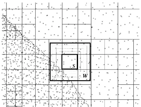
in-Fig. 1. Segmentation of lidar data using quadtrees. The midsize segment has 484 grid points to be interpolated using the points within the segmentSand its neighborhood, defined by the “growing window”W.
tractable for large datasets typical for lidar surveys. The problem can be solved by applying the function locally because, at a given point (or within a small area), the function is not sensi-tive to data at some sufficiently distant location. A widely used approach, both for splines and kriging, is the neighborhood ap-proximation, in which a separate function is computed for each grid point using points in its neighborhood, with usu-ally between 12–24 [10]. This approach may lead to minor dis-continuities in the resulting surface that are visible in the aspect and curvature maps.
Alternatively, it is possible to apply the approximation func-tion within a segment of a grid using the points located within this segment and additional points from its neighborhood. If the data points have a heterogeneous spatial distribution, the decom-position into segments with approximately the same number of points can be done efficiently using quadtrees. The quadtree has all data points stored in its leaf nodes in such a way that each leaf’s array has no more than points and the union of all rectangles defined by leaf nodes of is the entire region. A threshold three-dimensional (3-D) distance can be defined to identify points that are practically identical (e.g., due to the scanning overlaps), and such points are removed from the input dataset during the decomposition procedure.
automatically increased for larger segments using the following relation [18]:
(7)
where , is the width of the given segment, and is the width of the smallest segment.
To ensure the numerical stability and minimize the impact of scale on tension parameter, the distances are normalized using the average segment size , where is the area of the entire region and is the approximate number of segments (with their windows ).
The RST function has been implemented in open-source GRASS geographic information system (GIS) [16], [18] in moduless.surf.rstandv.surf.rst. It is also available for online gridding of lidar data [19].
III. APPLICATIONS
The RST method was applied to analysis of short-term coastal topographic change using two sets of lidar surveys for North Carolina, U.S. The first set is based on mapping of the coast using the Airborne Topographic Mapper II [1], [20] with ter-rain sampled from an altitude of 700 m at one point per 1–3 m density using an elliptic scanning pattern. The vertical and hori-zontal accuracy is 0.15 m (bare areas) and 0.80 m, respectively. Only the first return points were acquired, representing the ter-rain surface with vegetation and buildings. The second set in-cludes data from Floodplain Mapping Program survey 2001 [2] acquired by Leica Geosystems aeroscan with linear scanning pattern and about one point per 3-m density measured from an altitude of 2300 m. Bare ground data were available with the published vertical accuracy of 0.20 m and the horizontal accu-racy of 2 m.
A. Impact of RST Parameters on a Lidar-Based Surface
To assess the suitability of the RST function for generating DGM/DSM from lidar data an analysis of impact of its param-eters on the resulting surface geometry and accuracy was per-formed. The analysis was done for the density of points given by a minimum 3-D distance m. The DGMs and DSMs were interpolated at 1-m resolution so that the dune features used in the topographic change analysis were adequately represented.
First, smoothing was set to 0.0, and tension was changed gradually from 900 to 100. The surface passed exactly through the data points, and the root mean square of deviation (RMSD) was zero; however, the surface was noisy, including the bare sandy areas [Fig. 2(a)], and at lower tensions ( ) over-shoots were present [Fig. 2(a) insert]. Maps of gradients and curvatures derived from these surfaces were noisy and reflected the lidar scanning pattern rather than topography. Introduction of a small value of smoothing ( ) substantially improved the resulting surface while preserving the sharp features, such as dune crests [Fig. 2(b)]. The solution was without overshoots for a wide range of tension values [Figs. 3(f) and 4(a)], the noise was reduced, and topographic features emerged that are mean-ingful for applications.
Fig. 2. Impact of tension'and smoothingwon the 1999 DSM. (a)' = 400, w = 0:0. Insert shows overshoots for' = 100,w = 0:0. (b)' = 100, w = 0:1. Thewand'values are given for the RST implementation ass.surf.rst
module run with the0tflag [16].
The level of detail represented by the DSM was then set by tuning the tension and smoothing parameters [21]. For example, the surface computed with and was still noisy, but it captured what appear to be mailboxes on the edge of the road [Fig. 3(a) and (e)]. For applications that require smooth dune surface with clearly defined dune crests, a surface com-puted with and was more useful, as it allowed us to use curvatures for extraction of crests while the small fea-tures were smoothed out [Figs. 3(b) and 5]. Bare ground data from the 2001 survey had most of the small features already re-moved along with vegetation, as illustrated by the detail of the 1-m resolution DGM approximated by RST [Fig. 3(c)] and 6-m resolution DGM product derived by the standard methods that smoothed out most of the road [Fig. 3(d)].
Fig. 3. Elevation surface along the road. (a) The 1999 DSM with' = 400, w = 0:1. (b) The 1999 DSM with' = 200,w = 1:0. (c) The 2001 DGM ' = 100,w = 0:1. (d) The 2001 DGM at lower (6 m) resolution. (e) Aerial photo with highlighted driveways. (f) Relation between the tension parameter and mean absolute error (MAE) and deviation (MAD) for the road area.
had deviations lower than the published data accuracy for both DSM and DGM for almost all tested values of tension. Analysis of relationship between the tension/smoothing parameters and DSM accuracy using on-ground RTK-GPS measurements (per-formed in 2004 with 0.10-m published vertical accuracy) on a paved road showed the highest error for low-tension parameter [Fig. 3(f)]. Error decreased when tension was increased until it reached minimum for , [Fig. 3(f)]. Further increase in tension leads to slow increase in error; however, the error remains very low (less than 0.08 m) for a wide range of parameters, confirming the high accuracy of both the lidar measurements and the RST approximation method when applied to the paved road. The surface deviations decrease steadily with increasing tension, with the values below the error for most of the tested tension values. The 2001 data have higher error (RMSE MAE m), with substantially higher mean bias error (MBE) when compared to the 1999 data
(MBE m compared to MBE m).
B. Extraction of Topographic Features
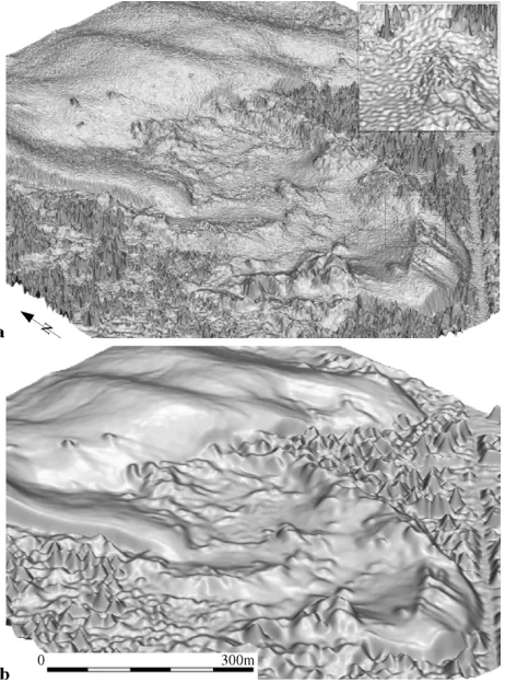
In the study of a dune field, located within the Jockey’s Ridge state park in North Carolina, U.S., the high-resolution DSM, DGM, and topographic parameters were used to extract features
Fig. 4. Deviations between the DSM, DGM (w = 0:1) and given data. (a) Relation between MAD and tension in open sand areas, areas with vegetation, and for the entire DSM, DGM. Tension. (b) Spatial distribution of deviations for DSM and DGM.
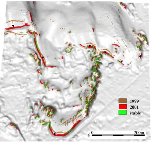
Fig. 5. Horizontal dune migration (1999–2001) represented by dune crests extracted from DSM/DGM using profile curvature draped over DGM.
Fig. 6. Assessment of change in beach morphology using profile curvature derived from 2-m resolution DSM (' = 200andw = 0:1). (a) Stable berms. Upper inset illustrates noisy pattern of curvatures for higher tension. (b) Scarp indicating rapid erosion. Inset shows change in the beach shape using a cross-section. Red line represents mean high water level.
10 m/year in some locations [17]. The slip faces were extracted as areas with slope and m, and new slip faces were identified in 2001 DGM compared to 1999 surface.
The second study used the 1998–2000 lidar data to quantify beach erosion on the Bald Head Island located near the mouth of the Cape Fear River, NC. Profile curvature, derived along with approximation of 2-m resolution DSMs, was used as an indi-cator of beach morphological change. The curvature map for 1998 beach includes a subtle pattern of parallel convex and con-cave strips, indicating the presence of berms, typical for stable beach [Fig. 6(a)]. The beach morphology significantly changed in year 2000, with higher values of slopes and curvatures and a single concave strip, typical for a beach scarp that developed due to rapid beach erosion [Fig. 6(b)]. The change in morphology was accompanied by shoreline and volume change with signifi-cant loss of sand that puts several homes into the high-risk zone.
IV. CONCLUSION
The evaluation of the RST method has demonstrated its flex-ibility and accuracy for approximation and analysis of
high-res-tuning the tension parameter. Introduction of a small value of smoothing improves stability and accuracy of the method for a wide range of tension values. Availability of the method within the open-source GIS [18] provides full access to the source code and opportunities for further improvements of its capabilities.
ACKNOWLEDGMENT
The authors would like to thank I. Kosinovsky and D. Gerdes for their contributions to the segmentation method, and D. Bernstein and C. Freeman for the RTK-GPS data.
REFERENCES
[1] NOAA. LDART: LIDAR data retrieval tool. NOAA Coastal Services Center, Charleston, SC. [Online]. Available: http://www.csc.noaa.gov/ crs/tcm/about_ldart.html
[2] State of North Carolina. North Carolina floodplain mapping program. [Online]. Available: http://www.ncfloodmaps.com/.
[3] V. R. Queija, J. M. Stoker, and J. J. Kosovich, “Recent U.S. geological survey applications of lidar,”Photogramm. Eng. Remote Sen., vol. 71, no. 1, pp. 5–9, 2005.
[4] M. E. Romano, “Innovation in lidar processing technology,” Pho-togramm. Eng. Remote Sens., vol. 70, no. 11, pp. 1201–1206, 2004. [5] J. W. Woolard and J. D. Colby, “Spatial characterization, resolution, and
volumetric change of coastal dunes using airborne LIDAR: Cape Hat-teras, North Carolina,”Geomorphology, vol. 48, pp. 269–287, 2002. [6] S. A. White and Y. Wang, “Utilizing DEM’s derived from lidar data to
analyze morphologic change in the North Carolina coastline,”Remote Sens. Environ., vol. 85, pp. 39–47, 2003.
[7] B. J. Luzum, K. C. Slatton, and R. L. Shrestha, “Identification and anal-ysis of airborne laser swath mapping data in a novel feature space,”IEEE Geosci. Remote Sens. Lett., vol. 1, no. 4, pp. 268–271, Oct. 2004. [8] C. K. Toth, “Future trends in lidar,” presented at theASPRS Annual
Conf., Denver, CO, May 2004.
[9] M. A. Brovelli, C. Massimiliano, and L. U. Matteo, “Managing and processing LIDAR data within GRASS,” presented at the OSFS GIS—GRASS Users Conf., M. Ciolli and P. Zatelli, Eds., Trento, Italy, Sep. 2002.
[10] L. Mitas and H. Mitasova, “Spatial interpolation,” inGIS: Principles, Techniques, Management and Applications, P. Longley, M. F. Good-child, D. J. Maguire, and D. W. Rhind, Eds. New York: Wiley, 1999, pp. 481–492.
[11] J. Hofierka, J. Parajka, H. Mitasova, and L. Mitas, “Multivariate inter-polation of precipitation using regularized spline with tension,”Trans. GIS, vol. 6, pp. 135–150, 2002.
[12] M. Abramowitz and I. A. Stegun,Handbook of Mathematical Func-tions. New York: Dover, 1964, pp. 228–231.
[13] H. Mitasova and L. Mitas, “Interpolation by regularized spline with ten-sion: I. Theory and implementation,”Math. Geol., vol. 25, pp. 641–655, 1993.
[14] B. K. P. Horn, “Hill shading and the reflectance map,”Proc. IEEE, vol. 69, pp. 14–47, 1981.
[15] H. Mitasova and J. Hofierka, “Interpolation by regularized spline with tension: II. Application to terrain modeling and surface geometry anal-ysis,”Math. Geol., vol. 25, pp. 657–667, 1993.
[16] M. Neteler and H. Mitasova,Open Source GIS: A GRASS GIS Approach, 2nd ed. Dordrecht, The Netherlands: Kluwer, 2004, p. 401. [17] H. Mitasova, M. Overton, and R. S. Harmon, “Geospatial analysis of
a coastal sand dune field evolution: Jockey’s Ridge, North Carolina,”
Geomorphology, to be published.
[18] GRASS GIS [Online]. Available: http://grass.itc.it/.
[19] ASU. GRASS-based LiDAR processing project. Arizona State Univ. Active Tectonics Group, Tempe, AZ. [Online]. Available: http://agassiz.la.asu.edu:8080/lservlet.
[20] H. F. Stockdon, A. H. Sallenger, H. J. List, and R. A. Holman, “Estima-tion of shoreline posi“Estima-tion and change using airborne topographic lidar data,”J. Coastal Res., vol. 18, pp. 502–513, 2002.