Stochastics Volatility Corrections for Interest Rate Models

Abstract

DAI, JIN. Stochastic Volatility Corrections for Interest Rate Models. (Under the direction of Dr. Jean-Pierre Fouque)

Stochastic Volatility Corrections

for Interest Rate Models

by

Dai, Jin

A thesis submitted to the Graduate Faculty of North Carolina State University

In partial fulfillment of the Requirements for the Degree of

Master of Science

Applied Mathematics Raleigh

2002 APPROVED BY:

Biography

Jin Dai, who earns Master degree in August 2002, is a graduate student in Mathematics Department, North Carolina State University. Her major is Applied Mathematics with specialty of financial mathematics. And her advisor is Dr. Jean-Pierre Fouque.

TABLE OF CONTENTS

List of Figures...iv

I. Introduction...1

II. Vasicek Model ...4

1. Bond Prices ...5

2. Bond Option Price...7

III. CIR Model...9

1. Bond Prices ...12

2. Bond Option Prices ...15

IV. Stochastic Volatility CIR model ...18

1. Two Factor Model...18

2. Correction for Bond Prices ...20

3. Numerical Solutions...28

4. Corrections for Bond Option Prices...31

5. Appendix ...40

List of Figures

1. Bond prices (top) and Yield curve (bottom) in the Vasicek model with a =1, 1

. 0 *=

r and σ=0.1. Maturity τ runs from 0 to 30 years. R_∞ =0.095 and the initial rate is x=0.07… … … 4 9 2. Bond prices (top) and Yield curve (bottom) in the CIR model with a =1, r* =0.1

and σ=0.1 as in Figure 1. Maturity τ runs from 0 to 30 years and the initial rate is x=0.07… … … 5 0 3. Top: bond prices (solid curve) and corrected bond prices (dotted curve). Bottom:

yield curve (solid curve) and corrected yield curve (dotted curve) in the simulated CIR model (constant and stochastic volatility) with a=1, r*=0.1 and σ=0.1 as in Figure 1. Concerning the correction we have used test parameter values

α =1

V which assumes a nonzero skew, α=5 and maturity τ funs from 0 to 30 years and the initial rate is x=0.07 … … … 5 1 4. The same assumption as in Figure 3, only has the difference that α=50… … … …

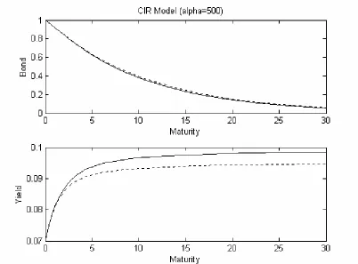
… … … 5 2 5. The same assumption as in Figure 3, only has the difference that α=500… … …

I.

Introduction

In the financial market, we will meet lots of interest rate derivatives, such as Treasure bonds, Commercial papers, Repurchase agreement, European/American bond options. How to price these derivatives is a big project attracting researchers who have tons of interests in developing the pricing skills.

The issue of pricing interest-rate derivatives has been addressed by the financial literature in a number of different ways. One of the most popular approaches is based on modeling the evolution of the instantaneous spot interest rate (shortly referred to as “short rate”) . For example, Vasicek model by Vasicek, O. (1977), Cox-Ingersoll-Stephen (CIR) model by John C. Cox, Jonathan E. Ingersoll, Jr., Stephen A. Ross (1985). In this paper, I will introduce these two models and the corrected CIR models to price interest rate

derivatives. The zero coupon bond with maturity dateT , which is also called a T-bond, a contract guaranteeing the holder 1 dollar to be paid on the date T , will be priced mainly by the models (and also the European bond option). The price at time t of a bond with maturity date T is denoted by P

( )

t,T .

where W_t is a Wiener process, µ and σ are given deterministic functions. The function

( )

t,rt

σ is known as the volatility of rt, while µ

( )

t,rt is mean of rate here.

Some well-known standard models are

• Vasicek model

(

t

)

t

t ar r dt dW

dr = * − +σ

which has the property of being mean reverting and an explicit formula for European bond options;

• CIR (Cox-Ingersoll-Ross) model

drt =a

(

r∗−rt

)

dt+σ rtdWt*

where the model is based on an ATS(Affine Term Structure) which extremely simplifies the analytical and computational method and is efficiently used now.

Note: The parameters in these models will be interpreted in the later section.

and rational expectations. From those specific formulas for interest rates and bond prices, CIR model is well suited for empirical testing.

II.

Vasicek Model

Vasicek model in this chapter will just be introduced as non-corrected model, which is one-factor and no stochastic process adding to this model. It has constant volatility. In this model, there is the probability space

(

Ω,F,P*

)

equipped with an increasing

filtration

( )

F_{t t≥0}, where _P* _{is an equivalent martingale (pricing) measure, and, the}

mean-reverting Gaussian stochastic process

( )

r_{t t≥0} is the corresponding short-rate on this risk neutral probability space.

It will follow the model

(2) dr_t =a

(

r∗−r_t

)

dt+σdW_t*,

where

( )

W_t* is a standard P*-Brownian Motion and σ is the constant volatility. In other

words, in the risk-neutral world _P*_{, the short rate}

( )

t

r is an Ornstein-Uhlenbeck process

1.

Bond Prices

Under the no-arbitrage circumstance, the bond price at time t of zero-coupon bond maturing at time T is given by

(3)

( )

   

  ∫ =

Λ − rds _t

F e

E T t

T t s

*

, .

At time 0, we can discount from t to 0 also:

( )

( )

   

  ∫ =

Λ ∫ =

Λ rds − rds _t

F e

E T t e

T

T s t

s ₀

0 _, *

,

0 .

Suppose

(4) Λ

( ) (

t,T =Pt,r_t;T

)

, r_t = x is the current short rate,

According to the Feynman-Kac formula, by the stochastic differential equation (2),

(

t x T

)

P , ; should be the solution of the partial differential equation

(5)

(

)

0

2

1 _*

2 2

2 − =

∂ ∂ − + ∂ ∂ σ + ∂ ∂

xp x P x r a x

P t

P

,

with the terminal condition P

(

T,x;T

)

=1.

The terminal condition is transferred to initial condition A

( )

0 =1 and B

( )

0 =0. Then the differential equation (5) can be solved explicitly

(7)

( )

( )

(

)

              − σ + − − τ − = τ − = τ τ − τ − ∞ ∞ τ − 2 3 2 1 4 1 exp 1 a a a e a a e R R A a e B where 2 2 2a r

R_∞ = ∗− σ is the interest rate when T goes to infinity.

The zero-coupon bond price is Λ

( ) (

t,T =Pt,r_t;T

)

with

(8)

(

)

(

) (

)

( )

(

( )

)

              − σ + − − − − − = − − − − ∞

∞ ₃ 2

2 1 4 1 exp ;

, aT t

t T a e a a e x R t T R T x t P ,

The yield, defined by

( )

(

( )

tT

)

t T T t

R , 1 log Λ ,

− −

= ,

is correspondingly solved as

(9)

(

)

(

)

( )

(

)

3

(

)

(

( )

)

2

2 1 4

1

, aT t _e aT t

t T a t T a e x R R t T t

R − −

− − ∞ ∞ − − − ₋ + σ ₋ − = − ,

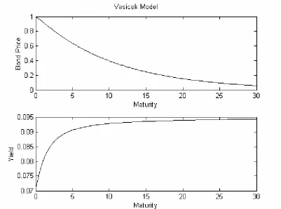
This is the explicit solution for bond price and yield, so we can obtain the figure of them directly.

2. Bond Option Price

We continue to denote the maturity of the bond by T and the maturity of a European option written on that bond is denoted by T₀ with t≤T₀<T. The payoff function is defined by h

(

Λ

(

T₀,T

)

)

, which is related with the bond price at the expiration time of the option. We write the payoff as h

(

Λ

(

T₀,T

)

)

=

(

Λ

(

T₀,T

)

−K

)

+, and it is also the function of

0

T

r , which can be presented as

( )

0

~

T

r

h . Using the Markovian structure, we denote by

(

t,x;T,T0

)

Q the price of the option at time t for an observed interest rate r_t = x and we obtain

(

)

(

(

)

)

( )

   



 _{∫ =}

=    



 _{∫ Λ =}

=E e− h T T r x E e− h r r x

T T x t

Q rds _t rds _{T t}

T t s T

t s

0 0

0 _~

, ,

;

, *

0 *

0 .

By Feynman-kac formula, it is also the solution of the partial differential equation (5) with terminal condition Q

(

T₀,x;T,T₀

) ( )

=h~ x =h

(

P

(

T₀,x;T

)

)

where P

(

T₀,x;T

)

is figured out by (8) at t=T₀.

Under the no-arbitrage world, the random variable pair 

∫

0 

0,

T t s T r ds

In the particular case, for a European call option, denoting the price of the option by

( )

t x

C , , we obtain

(10) C

( ) (

t,x = Pt,x;T

) ( )

N h₁ − KP

(

t,x;T₀

) ( )

N h₂

where N is the Ν

( )

0,1 cumulative distribution function, and h_1,2 are given explicitly by

(

)

(

)

( )

(

₂

)

(

( )

)

2

3 2 2

2

0 2

, 1

1 1

2

2 1 log ;

, ; , log

0 t aT t

T

a _e

e a

K T

x t P

T x t P h

− − −

− ₋

− σ = υ

υ

υ ± −

  



= _.

III.

CIR Model

CIR mode l is first presented by J. C. Cox, J. E. Ingersoll, Jr., and S. A. Ross in 1985. It is an equilibrium asset pricing model to study the term structure of interest rates. In this model, anticipations, risk aversion, investment alternatives, and preferences about the timing of consumption play roles in determining bond prices. And this model leads to specific formulas for bond prices, which are well suited for empirical testing.

In this section, I will give the correction form of CIR model, which will fit better for the empirical data. The idea of this correction is just introducing a new ergodic Markov diffusion process with a unique invariant distribution. The interest rates will change definitely because of the stochastic variable.

Now, first of all, the CIR model is described as followed, (11) dr_t =a

(

r*−r_t

)

dt+σ r_tdW_t*.

Here, a>0 determines the rate of mean-reversion adjustment, _r* _{is long-term mean}

level of

( )

r_t , and,

( )

* t

The interest rate behavior implied by the structure has the following empirically relevant properties:

• Negative interest rates are precluded.

• If the interest rate reaches zero, it can subsequently become positive

• The absolute variance of the interest rate increases when the interest rate itself increases.

• There is a steady state distribution for the interest rate.

Also

( )

rt cannot reach zero if ar* ≥σ2 2. The upward drift is sufficiently large to make

the origin inaccessible. In this case, the singularity of the diffusion coefficient at the origin implies that an initially nonnegative interest rate can never subsequently become nega tive. This is shown by the proposition presented.

Proposition Define τ =inf

{

≥0 x =0

}

t x

t t r , the SDE has the form

(

t

)

t t

t ar r dt rdW

dr = *− +σ ,

where

( )

Wt is a standard Brownian motion defined on

[

0,∞

)

, r0 = x>0.

For all x>0, if ar* ≥σ2 2, then P

(

τ₀x =∞

)

=1 and the solution r_t is strictly positive for all t>0.

Proof: (Outline)

Let s be the function defined on

[

0,∞

)

by

( )

₌

_∫

x σ − σ ar

ay _{y dy}

e x s

1

2

2 2 * 2 _,

And we can prove it satisfies

(

)

0

2

* 2 2 2

= −

+ σ

dx ds x r a dx

s d

x .

For ε<x<M, we set x M x x

M = τ ∧τ

τ_{ε, ε} , for any t>0, we have

( )

_∫

ε

( )

ε

τ ∧ τ

∧ _= + ′ σ

 

 x

M x

M

t

s x s x s x

t s x s r r dW

r

s ,

, 0

.

One thing need to deduce, taking the variance on both sides and using the fact that s′ is bounded from below on the interval

[ ]

ε,M , that

( )

τ_εx < ∞

M

E _, , which implies

that τ_εx_,M is finite a.s..

Then if ε<x<M, s

( ) ( )

x =s ε P

(

τ_εx <τx_M

)

+s

( )

M P

(

τx_ε >τ_Mx

)

.

We assume _ar*≥σ2 2_{, and have}

( )

=−∞ → s x x 0

lim . Deduce that

(

τ₀x <τ_Mx

)

=0

P for all M >0, then that P

(

τ₀x <∞

)

=0.

Now we assume that 0≤ar* <σ2 2 and we set s

( )

0 =lim_x→0s

( )

x , for all

x

1.

Bond Prices

The value of no-arbitrage price at time t of a zero-coupon bond maturing at time T , is similar as the bond price in Vasicek model

( )

   

  ∫ =

Λ − t

ds r

F e

E T t

T t s *

, ,

and as the function of the current short rate r_t, we similarly denote this bond pricing function by P

(

t,x;T

)

with the current rate r_t = x. It becomes

( ) (

t,T =Pt,r_t;T

)

Λ .

From the Feynman-Kac formula, P

(

t,x;T

)

is the solution of the partial differential equation

(12)

(

)

0

2

1 _*

2 2

2 _{− =}

∂ ∂ − + ∂ ∂ σ + ∂ ∂

xp x P x r a x

P x t

P

with terminal condition P

(

T,x;T

)

=1.

Let t=T−τ, we assume that the bond price has the form with initial condition

(13)

(

) ( )

( )

( )

( )

    

= =

τ = τ

− − τ

0 0

1 0 ; ,

B A

e A T x T

P B x

The partial differential equation (12) will be transformed to the new equation

(14)

(

)

0

2

1 _*

2 2

2 − =

∂ ∂ − + ∂ ∂ σ + τ ∂ ∂ − xp x P x r a x P x P .

Apply (13) into (14), we can get the following PDEs

( )

( ) ( )

( ) ( )

( ) ( )

( ) ( ) ( )

    = τ − τ τ + τ τ σ + τ ′ τ = τ τ + τ ′ 0 2 1 0 2 2 * A B aA B A B A B A ar A

By some computation for this PDE, A

( )

τ and B

( )

τ are obtained by elementary method of solving equations (15)

( )

₍

₎

₍

(

)

₎

( )

₍

₎

(

₍

)

₎















θ

+

−

+

θ

−

=

τ













θ

+

−

+

θ

θ

=

τ

θτ θτ σ θτ τ + θ

2

1

1

2

2

1

2

2 * 2 2

e

a

e

B

e

a

e

A

ar a

, θ= a2+2σ2 .

Then we have the bond price

(16)

(

)

( )

(

)

(

)

( )

( )

(

)

x

e a e ar a e e a e T x t

P θ+ − + θ

− − σ θτ τ + θ _θτθτ       θ + − + θ θ

= 1 2

1 2 2

2 * 2

2 1 2

; ,

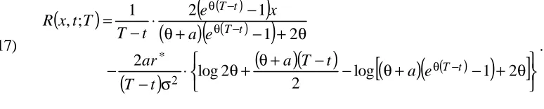
(17)

(

)

( )

(

)

(

)

(

)(

)

[

(

)

(

( )

)

]



 



 _θ+ θ+ − _{− θ+ − + θ}

⋅ σ − −

θ + − +

θ −

− θ −

θ

2 1 log

2 2

log 2

2 1

2 *

t T t

T

e a t

T a t

T ar

e a t

T

.

As we consider longer and longer maturities, the yield of bonds, which is given

by

(

)

a ar t

x R

+ θ =

∞ 2 *

;

, , approaches a limit independently of the current interest rate.

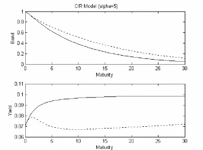
Figure 2 shows the price function and the yield curve of zero-coupon bonds under CIR model.

2.

Bond Option Prices

Use the same valuation framework of bond prices, we can easily apply to other securities whose payoffs depend on interest rates, such as bond options. Continuously, We will denote the maturity of the bond by T and the maturity of a European option written on that bond by T₀ with t≤T₀ <T .

The payoff of the bond option at time T₀ is a function h

(

Λ

(

T₀,T

)

)

, which is the bond price at expiration moment of the relative option. We will discuss a call option of the bond with striking price K and expiration time T₀ as payoff

(

)

(

_{ΛT T}

)

₌

(

_Λ

(

_{T T}

)

_−K

)

+

h ₀, ₀, .

The no-arbitrage price of the bond option is obtained by evaluating the expectation of discount value of payoff function that is under the measure _P*_{. Since the bond function}

(

T₀,T

)

Λ can be regarded as the function of rate

0

T

r from the bond price formula (16), the

payoff function is just

( )

0

~

T

r

h of the rate at time T₀. By this structure, we use

(

t,x;T,T0

)

Q to express the bond option price from an observed short rate r_t = x,

(

t x T T

)

=E e−∫ h

(

Λ

(

T T

)

)

r = x

Q rds

T t s

0

, ,

;

In the particular case of a call option, we can present the bond option price by C

( )

t,x . Here we must give that the probability density of the interest rate at time s, conditional on its value at the current time t, is provided by

(

)

2

(

( )

12

)

2

, ;

, I uv

u v e c t r s r f _q q v u t s       ⋅ = − − _, where ( )

(

)

( ) , 1 2 , , , 1 2 2 * 2 − σ α = = = − σ α = − α − − α − r q cr v e cr u e c s t s t t s

and I_q

( )

⋅ is the modified Bessel function of the first kind of order q. The distribution function is the noncentral chi-square, χ2

[

2cr_s;2q+2,2u

]

, with 2q+2 degrees of freedom and non-central parameter 2u

(19)

( )

(

)

(

)

( )

_{( )}

0 0

2 2

2 2

log

1 2

2

T B K

T A r

a e a

t T

   

 

   

  =

σ θ + = ψ

− σ

θ =

φ

σ + = θ

− θ

.

IV.

Stochastic Volatility CIR model

In this section, we will introduce a new stochastic process into the CIR model for bond and bond option prices and correct the CIR formula to include some uncertain volatility. The assumption of the volatility is fast mean-reverting with respect to the long time-scale of derivative contracts.

1.

Two Factor Model

In the real world, the yield curve is not simply a smooth curve and the real interest rate is vibrated. Therefore, let us introduce an ergodic Ito diffusion process

( )

Y_t with a unique invariant distribution

  

 Ν

α β 2 ,

2

m , and replace the diffusion of r_t by the stochastic

volatility σ

(

r_t,Y_t

)

.

Assume that under the risk-neutral world _P*_{, we have the two-factor model, which the}

(20)

(

)

( )

(

)

(

)

   

ρ − + ρ β + −

α =

+ − =

* 2 *

* *

1 t

t t t

t t

t t t t

t

dZ dW

r dt Y m r dY

dW r Y f dt r r a dr

,

where

( )

* t

W and

( )

* t

Z are two independent standard _P*_{-Brownian Motion,}

( )

t

Y f is a positive function regarding as the stochastic volatility with 0<c₁≤ f ≤c₂<∞ for some constants c₁ and c₂. And the proposition in page 10 guarantees existence of a strong

solution for

( )

r_t if f2

( )

y ≤2ar*.

The parameter ρ with ρ <1 allows a correlation between the Brownian motion

( )

W_t* driving the short rate and its volatility. Especially, we could assume ρ>0 as rising volatility trends to push bond prices down, and correspondingly, yields up.

2.

Correction for Bond Prices

By the previous section about bond price with respect to CIR model, we can learn that the bond pricing function P

(

t,x,y;T

)

is measured under x=r_t and y=Y_t, which is

(21)

(

)

      _{∫ = =}

=E e− r xY y

T y x t

P rds _{t t}

T

t s ,

; ,

, *

where the expectation E* under the risk-neutral world is related with the distribution of

(

rt,Yt

)

which is solved from the CIR model starting at time t from

( )

x,y .

Using the same framework, by two-dimensional Feynman-Kac formula, we have the partial differential equation

(22)

(

)

(

)

( )

( )

0

2 1 2 1 2 2 2 2 2 2 2 * = −       ∂ ∂ β + ∂ ∂ ∂ βρ + ∂ ∂ +       ∂ ∂ − α + ∂ ∂ − + ∂ ∂ xP y P x y x P x y f x P x y f y P y m x x P x r a t P

with terminal condition P

(

T,x,y;T

)

=1,∀x,y.

(23)

(

) (

)

, 1 1 , ; , , ; , , , 2 , 1 2 1

0 L L

L L T y x t P T y x t P + ε + ε = = ε ν = β α = ε ε ε where

(24)

(

)

    ∂ ∂ − + ∂ ∂ ν = y y m y x L 2 2 2 0

is the infinitesimal generator of the Ito diffusion process

( )

Y_t scaled by x α,

(25)

( )

y x y xf L ∂ ∂ ∂ νρ = 2

1 2 ,

and

(26)

( )

(

)

1

2 1 _* 2 2 2 2 x x x r a x x y f t L − ∂ ∂ − + ∂ ∂ + ∂ ∂ =

is the CIR operator with volatility f

( )

y and long run mean _r*_.

The partial differential equation can be written as

(27) LεPε =0,

with the terminal condition Pε

(

T,x,y;T

)

=1.

Now we want to find an asymptotic solution of the form

Note: Using this probabilistic representation, which the equation should be satisfied with the error and the regularity of the approximation, we will apply the theorem in Appendix in this section.

Zero-order term

Look at the equations at each order starting with the highest order Ο

( )

ε−1 which easily obtain from the expansion

0

0 0P =

L .

Then we can deduce

(

t x T

)

P

P₀ = ₀ , ; which does not depend on y.

Note: This conclusion cannot be deduced directly from the generator operating on the variable y only. It should be obtained from the original part of expansion

(

)

0 0

2 0 2 2 0

0 _∂ =

∂ − + ∂ ∂ ν =

y P y m y

P P

L ,

The solution of this ODE is

(

t xT

)

c

(

t xT

)

e( ) du c

(

t xT

)

P y

u m

; , ;

, ;

, _{1 2}

0 2

2

+

=

_∫

∞

− ν

−

For the bond price P₀

(

t,x;T

)

, it is impossible that P₀ goes to infinite. Thus, we

can understand the term of

(

)

( )

du e

T x t

c y

u m

∫

−∞ ν −

2 2

; ,

1 should be zero, i.e.,

(

, ;

)

0

1 t xT =

c .

Therefore, we have P₀ =P₀

(

t,x;T

)

.

The 

    

ε

Ο 1 _{terms give}

0 0 1 1

0P +L P =

L

⇒ P₁ =P₁

(

t,x;T

)

This is because P₀ does not depend on y from the previous conclusion and L₁ takes derivatives with respect to y. So, we obtain that P₁=P₁

(

t,x;T

)

also does not depend on

y . This result is very important because the present value Y_t = y of diffusion

( )

Yt is no

need for the first correction to P₀.

The Ο

( )

1 terms show us

0

0 _{2 0 0 2}

2 0 1 1 0

2P +L P +L P = ⇒L P +L P =

L

with respect to the Gaussian density, i.e. the solvability condition is L₂P₀ =0.

Since P₀ does not depend on y , it can be out of the brackets

(29)

(

)

0 2 1 0 * 2 2 2 0 2 0 2 =     − ∂ ∂ − + ∂ ∂ σ + ∂ ∂ = = P x x x r a x x t P L P L

with P₀

( )

T,x =1 and σ2= f2 .

Note: ⋅ means the averaging with invariant distribution of

( )

Y_t .

Equation (29) is similar to the equation by one-factor affine CIR model, changing the variable τ=T−t for convenience, we get

(30)

(

) ( )

( )

( )

₍

₎

₍

( )

₎

( )

₍

₎

(

₍

)

₎

2 2 2 2 0 2 2 1 1 2 2 1 2 ; , 2 * σ + = θ θ + − + θ − = τ     θ + − + θ θ = τ τ = τ − θτ θτ σ θτ τ + θ τ − a e a e B e a e A e A T x T P ar a x B .

First-order term

The Ο

( )

ε terms

(31) L₀P₃ +L₂P₁+ L₁P₂ =0,

which is also a Poisson equation in P₃ with solvability condition L₂P₁+L₁P₂ =0

By previous description L₀P₂+ L₂P₀ = 0 and L₂ P₀ =0, we have

(

L P L P

)

k

( )

t x L

P₂ =− −₀1 _{2 0}− _{2 0} + , , where k

( )

t,x does not depend on y. Then we can rewrite equation

(

)

0

0 2 2 1 0 1 1

2 ~

P

P L L L L P

L

D &

=

− ε

= −

,

with zero terminal condition at t=T.

The operator L₂− L₂ is given by

( )

(

)

2₂

2 2 2

2

2 1

x f y f L

L

∂ ∂ −

Now introduce a centered function Φ, such that L

(

f

( )

y 2 f 2

)

x

0Φ= −

Then,

(32)

(

)

( )

3₃ 3₃

2 2 1 0 1

2 f y y x x V x x

L L L L ∂ ∂ ⋅ = ∂ ∂ ∂ Φ ∂ ρ α ν = − ε = − & D

where ρ Φ′

α ν

= f

V

2 .

So we have

3 0 3 0 1 2 ~ x P Vx P P L ∂ ∂ =

=D .

Note: If no skew

(

ρ=0

)

, it implies V =0, i.e., L₂ P~₁ =0. Then the correction is just equal to P₀ itself.

Change the variable τ=T−t, the equation becomes

(33)

(

)

[

A

( )

e B( )x

]

x Vx P x x P x r a x P x

P _{− τ}

τ ∂ ∂ − = − ∂ ∂ − + ∂ ∂ σ + τ ∂ ∂ − 3 3 1 1 * 2 1 2 2 1 ~ ~ ~ 2 1 ~

with the initial condition P~₁

(

T −0,x;T

)

=0.

We now try to find a solution of the form

(34)

(

)

(

( )

( )

) ( )

( )

(

1 2

)

0 2 1

1 , ;

~ P D x D e A D x D T x T

P B x

Apply (34) into PDE (33), we can deduce to the following equation,

(

D₁′x+D₂′

)

=−σ2D₁Bx+a

(

r*−x

)

D₁+V⋅B3x, which imply the ODEs

(34)

(

)

   

= ′

+ σ − = ′

1 * 2

1 2

3 1

D ar D

D a B VB

D

,

3.

Numerical Solutions

However, we cannot find an explicit solution of (34) directly, because B is a

complicated function of τ, even by some efficient solving software such as Mathematica 4.0.

Alternatively, we use Matlab to obtain the asymptotic solution for ODEs (34). Matlab 6.0 has developed bunch of solvers to figure out the initial value problems for ordinary differential equations, which is mainly ode45, ode23, ode113, ode15s and ode23s.

We should also observe that (34) is a stiff problem, so we pick up the ode15s and ode23s, which are developed to solve the stiff ordinary differential equations.

ode23s is based on a modified Rosenbrock formula of order 2. Because it is a one-step solver, it may be more efficient than ode15s at crude tolerances. It can solve some kinds of stiff problems for which ode15s is not effective.

Then, we decide to choose Matlab ODE solver ode23s to solve D1&D2. The solver code is

Note: odefun---a function that evaluates the right-hand side of the differential equations; tspan---a vector specifying the interval of integration;

D0---a vector of initial conditions;

options---optional integration argument created using the odeset function to adjust the integration parameters of the ODE solvers;

parameters---optional parameters to be passed to odefun.

By this asymptotic method, the bond correction price is

(

1 D1x D2

)

P0

P= + + ,

and the yield is

( )

τ

−

= P

R ln ,

which could be obtained directly from the numerical solutions D₁&D₂.

In the Figure 2 attached, we can compare the correction bond prices and yield curves with those non-corrections’(just from the one-factor model).

[Figure 3 about here]

some tendency to decrease a little before increase, though the difference of corrected bond price and the original one is trivial, whatever the value of α. We can learn from the Figure 4.

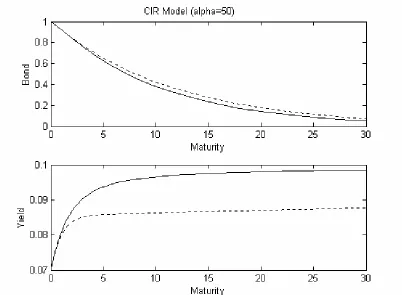
[Figure 4 about here]

When α=500 , the shape of corrected yield curve is similar with the uncorrected one, because if α goes to infinity, it means the volatility of r_t becomes constant, i.e., the uncorrected model is the same as corrected model. The Figure 5 will also show this.

4.

Corrections for Bond Option Prices

Now, we focus on the bond option prices problem in terms of this two-factor model, which introduced in previous section. The short rate process

( )

r_t and the diffusion

( )

Y_t

driving the volatility are notified by (20). We still consider the zero-coupon bond option as described above with payoff function h

(

Λ

(

T₀,T

)

)

. Under the martingale measure P*, and given the current rate r_t =x and current volatility level Y_t = y, the price of zero-coupon bond option is

(

)

(

(

)

)

   



 _{∫ Λ = =}

=E e− h T T r x Y y

T T y x t

Q rds _{t t}

T

t s , ,

, ; ,

, ₀ * ₀

0

.

Where the payoff function is coming from the bond price at time T₀,

(

)

(

)

    

   ∫ =

=

Λ − 0 _{0 0}

0

0, ; ,

,

, ₀ *

0 T T

ds r T

T Y T E e r Y

r T P T T

T

T s _.

Again, by Feynman-Kac formula, the price of bond option Q

(

t,x,y;T₀,T

)

is still the solution of partial differential equation

(

*

)

(

)

   

 

∂ ∂ − α + ∂ ∂ − +

∂ ∂

(35)

(

)

(

)

(

PT x yT

)

h

y Y x r e

E h T T y x T

Q rds _{T T}

T T s

; , ,

, ,

; , ,

0 * 0

0 0 _{0 0}

=

    

  

    

  

= =

∫

= −

where P

(

T₀,x,y;T

)

is the price of bond with current short rate x and volatility level y.

The framework for bond option price expansion is just similar to that of bond price correction. We have the bond price Pε

(

t,x,y;T

)

expanding as in notation (28),

(

)

=

(

)

+ ε

(

)

+L

ε _{t x yT P t x yT P t x yT}

P , , ; ₀ , , ; ₁ , , ;

which could be proved not to depend on y in the later part of that section.

So, we can expand the bond option price Qε

(

t,x,y;T₀,T

)

as that of bond price

(

t x y T

)

Pε , , ;

(36) Qε

(

t,x,y

)

=Q₀

(

t,x,y

)

+ εQ₁

(

t,x,y

)

+L.

Assuming that the payoff function h is smooth, by Taylor formula, the terminal condition (35) can be expanded as

(

)

=

(

(

)

)

+ ε

(

)

′

(

(

)

)

+L

ε _{T x y h P T xT P T xT h P T xT}

Q ₀, , _{0 0}, ; _{1 0}, ; _{0 0}, ;

Zero-order term

Expand the equation LεQε = 0, where Lε and correspondingly L1, L2 and L3 is

denoted as (24)-(26).

The 

     ε

1

O term is L₀Q₀ =0, which implies that Q₀

(

t,x,y

)

=Q₀

( )

t,x doesn’t depend on y.

The 

    

ε

1

O term is L₀Q₁+L₁Q₀ = 0. From Q₀ denoted as above and definition of L₁,

it is just L₀Q₁ =0, which implies that Q1

(

t,x,y

)

=Q1

( )

t,x also doesn’t depend on y .

The O

( )

1 term is L₀Q₂ +L₁Q₁+L₂Q₀ =0, which reduce to L₀Q₂ +L₂Q₀ =0. This is a

Poisson equation for Q₂ with the solvability solution L₂Q₀ = L₂ Q₀ =0. (Here Q0

can be moved out of blanket because of its independence on y. Therefore, Q₀

( )

t,x is the solution of equation

( )

(

)

0

2 1

0 0 *

2 0 2 2

0 _{− =}

∂ ∂ − + ∂ ∂ +

∂ ∂

xQ x Q x r a x

Q x y f t

Q

Consequently, Q₀

( ) (

t,x =Qt,x;T,T₀

)

represents the bond option price of CIR model. It can be written as

( )

(

(

)

)

(

)

( )

(

)

      _{∫ − =} =       _{∫ =} = − − − − x r e T T A h e E x r T r T P h e E x t Q t r T T B ds r t T ds r T T t s T t s 0 0 0 0 0 0 * 0 0 *

0 , , ;

where A and B are denoted by (30) , and

( )

r_t is the risk-neutral one-factor process with the expectation under the one -factor martingale measure _P*_.

First-order Term

The O

( )

ε term:

0 3 0 2 1 1

2Q +LQ +L Q =

L

which is also a Poisson equation in Q₃ with the solvability condition of

0 2 1 1

2Q +LQ =

L .

We can get the similar deduction about this equation from the first-order term of bond

price correction with the same notation

3 3 x x V ∂ ∂ ⋅ =

D , and ρ Φ′

α ν = f V 2 ,

( )

(

f y f

)

x

Here, we define Q~₁

( )

t,x = εQ₁

( )

t,x , the solvability condition becomes 0 1 2 ~ Q Q

L =D .

Now we write the terminal condition at time T₀,

(

T x

)

P

(

T xT

)

h

(

P

(

T xT

)

)

Q~_{1 0}, = ~_{1 0}, ; ′ _{0 0}, ; .

This is a combined stochastic Dirichlet and Poisson problem, by the corollary (p167) in [1]. We can represent the solution as the following probabilistic form

( )

(

) (

(

)

)

(

)

   = ∫ −    _{∫ ′} =

∫

− − x r du r u Q e T r T P h T r T P e E x t Q t T t u ds r T T ds r u t s T t s 0 0 0 0 , ; , ; , ~ , ~ 0 0 0 0 1 * 1 D ,

Then by (36)

( )

( )

( )

(

)

(

) (

) (

(

)

)

[

]

(

,

)

; , ; , ~ ; , , ~ , , ~ 0 0 0 0 0 0 * 0 0 0 1 0 0 * 1 0      _{− ∫ =} −       _{∫ + ′ =} = + ≈

∫

− − x r du r u Q e E x r T r T P h T r T P T r T P h e E x t Q x t Q x t Q t T t u ds r t T T T ds r u t s T t s D

price can also obtain from the expectation under risk-neutral world _P*_,

( )

(

)

_{

₍

₎

_}

(

)













_∫

₌

−













_∫

_⋅

₌

=

∫

− > −

x

r

du

r

u

Q

e

E

x

r

T

r

T

P

e

E

x

t

Q

t T t u ds r t K T r T P T ds r u t s T T t s 0 0 0 0 0 0

,

1

;

,

~

,

~

0 * ; , 0 1 * 1

D

.

From the function D₁ and D₂ numerically calculated by (34), and the formula of (18) for

( )

t x

C , , the corrected call bond price becomes (37)

( ) ( )

(

(

)

(

)

) (

)

[

( )

]

( )

_{( )}

(

)

2 1 0 * 0 2 2 * 0 2 0 0 2 0 1 0 , 2 , 4 ; 2 ; , , , I I du x r r u Q e E T B xe ar T B r T x t P T T D x T T D x t C x t C T

t u t

ds r t T u t s − =       _{∫ =} −     + ψ + φ φ σ + ψ + φ χ ⋅ − + − + =

∫

− − θ & D

where θ, ψ, φ, r are followed by (19).

For the second term I₂, it need to be presented carefully,

(38)

(

)

(

)

du x r ds r r u G E du x r r u Q r r V e E du x r r u Q e E I T t t u t s u T

t u t

u u ds r T

t u t

Here

(

)

Q

(

u r R

)

r r V e R r u

G ; , R _{3 0} ; ,

3

∂ ∂ ⋅

= −

with the variable pair r

∫

ur ds t s

u, , which has the complicated distribution. However, we can still get this distribution by Inverse Laplace Transform.

First we give out the a proposition which will help us to solve the distribution Proposition For any non-negative λ and µ, we have

(39) E e r e rdsr_t x

(

ar

(

u t

)

)

(

b

(

u t

)

)

u

t s

u = − ξ − − ζ −

      _{∫ =} µ λ µ λ µ − λ − , , * _exp exp

where the function ξ_λ,µ and ζ_λ,µ are given by

(40)

( )

( )

(

)

(

)

_         + ω + − ω + − λ σ ω σ − = ξ _{ω ω} + ω µ λ a e a e e v v v a v 1 2 log 2 2 2 2 , and

(41)

( )

(

(

)

(

)

) (

)

(

a

)

e a e e a e a v v v v v + ω + − ω + − λ σ − µ + − ω + + ω λ = ζ_{λµ ω} ω _ω ω 1 1 2 2 ,

with ω= a2 +2σ2µ .

Note: Proof can be obtained from [8], p130-131.

By the 2-dimension Laplace Transform, we have the formula of

(42)

( )

which is just the joint density function of the pair

(

r_u,_∫tur_sds

)

,

(43) f_uλµ

( )

r R =

(

(

−ar*ξ_λ,µ

(

u−t

)

)

(

−xζ_λ,µ

(

u−t

)

)

)

,

, , exp exp

-1

L ,

where ξ_λ,µ and ζ_λ,µ follow (40), (41).

Now we have the joint density function for

(

r_u,_∫tur_sds

)

, then, it is very easy to get its conditional expectation,

(

)

( )

∫ ∫

∫

= ∞ ∞ ⋅     ₌    

0 0 , ,

*

, ,

; ,

;r rds r x G u r R f r R drdR

u G

E t u

u

t s

u λµ .

If we return to (38), we can obtain I₂,

(44)

(

)

( )

∫ ∫ ∫

∫

∫

∞ ∞ ⋅ =     ₌     = 0 0

0 0 , ,

* 2 , , ; , ; T t u T t t u t s u drdRdu R r f R r u G du x r ds r r u G E I µ λ ,

where f_u,λ,µ

( )

r,R is given by (43).

Finally, we can combine the (37) and (44) together and get the formula for C

( )

t,x ,

( ) ( )

(

(

)

(

)

) (

)

[

( )

]

( )

_{( )}

(

)

( )

∫ ∫ ∫

∞ ∞ λµ − θ ⋅ −     + ψ + φ φ σ + ψ + φ χ ⋅ − + − + = 0

0 0 , ,

0 2 2 * 0 2 0 0 2 0 1 , , ; 2 , 4 ; 2 ; , , , T t u t T drdRdu R r f R r u G T B xe ar T B r T x t P T T D x T T D x t C x t C

NoncentralChiSquareDistribution[n, lambda],

which is the noncentral chi-square distribution function with n degrees of freedom and noncentrality parameter lambda.

Also, we can use the Integrate[f, x] to calculate the multiple integral in the results.

Then combine the numerical solution of D1 and D2 together, we can directly

5.

Appendix

Theorem Suppose P₀, P ,₁ P and2 P3 is given by above correspondingly. Define the

error term Z by ε

ε ε _{=P +P +εP +ε P −P}

Z 32 ₃

2 1 0

~

where Pε is the model’s bond pricing function defined above. Then for any fixed t<T , x,y∈ℜ,

(

) ( )

=Ο ε

ε _{t x y}

Z , , .

Proof: Because of the smoothness and boundness of the payoff function 1 and the boundness assumption on f

( )

y , λ

( )

y and γ

( )

y .

This follows from the standard theory of linear parabolic partial differential equations. (See Friedman 1964.) Further, solutions of the Poisson equations in

( )

1

O term and in O

( )

ε term are at most linearly growing in y , so do P₂ and

3

P .

At the terminal time T we have

(

T x y

)

(

P

(

T x y

)

P

(

T x y

)

)

Zε , , =ε ₂ , , + ε ₃ , , ,

with the terminal conditions Pε

(

T,x,y

)

=P₀

(

T,x,y

)

=1 and P~₁

(

T,x,y

)

=0, i.e.

(

)

=

( )

ε

ε _{T x y O}

Next, by the properties of

(

Pε,P₀,P₁,P₂,P₃

)

,

(

)

(

)

( )

ε = ε + + ε = − ε ε + ε + ε + = ε _ε ε ε O P L P L P L P P P P P L Z L 3 2 2 3 2 2 3 1 3 2 1 0 ,

We denote L_εZ_ε =εFε,Zε

(

T,x,y

)

=εGε where

3 2 3 2 2 2 3 1 P P G P L P L P L F ε + = ε + + = ε ε ,

This is the combined Dirichlet and Poisson problem, we can get the probabilistic representation of Zε

(

)

(

)

(

)

   = = ∫ −    ∫ ε =

∫

− ε ε − ε T

t s s t t

du r T T ds r y Y x r ds Y r s F e Y r G e E y x t Z s t u T t s , , , , , , * . Consequently

(

)

=

(

( )

+

( )

)

+

( )

ε

ε _{t x y P t x P t x O}

P , , ₀ , ~₁ ,

V.

Reference:

[1] Bernet Oksendal, (2000), Stochastic Differential Equations: An Introduction with Applications, fifth Ed., Springer -Verlag.

[2] Jean-Pierre Fouque, Peter Cotton, George Papanicolaou, Ronnie Sircar, (2001), Stochastic Volatility Corrections for Interest Rate Derivatives.

[3] John C. Cox, Jonathan E. Ingersoll, Jr., Stephe n A. Ross, A Theory of the Term Structure of Interest Rates, Econometrica, Vol 53, Issue 2 (Mar., 1985), 385-408.

[4] Damiano Brigo, Fabio Mercurio, (2001), Interest Rate Models Theory and Practice, Springer-Verlag.

[5] G.R. Grimmett, D.R. Stirzaker, (1992), Probability and Random Processes, 2nd Ed., Oxford Science Publications

[6] Tomas Björk, (1998), Arbitrage Theory in Continuous Time, 1st Ed., Oxford University Press Inc., New York

[8] Nobuyuki Ikeda, Shinzo Watanabe, (1981), Stochastic Differential Equations and Diffusion Process, 2nd Ed., Amsterdam

[9] Vasicek, O. (1977). An equilibrium characterization of the term structure, J. Financial Econ. 5: 177-188

Figure 1: Bond prices (top) and Yield curve (bottom) in the Vasicek model with 1

=

Figure 2: Bond prices (top) and Yield curve (bottom) in the CIR model with a =1, 1

. 0 *=

r and σ=0.1. Maturity τ runs from 0 to 30 years. And the initial rate is 07

. 0

=

Figure 3: Top: bond prices (solid curve) and corrected bond prices (dotted curve). Bottom: yield curve (solid curve) and corrected yield curve (dotted curve) in the

simulated CIR model (constant and stochastic volatility) with a=1, _r* =0.1 _and 1

. 0

=

σ as in Figure 1. Concerning the correction we have used test parameter values

α =1

Figure 4: Top: bond prices (solid curve) and corrected bond prices (dotted curve). Bottom: yield curve (solid curve) and corrected yield curve (dotted curve) in the

simulated CIR model (constant and stochastic volatility) with a=1, _r* =0.1 _and 1

. 0

=

σ as in Figure 1. Concerning the correction we have used test parameter values

α =1

Figure 5: Top: bond prices (solid curve) and corrected bond prices (dotted curve). Bottom: yield curve (solid curve) and corrected yield curve (dotted curve) in the

simulated CIR model (constant and stochastic volatility) with a=1, r* =0.1 and 1

. 0

=

σ as in Figure 1. Concerning the correction we have used test parameter values

α =1