Synthesis, Processing, and Characterization of Magnetic Nanoparticles for use in Bit-Patterned Media.

ABSTRACT

JOHNSTON-PECK, AARON CHARLES. Synthesis, Processing, and Characterization of Magnetic Nanoparticles for use in Bit-Patterned Media. (Under the direction of Dr. Joseph B. Tracy).

Self-assembled monolayer arrays of ferromagnetic nanoparticles (NPs) may enable future magnetic recording with areal densities in the terabits per square inch regime. A transition from conventional granular media to bit patterned media (BPM) presents numerous engineering challenges to which unsatisfactory solutions will result in read and write errors and self-erasing media. To successfully implement monolayer arrays of ferromagnetic NPs as BPM, the following are required: (1) NPs assembled into a regular pattern with

circumferential periodicity and equal spacing between bits, (2) uniform magnetic response, which requires uniform volume, shape, composition, crystalline phase, magnetic anisotropy constant and orientation of the crystal axes, (3) minimal interparticle magnetostatic

interactions, and (4) thermal stability for extended periods of time (resistance to superparamagnetism).

This dissertation presents a series of studies that address several of the

aforementioned engineering challenges. The basis of these studies is the wet-chemical synthesis of ligand-stabilized Ni, Co, and FePt NPs. Two projects examine the synthetic control of Ni(core)/NiO(shell) and Co(core)/CoO(shell) NPs and their magnetic properties. Control of synthetic reactions conditions, specifically ligand type and concentration, dictates NP size. Subsequent magnetic characterization revealed that magnetic properties and

project, the feasibility of self-assembly of NP monolayers via spin-casting and the

implementation of analytical techniques to quantitatively characterize the structure of NP monolayers was investigated. The final two projects involve incorporation of FePt NPs into alumina thin films. The alumina thin film stabilizes monolayers of FePt NPs and facilitates sinter-free phase transformation into FePt intermetallic phases. Transmission electron microscopy characterization reveals that phase transformations from the alloy into intermetallic phases strongly depend on the NP composition.

The application of analytical, structural and magnetic characterization techniques to magnetic NPs elucidated how NP synthetic and self-assembly conditions determine the material structure and properties. These studies provide solutions and insight into

Synthesis, Processing, and Characterization of Magnetic Nanoparticles for use in Bit-Patterned Media

by

Aaron Charles Johnston-Peck

A dissertation submitted to the Graduate Faculty of North Carolina State University

in partial fulfillment of the requirements for the degree of

Doctor of Philosophy

Materials Science and Engineering

Raleigh, North Carolina 2011

APPROVED BY:

_______________________________ ______________________________

Joseph B. Tracy Jon-Paul Maria

Committee Chair

________________________________ ________________________________

DEDICATION

To my parents, William and Cynthia, for their never-ending love and support.

BIOGRAPHY

Aaron Charles Johnston-Peck was born on October 11, 1984 to parents Cynthia Peck and William Johnston. For his undergraduate studies he attended Case Western Reserve University and graduated in 2007 with a B.S. in Materials Science and Engineering. Aaron then continued his education at North Carolina State University pursuing a doctorate under the tutelage of Dr. Joseph B. Tracy. In the fall of 2011 Aaron defended his thesis,

“Synthesis, Processing, and Characterization of Magnetic Nanoparticles for use in Bit-Patterned Media” and received his Ph.D. in Materials Science and Engineering from North Carolina State University. Following graduation, Aaron became a post-doctoral researcher in the field of transmission electron microscopy.

ACKNOWLEDGMENTS

I sincerely thank my advisor Dr. Joseph B. Tracy for introducing me to the fascinating world of magnetic nanoparticles and helping me grow as a researcher. His inquisitive nature provided me with an endless stream of ideas for me to pursue and helped me formulate my own hypotheses for routes of inquiry. His flexible nature allowed me to pursue my personal research interests in the field of transmission electron microscopy even if they were not central to his research goals and ambitions, for which I am grateful.

Several research groups at NCSU were very welcoming and generous with both their time and resources. I thank Dr. Jon-Paul Maria and his graduate students, Elizabeth Paisley, Peter Lam, David Hook, Michelle Casper, Hasan Akyildiz, and Nicole Estrich who provided training and assistance to me in the lab. Having access to Dr. Maria’s suite of deposition chambers and characterization tools were critical in realizing my research goals. I thank Dr. Gregory Parsons and his post-doctoral researchers, Dr. Giovanna Scarel and Dr. Christopher Oldham, for providing me samples and the benefit of their group’s expertise in atomic layer deposition. I’m very grateful to have worked with Dr. Thomas Rawdanowicz who helped me develop as an electron microscopist. His dedication and enthusiasm as a lab manager kept the transmission electron microscope facilities in great working order and as a teacher he always had useful dialogue and suggestions on all things EM related.

I thank, former groupmate, Dr. Junwei Wang for introducing to nanoparticle

chemistry and my current groupmates, Peter Krommenhoek, Mehmet Sarac, and Wei-Chen “Ivy” Wu for their support and insightful conversations on research. To my friends at

NCSU, thank you for making my time here all that more enjoyable. Finally, I thank my family for their seemingly infinite encouragement and love.

TABLE OF CONTENTS

List of Tables ... vii

List of Figures ... viii

Chapter 1. Bit-Patterned Media ...1

1.1 Introduction to Magnetic Storage Media ...1

1.2 Introduction to Bit-Pattern Media...3

1.3 Technological Challenges of Bit-Patterned Media ...4

1.4 Nanoparticles as a Bit-Patterned Media...5

1. 5 Thesis Goals and Overview ...8

REFERENCES ...9

Chapter 2. Introduction to Magnetic Materials...11

2.1 Origin of Magnetism...11

2.2 Magnetic Anisotropy ...14

2.2.1 Magnetocrystalline Anisotropy...14

2.2.2 Exchange Anisotropy...15

2.3 Superparamagnetism...16

2.4 Single Domain Limit...17

2.5 Magnetic Measurements ...19

2.5.1 Temperature Dependent Measurements ...19

2.5.2 Field-Dependent Measurements ...20

2.6 Stoner-Wohlfarth Model...21

2.7 Magnetic Materials ...23

REFERENCES ...26

Chapter 3. Self-Assembly of Nanoparticles...28

3.1 Forces Guiding Self-Assembly ...28

3.2 Self-Assembly of Nanoparticle Monolayers...32

REFERENCES ...36

Chapter 4. Thin Film Growth...38

4.1 Atomic Layer Deposition...38

4.2 Growth of Al2O3 by Atomic Layer Deposition...41

4.3 Atomic Layer Deposition of Al2O3 on Nanoparticles...42

4.4 Pulsed Layer Deposition...42

4.5 Pulsed Layer Deposition Coating of Nanomaterials...43

REFERNCES...44

Chapter 5. Transmission Electron Microscopy...46

5.1 Transmission Electron Microscopy ...46

5.1.1 Imaging Modes in Transmission Electron Microscopy ...47

5.2 Scanning Transmission Electron Microscopy ...49

5.2.1 Imaging Modes in Scanning Transmission Electron Microscopy ...50

REFERENCES ...53

Chapter 6. Size Controlled Synthesis of Cobalt Nanoparticles ...54

6.1 Introduction...54

6.2 Methods...55

6.2.1 Nanoparticle Synthesis...56

6.2.2 Structural Characterization ...56

6.2.3 Magnetic Characterization...57

6.3 Results and Discussions...58

6.3.1 Structural Properties and Cobalt Nanoparticle Growth Mechanism...58

6.3.2 Magnetic Properties ...62

6.4 Conclusions...68

REFERENCES ...70

Chapter 7. Synthesis and Structural and Magnetic Characterization of Ni(core)/NiO(shell) Nanoparticles ...72

7.1 Motivation...72

7.2 Manuscript Reprint ...73

Chapter 8. Formation and Grain Analysis of Spin-Cast Magnetic Nanoparticle Monolayers 88 8.1 Motivation...88

8.2 Manuscript Reprint ...89

8.3 Addendum...108

Chapter 9. Sinter-Free Phase Conversion and Scanning Transmission Electron Microscopy of FePt Nanoparticle Monolayers ...109

9.1 Motivation...109

9.2 Manuscript Reprint ...110

9.3 Addendum...127

9.3.1 Methods...127

9.3.2 Results and Discussion ...127

9.4 Conclusions...130

9.5 Acknowledgements...130

REFERCENCES...132

Chapter 10. Phase Transformation of Alumina-Coated FePt Nanoparticles ...133

10.1 Motivation...133

10.2 Abstract ...134

10.3 Introduction...134

10.4. Experimental Methods ...136

10.5 Results and Discussion ...138

10.6 Conclusions...143

10.7 Acknowledgments...144

REFERNCES...145

Chapter 11. Conclusions and Recommendations for Further Work ...148

11.1 Summary of Conclusions...148

11.2 Recommendations for Further Works...149

LIST OF TABLES

Table 2.1. Magnetic properties of select transition metals and metal oxides that are of interest for use in nanotechnology applications including bit-patterned media. The critical diameter is the minimal stable grain size, (60kBT/K)1/3 (τ=10 years).22 Except where noted, all data are

from reference.23...33 Table 6.1. Magnetic and structural properties of cobalt nanoparticles. The saturation magnetization (MS) values listed are those after accounting for the linear susceptibility of CoO. *Indicates this was a calculated value, rather than a value measured by SQUID...76

Table 7.1. Average Ni Core Diameter and NiO Shell Thickness ...84

Table 7.2. Saturation Magnetization and Coercivity at 2.5 K with 50 kOE or Zero-field Cooling...86 Table 8.1. Summary of Nanoparticle Sizes and Circularities ...102

LIST OF FIGURES

Chapter 2

Figure 1. Schematic temperature dependent-magnetization (M vs. T) curve of a ferromagnetic material ...28 Figure 2. Schematic field dependent magnetization (M vs. H) curve of a ferromagnetic material ...29

Chapter 3

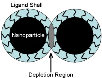
Figure 1. Schematic of an entropy-driven depletion region...40

Figure 2. Schematic of ferromagnetic nanoparticles and their associated dipoles arranging themselves into (a) rings and (b) chains, thereby reducing their magnetostatic energy ...43

Chapter 5

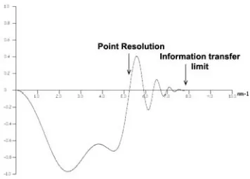
Figure 1. Simulated damped contrast transfer function ...57

Figure 2. Schematic of overlapping diffraction discs on an high-angle annular dark field detector...59

Chapter 6

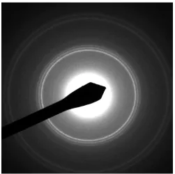
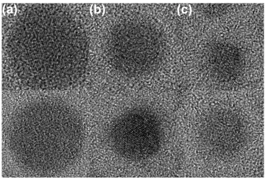
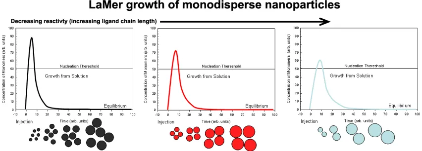
Figure 1. Bright-field TEM images of Co nanoparticles synthesized using (a) docosanoic acid, (b) dodecanoic acid, and (c) hexanonic acid ...67 Figure 2. Representative selected area electron diffraction pattern of ε-Co nanoparticles...67 Figure 3. HRTEM images of Co nanoparticles synthesized using (a) docosanoic acid, (b) dodecanoic acid, and (c) hexanonic acid ...68 Figure 4. Schematic representation of LaMer modeled growth of nanoparticles as a function of a supersaturation. The reactivity of the coordinating ligands determines the extent of supersaturation. As the ligand chain length decreases, the monomer reactivity and supersaturation increases ...70 Figure 5. Zero-field cooled magnetization as a function of temperature for Co nanoparticles synthesized using carboxylic acids with different chain lengths ...72 Figure 6. Zero- and field-cooled magnetization as a function of field measured at 5 K ...75

Figure 7. Magnetization as a function of field measured at 300 K...76

Chapter 7

Figure 1. TEM images of Ni nanoparticles: (top row) native samples; (bottom row) oxidized samples...83 Figure 2. M vs T after cooling in zero field for native and oxidized Ni(core)/NiO(shell) NPs. The inset (bottom panel) shows greater detail of the low-temperature region. Labels indicate

TB for each sample ...85

Figure 3. M vs H at 2.5 K for native and oxidized Ni(core)/NiO(shell) NPs after cooling from room temperature in 50 kOe field (FC) or zero field (ZFC). Insets show greater detail of the same measurements...86 Figure 4. Ni core-size dependence of the coercivity (zero-field cooled)...86

Figure 5. Dependence of TB on the Ni core volume. Inset shows the same plot, omitting the

two data points for samples with the largest volumes (Ni 5 and Ni 5-ox). Linear fits are shown in green ...87 Figure S-1. Photographs of the poly(lauryl methacrylate) cross-linked with ethylene glycol dimethacrylate matrix for SQUID magnetometry measurments: (left) with no nanoparticles added and (right) containing Ni(core)/NiO(shell) nanoparticles ...90 Figure S-2. HRTEM images of the native and oxidized Ni nanoparticles ...91

Figure S-3. Selected-area electron diffraction of the native and oxidized Ni nanoparticles ..92

Figure S-4. Histograms showing the distribution of total 2(rNi + tNiO) nanoparticle diameters

measured by TEM for each sample with native oxidation ...93

Chapter 8

Figure 1. (a) TEM image of Monolayer 1 of Ni nanoparticles (7.0 nm diameter) and its (b) color-coded orientation map ...100 Figure 2. Defect map of part of Monolayer 1, where defects are colored according to their coordination numbers: 4 (green), 5 (orange), 7 (cyan), 8 (magenta). Colored adjacent nanoparticles signify the presence of a defect. Examples of each type of defect have been highlighted, “V” (vacancy), “I” (interstitial), and “D” (dislocation). The oval surrounds a string of dislocations, demarcating a grain boundary ...100

Figure 3. (a) TEMimage of Monolayer 2 of FePt nanoparticles (7.2 nm diameter) and its color-coded (b) defect and (c) orientation maps and (d) Delaunay triangulation mesh. Inset (panel a): Fast Fourier transform (FFT) of the image...101 Figure 4. (a)TEM image of Monolayer 3 of FePt nanoparticles (7.2 nm diameter) and its (b) color-coded orientation map. Inset (panel a): Fast Fourier transform (FFT) of the image....101 Figure 5. TEM images of (a) Monolayer 4, a disordered monolayer of spherical FePt nanoparticles (4.2 nm diameter), and (b) Monolayer 5, a disordered monolayer of irregularly-shaped FePt nanoparticles (6.4 nm diameter). Color-coded defect maps for (a) and (b) are shown in (c) and (d), respectively. Insets (panels a,b): Fast Fourier transform (FFT) of the image...102 Figure S-1. Comparison of orientation maps for Monolayer 2 generated from Figure 3a (a) using a fast Fourier transform (FFT) mask in the process of converting the raw image to a binary image, and (b) without using the FFT mask in the conversion process. ...106 Figure S-2. Radial distribution function of Monolayer 2 (calculated from Figure 3a)...106

Figure S-3. Whole defect map of Monolayer 1, where defects are colored according to their coordination numbers: 4 (green), 5 (orange), 7 (cyan), 8 (magenta). Colored adjacent nanoparticles signify the presence of a defect. Examples of each type of defect have been highlighted, “V” (vacancy), “I” (interstitial), and “D” (dislocation). The oval surrounds a string of dislocations, demarcating a grain boundary ...107 Figure S-4. Defect map of Monolayer 3 of FePt nanoparticles (7.2 nm diameter) corresponding to the TEM image shown in Figure 4a of the main text ...108 Figure S-5. TEM image of FePt nanoparticles (6.4 nm diameter) used to synthesize Monolayer 5 (Figure 5b)...108 Figure S-6. TEM image of FePt nanoparticles (7.2 nm diameter) used to synthesize the close-packed Monolayers 2-3 (Figures 3-4) ...109 Figure S-7. TEM image of a monolayer of Ni nanoparticles (7.0 nm diameter) covering approximately 21 μm2...110

Chapter 9

Figure 1. Models of the unit cells for the different phases of FePt: (a) A1 alloy, face-centered cubic, (b) L10 FePt intermetallic, face-centered tetragonal, and (c) L12 FePt3 intermetallic, face-centered cubic ...120

Figure 2. TEM images (common scale bar) of monolayers of 4 nm FePt NPs: (a) with an Al2O3 layer, before annealing, (b) with an Al2O3 layer, after annealing (5 h at 730 °C + 3 h at 600 °C), (c) without an Al2O3 layer, after annealing (700 °C for 15 min), and (d) Al2O3-coated monolayer of 6 nm FePt NPs that sintered after heating at 900 °C for 1 h. Insets

(panels a,b): SAED ...122

Figure 3. TEM images of Al2O3-coated monolayers of (a) 5 nm and (b) 6 nm FePt NPs after annealing (5 h at 730 °C + 3 h at 600 °C). Insets (panels a,b): SAED ...122

Figure 4. TEM images of FePt NPs with diameters of (a) 5 nm, before annealing, (b) 5 nm, after annealing with Al2O3 coating, (c) 6 nm, before annealing, and (d) 6 nm, after annealing with Al2O3 coating ...123

Figure 5. XRD of an Al2O3-coated monolayer of 6 nm FePt NPs after annealing for 5 h at 730 °C + 3 h at 600 °C that converted into the L10 phase ...123

Figure 6. Filtered HAADF-STEM images with corresponding Fourier transforms (before noise filtering) and cartoons illustrating the ordering: (a) L12-FePt3 NP from the 4 nm sample, (b) L12-FePt3 NP from the 5 nm sample, and (c) L10-FePt NP from the 6 nm sample. Each NP was imaged along the [001] zone axis...123

Figure 7. Filtered HAADF-STEM images with corresponding Fourier transforms (before noise filtering) of (a,c) an A1 NP from the 4 nm sample, imaged along the [011] zone axis, and (b,d) a mixed-phase L10-FePt/L12-FePt3 NP from the 6 nm sample, imaged along the [101] zone axis. Intensity profiles acquired across the NP in panel (b) at three different points show the transition from the L12 to L10 phase...124

Figure 8. (a–c) Filtered HAADF-STEM images of 6 nmFePt NPs containing different proportions of the L10 and L12 phases, imaged along the [001] zone axis. Fourier transforms before noise filtering are shown below each NP: (d–i) selected regions corresponding to the (d,f,h) blue squares that indicate the L12 phase and to the (e,g,i) red squares that indicate the L10 phase; (j–l) for each entire NP (cropped on the top and bottom). Structure models, (m,o) simulated projected potentials, and (n,p) simulated HAADF-STEM images along the [001] zone axis for the L10-FePt and the L12-FePt3 phases are provided for comparison ...125

Figure S-1. Representative TEM image of 4.2 nm FePt nanoparticles...127

Figure S-2. Representative TEM image of 4.9 nm FePt nanoparticles...128

Figure S-3. Representative TEM image of 5.9 nm FePt nanoparticles...128

Figure S-4. EDS spectrum for 4.2 nm FePt nanoparticles ...129

xiv

Figure S-5. EDS spectrum for 4.9 nm FePt nanoparticles ...130

Figure S-6. EDS spectrum for 5.9 nm FePt nanoparticles ...131

Figure S-7. TEM image of a spin cast array of a partial multilayer of 4.2 nm diameter FePt nanoparticles ...131

Figure S-8. HAADF-STEM images used in Figure 6, before noise filtering ...132

Figure S-9. HAADF-STEM images used in Figure 7, before noise filtering ...132

Figure S-10. HAADF-STEM images used in Figure 8, before noise filtering ...133

Figure S-11. (a-b) Filtered and (c-d) the original, unfiltered HAADF-STEM images showing the presence of the FePt3 phase forming on the edges of the nanoparticles ...134

Figure 9. A plot of nanoparticle diameter versus composition. The data points in red re those nanoparticles that contain the Pt-rich L12 phase, while those in black could not have their phase identified because they were not oriented on a zone axis...137

Figure 10. Atomic resolution HAADF-STEM images of FePt nanoparticles that contain the Pt-rich L12 phase. The individual nanoparticle composition is listed with each image ...137

Chapter 10 Figure 1. TEM images (common scale bar) of monolayers of FePt NPs: (a) before deposition of Al2O3, (b) with an Al2O3layer, before annealing, (c) with an Al2O3 layer, after annealing .... ...146

Figure 2. HAADF-STEM images (common scale bar) of FePt NPs after annealing: (a) cuboctahedron along [001], (b) truncated octahedron along [001], and (c) cuboctahedron along [101]. An antiphase boundary (planar defect) is indicated in the image, and surface steps are also present...148

CHAPTER 1

Bit-Patterned Media

1.1 Introduction to Magnetic Storage Media

Hard disk drives (HDDs) used in devices such as personal computers are possibly the most recognizable and widely implemented form of magnetic storage. Magnetic storage utilizes magnetization patterns in magnetizable media to store data. In digital devices, two stable magnetic states, specifically the positive and negative remnant magnetized states, are used to encode the data in the binary numeral system of 0’s and 1’s. The first HDD became commercially available in 1956 from IBM, since then the capacity and areal density have dramatically increased while the access time, power consumption, and price have decreased drastically. To continue this trend of ever increasing areal density and associated benefits (cost reductions, faster access times, etc.) intrinsic limitations of the architecture and materials used in the fabrication of HDDs must be addressed.

HDDs consist of a platter made from a non-magnetic material that is supported on a spindle whose function is to spin the platter. The platter is coated with a thin polycrystalline film of magnetic material, in which data is stored. Read and write heads move closely over the surface of the platter and detect and modify the magnetization of the polycrystalline film. Data is encoded by orienting magnetic moments of the ferromagnetic material along specific directions. Therefore the data is stored as binary bits as a function of changes in

magnetization direction.

The ferromagnetic polycrystalline film is comprised of non-uniform grains that vary in size and crystallographic orientation. Bits are comprised of assemblies of 50-100 of these grains. The magnetic field of the write head orients the magnetic moments within the individual grains toward the applied field direction, such that the average remnant magnetization within a magnetic bit points along one of two possible directions. The boundary between each bit does not have a straight-line boundary but rather follows grain boundaries in a transition that only approximates a discrete straight line. This results in jitter (modulated noise).1 Therefore, increasing storage density by decreasing the number of grains that make up a single magnetic bit will increase noise levels because the boundary roughness becomes a greater fraction of the bit length. Consequently, the signal to noise ratio of each magnetic transition would increase preventing accurate readback and therefore is not a feasible option. An alternative approach to increase the storage density necessitates

decreasing the grain size. This route has been pursued vigorously, and present grain sizes are now approximately 8-10 nm in diameter. Further reduction in grain size is not option due to thermally induced instabilities in the magnetization of the individual grains, an effect known as superparamagnetism, whose onset is a function of volume and the magnetic anisotropy of a material. Instabilities of the magnetization directions are unacceptable because this results in data corruption.

To reiterate two significant challenges are posed that inhibit the further increases in storage density of HDDs. The current format of the magnetic media is inherently inefficient due to the fabrication process that produces a random granular film requiring collective averaging of several grains to get predictable and uniform magnetic response. The second is

an intrinsic material property limitation that becomes prevalent as grain sizes are reduced to the nanoscale. This means the architecture of magnetic storage needs to be redesigned as well as the implementation of more thermally stable magnetic materials.

1.2 Introduction to Bit-Pattern Media

Bit-patterned media (BPM) using high magnetic anisotropy materials offers a solution to both these problems. The idea of using discrete ferromagnetic entities in magnetic media and specifically BPM was suggested in the early 1990’s.2-4 BPM consists of a periodic array of discrete single-domain magnetic elements where each element functions as its own bit. Through appropriate material selection each magnetic element can have a uniaxial magnetic anisotropy. This reduces the number of possible magnetization directions to two, for

example up and down orthogonal to the plane of the substrate, which could represent 1 and 0.5 This format has numerous advantages over conventional granular media. First, in some regards the write process is simpler because the location and shape of the magnetic bit is predefined, and only the magnetization direction needs assigning. Second, transition noise is eliminated because the bits are now defined by the discrete isolated physical location of the magnetic elements and not by the contacting irregular grain boundaries in a thin film. Third, very high areal densities are achievable because the onset of superparamagnetism is

determined by the volume and anisotropy of the magnetic element representing the entire bit, rather than by individual grains that comprised the bit. Therefore, a bit can be represented by a single entity measuring several nanometers in each dimension rather than 50-100 grains

measuring several nanometers in each dimension. In BPM, bits would be smaller and could be packed more densely, allowing areal densities above 1 Terabit/in2.2-4

1.3 Technological Challenges of Bit-Patterned Media

BPM is a promising solution to overcome the insurmountable limitations of

continuous granular magnetic media. The paradigm shift of moving from granular to discrete media presents unique challenges that must be addressed before BPM can be implemented. By switching storage formats from continuous to BPD media, physical limits are traded for engineering challenges.

An important design criterion for any storage media is to minimize the occurrence of read and write errors. Understanding the origins of these errors in BPM will identify the engineering challenges of BPM. In BPM, the bits are now physically defined by the

fabrication process, whereas in conventional media, the bit positions are defined by the head position at the time when the write field is applied. This difference will manifest itself in the form of many engineering challenges because during the writing process the applied field must be synchronized with the physical location of the elements.6 _{During the read process} several sources of noise exist. These sources are due to variations in (1) bit spacing, (2) bit diameter, thickness, and shape, and (3) saturation magnetization this corresponds to a signal to noise ratio (SNR) of

2 2

1

( 7)( ) ( )

D

s D D

SNR

s D

π σ σ

=

− + 2 (1.1)

where

D

s sD

σ and σ_D D are the variations in bit spacing and size, and which are treated as Gaussians functions that are considered statistically independent.5 During the write process, as the write-head travels over the bits only during a small window of time will the intended bit be properly recorded. Deviations from this write window will result in the bit not being properly written or another bit being written instead. As a practical issue one cannot adjust the timing individually for each bit but rather an average time between dots must be defined,7 therefore necessitating periodic control of bit locations. Write-in errors are a result of (1) variations in dot spacing, (2) variations in switching field (switching field distributions of the individual bits cause variations of the writing position or times which can lead to written-in errors due to lack of synchronization due anisotropy field variations for single domain particles following the model of coherent rotation), (3) if the required switching field is larger than what the write head can apply, and (4) bit interactions (magnetostatics) changing the required switching field.6-12

These factors impose several requirements that need to be satisfied when fabricating the media. For an ideal case: First, the magnetic bits must be assembled into a regular pattern with circumferential periodicity with equal spacing between bits. Second, the

magnetic bits should have a uniaxial magnetocrystalline anisotropy axis. Third, the magnetic bits should have uniform magnetic response meaning that the volume, shape, composition, crystalline phase, magnetic anisotropy constant and orientation of the crystal axes are the same. Forth, interparticle magnetostatic interactions should be eliminated. In practice, however it is impractical (e.g. eliminating all magnetostatic interactions would limit the areal density) and unnecessary, as small levels deviations can be present without introducing

unacceptable levels of writing and reading errors. Fifth, the magnetic bits are thermally stable for extended periods of time.

1.4 Nanoparticles as a Bit-Patterned Media

Several techniques have been considered for BPM fabrication including lithography (optical, X-ray, and electron beam) and templates. Direct production of BPM by lithography depending on the specific technique used would suffer from one or multiple of the following limitations: expense, resolution limitations with respect to patterning features in the

nanometer size range, and long write times. Templating or patterning approaches using diblock copolymers or anodic anodized alumina while cost effective tend to have issues with achieving precise and reproducible long range ordering, and structures with circular

geometry has not been reported yet. Using lithography to create a master and then stamp replicas, much like how CDs are produced is another approach that shows promise but may be difficult to implement due to engineering requirements associated with the materials used in magnetic media and the feature size needed in BPM.13

Nanoparticles (NPs) provide an exciting and promising opportunity to address the engineering challenges associated with BPM. Self-assembled monolayer arrays of NPs could be implemented as the recoding media where each NP then functions as a bit. NPs have the ability to self-assemble into periodic monolayer structures. Several techniques have been reported to successfully fabricate monolayers structures with long range ordering including Langmuir-Blodgett,13 _dip-coating,14 _{spin coating,}15 _{and assembly at liquid-air interfaces with} no lateral pressures applied.16 Additionally, the presence of ligands on the NP surface

enables engineering of the assembly process and facilitates control over parameters including the packing configuration and interparticle spacing.17 Size tunable NPs can be achieved through wet-chemical synthesis with narrow size distributions (≤ 5 %).18 NP materials with applications in magnetic storage such as Co19 and high-magnetic-anisotropy materials including FePt20 and CoPt18 have been synthesized.

While immense progress in the field of NP synthesis, assembly, and magnetism has been made, significant hurdles still exist before NPs can be used in BPM. Assembly of NPs into monolayers on the wafer scale remains a challenge. While reports of patterning entire substrates with NPs exists21 these reported assemblies are closed packed in geometry and contain imperfections such as voids, point and line defects, multiple layers, and domain boundaries. Furthermore, the magnetic easy axis of the NPs when assembled through these techniques is random rather than lying along a preferred direction. Ferromagnetic NPs are susceptible to superparamagnetism. Therefore, there is a lower size limit for NPs, before they are no longer useful for BPM. To address this problem, materials must be used that have very high magnetocrystalline anisotropy such as the L10 phases of FePt or CoPt. Alternatively, exchange bias can be used to enhance anisotropy thus preventing the onset of superparamagnetism.22,23 In both cases, several engineering challenges exist.

High-anisotropy L10 NPs they are typically synthesized in the A1 phase rather than the

intermetallic phase and must be thermally treated for conversion into the intermetallic phase, which can induce sintering between NPs and a loss of their monodisperse size distribution. To implement exchange bias requires incorporation of an antiferromagnetic material.

In summary, NPs offer great promise for BPM, but additional research is needed to overcome (1) the onset of superparamagnetism, (2) uniform easy axis alignment, (3) synthetic control of NPs, and (4) scale and quality of assembly into monolayers.

1. 5 Thesis Goals and Overview

This thesis covers a series of studies that deal with the synthesis, assembly, and engineering of magnetic NPs with the explicate goal of their incorporation into magnetic storage media. Specifically, the studies here attempt to address or provide solutions to overcoming the superparamagnetic limit, synthetic control of nanoparticle properties, studies of exchange bias, as well as the self assembly of NPs.

Following this chapter on the motivations for this thesis are chapters introducing the basic science of magnetism, assembly of NPs, film growth, and characterization tools. Each project will then be presented in a self-contained chapter that covers pertinent background information, experimental methodology, results, discussions, and conclusions. Two projects examine the synthetic control of Ni and Co NPs and the subsequent control of the magnetic properties. Next a project investigates the feasibility of the formation of NP monolayers by spin-casting. Following these are two projects on the incorporation of NPs and thin films, a relatively unexplored field that holds great potential. Monolayers or multilayers of NPs incorporated into matrices provides many unique properties including extrinsic control of the NPs, high temperature stability, and many other applications not yet realized. Finally, the report will conclude with a summary of the findings and their significance.

REFERENCES

1 _{C. Jianping, H. J. Richter, W. Li-Ping, and V. B. Minuhin, Magnetics, IEEE} Transactions on 35, 2727 (1999).

2 _{T. M. Whitney, J. S. Jiang, P. C. Searson, and C. L. Chien, Science 261, 1316 (1993).} 3 _{S. Y. Chou, M. S. Wei, P. R. Krauss, and P. B. Fischer, Journal of Applied Physics}

76, 6673 (1994).

4 _{R. L. White, R. M. H. New, and R. F. W. Pease, Ieee Transactions on Magnetics 33,} 990 (1997).

5 _{C. Ross, Annual Review of Materials Research 31, 203 (2001).}

6 _{H. J. Richter, A. Y. Dobin, O. Heinonen, K. Z. Gao, R. J. M. Van der Veerdonk, R. T.} Lynch, J. Xue, D. Weller, P. Asselin, M. F. Erden, and R. M. Brockie, IEEE

Transactions on Magnetics 42, 2255 (2006).

7 _{H. J. Richter, A. Y. Dobin, R. T. Lynch, D. Weller, R. M. Brockie, O. Heinonen, K.} Z. Gao, J. Xue, R. J. M. van der Veerdonk, P. Asselin, and M. F. Erden, Applied Physics Letters 88, 222512 (2006).

8 _{M. Ranjbar, T. K. G, S. N. Piramanayagam, K. P. Tan, R. Sbiaa, S. K. Wong, and T.} C. Chong, Journal of Physics D: Applied Physics 44, 265005 (2011).

9 _{S. Yuanjing, P. W. Nutter, B. D. Belle, and J. J. Miles, Magnetics, IEEE Transactions} on 46, 1755 (2010).

10 _{P. Krone, D. Makarov, T. Schrefl, and M. Albrecht, Journal of Applied Physics 106,} 103913 (2009).

11 _{J. Kalezhi, J. J. Miles, and B. D. Belle, Magnetics, IEEE Transactions on 45, 3531} (2009).

12 _{J. Kalezhi, B. D. Belle, and J. J. Miles, Magnetics, IEEE Transactions on 46, 3752} (2010).

13 _{B. D. Terris and T. Thomson, Journal of Physics D: Applied Physics 38, R199} (2005).

14 _{D. K. Lee, Y. H. Kim, C. W. Kim, H. G. Cha, and Y. S. Kang, Journal of Physical} Chemistry B 111, 9288 (2007).

15 _{T. S. Yoon, J. H. Oh, S. H. Park, V. Kim, B. G. Jung, S. H. Min, J. Park, T. Hyeon,} and K. B. Kim, Advanced Functional Materials 14, 1062 (2004).

16 _{S. Coe-Sullivan, J. S. Steckel, W. K. Woo, M. G. Bawendi, and V. Bulovic,} Advanced Functional Materials 15, 1117 (2005).

17 _{T. P. Bigioni, X. M. Lin, T. T. Nguyen, E. I. Corwin, T. A. Witten, and H. M. Jaeger,} Nature Materials 5, 265 (2006).

18 _{S. Sun, C. B. Murray, D. Weller, L. Folks, and A. Moser, Science 287, 1989 (2000).} 19 _{C. B. Murray, C. R. Kagan, and M. G. Bawendi, Annual Review of Materials Science}

30, 545 (2000).

20 _{V. F. Puntes, K. M. Krishnan, and A. P. Alivisatos, Science 291, 2115 (2001).} 21 _{J. I. Park and J. Cheon, Journal of the American Chemical Society 123, 5743 (2001).} 22 _{A. Desireddy, C. P. Joshi, M. Sestak, S. Little, S. Kumar, N. J. Podraza, S. Marsillac,}

R. W. Collins, and T. P. Bigioni, Thin Solid Films 519, 6077 (2011).

23 _{M. N. Martin and S. K. Eah, Materials Research Society Symposium Proceedings} 1113, F03 (2009).

CHAPTER 2

Introduction to Magnetic Materials

2.1 Origin of Magnetism

The magnetic properties of a material are dictated by electron motion. Even though the nuclear magnetic moments of the nuclei exist, in a material the magnitude of those moments are negligible by comparison to the electrons’ magnetic moments and can be neglected for the purpose of discussing and understanding the macroscopic magnetic properties of bulk materials. Electrons both move around a nucleus (orbital angular

momentum) and exhibit spin (spin angular momentum). The manner in which the electrons and their associated momentums interact and align with respect to one another defines the magnetic response. Diamagnetism occurs when all the magnetic moments of all the electrons are oriented such that the vector sum of the magnetic moments is zero. For instance, filled atomic subshells will have no net moment because the electron pairs have opposite spin (Pauli exclusion principle) and the net orbital motion is also zero. Therefore every material has a diamagnetic component which manifests as a magnetic moment opposing the applied field (a linear negative magnetic susceptibility) because an applied field will increase the orbital magnetic moments of those electrons aligned opposite the field, and decreases the ones aligned parallel to the field, as described by Lenz’s Law.

However if unpaired electrons exist the diamagnetic component is negligible and the vector sum of all the moments is nonzero, the material is then para-, ferri-, ferro-, or

antiferromagnetic. If the unpaired electrons do not interact, when an external magnetic field is applied the magnetic moments align in the same direction as the applied field (a positive linear magnetic susceptibility), a response known as paramagnetism. If the unpaired

electrons interact, the material is ferri-, ferro-, or antiferromangetic. Unique to these forms of magnetism is the existence of spontaneous ordering of the magnetic moments in a solid below a critical temperature, for both ferro- and ferrimagnets, it is known as the Curie temperature (TC) and for antiferromagnets is the Néel temperature (TN). In the case of

ferromagnetism, the spins align parallel to one another, and their moments add. If the spins have antiparallel alignment and their moments cancel, then the material is antiferromagnetic. If there are two different sublattices, where the magnitudes of the opposing moments are different, then the material is ferrimagnetic. Above the Néel and Curie temperatures, magnetic ordering vanishes and the materials become paramagnetic.

This collective response of the moments is the result of exchange interactions. A direct exchange interaction occurs when electron orbitals overlap. This interaction is a quantum mechanical effect between sub-atomic particles, in this case electrons, which influences magnetic behavior.

A model can be assumed of two unpaired electrons on neighboring atoms with wavefunctions ψa(r1) and ψb(r2), where r1 and r2 indicate their positions. Because electrons are fermions and cannot occupy the same quantum state an antisymmetric wave function will be produced. Therefore either a singlet state (antisymmetric spin with a symmetric wave function) or triplet state (symmetric spin with an antisymmetric wave function) will form. The corresponding wavefunctions and energies are:

( ) ( )

( ) ( )

1 2

S ψa ψb ψa ψb S

Ψ = _⎡⎣ r₁ r₂ + r₂ r₁ ⎤⎦χ (2.1)

( ) ( )

( ) ( )

1 2

T ψa ψb ψa ψb T

Ψ = _⎡⎣ r1 r − r2 r1 ⎤⎦χ (2.2)

(2.3)

* _{d d}

S S S

E = Ψ

∫

(2.4)

* _{d d}

T T T

E = Ψ

_∫

where H is a Hamiltonian. Then taking into account the spin contributions

(2.5)

2 2 2

1 2

= ( + ) = S + S + 2 · 2

1 2 1

S S S S S₂

for which the scalar product is

3

if 0 (singlet) 4

1_{if 1 (triplet)} 4 1 3 ( 1) 2 4 total total S

total total _S

S S − =

+ =

⎧

= _{+ − = ⎨}

⎩ 1 2

S · S (2.6)

An effective Hamiltonian describing the energy can be expressed as1 1

= ( 3 ) ( )

4 S T S T

H E + E − E −E S ·S_{1 2} (2.7)

where the second half the equation is spin dependent. In order to determine which state is lower in energy, we define a term known as the exchange integral, J:

(2.8)

( ) ( )

( ) ( )

S T a b

J =E −E =

∫

If the exchange integral J is positive then the triplet state with Stotal = 1 is energetically

favored and the material is antiferromagnetic or ferrimagnetic. However if the exchange integral J is negative then the singlet state with Stotal = 0 is energetically favored and the

material is ferromagnetic. However, this model is not suitable for all types of materials due to differences in the nature of bonding within each material. Longer-range indirect exchange

(superexchange, double-exchange, RRKY exchange) is important in specific material classes (e.g., ionic compounds, metal oxides, and rare earths). Therefore multiple models are necessary to describe the different physical phenomena.

2.2 Magnetic Anisotropy

The magnetic anisotropy of a material will strongly influence its response to applied magnetic fields. There are several sources of magnetic anisotropy including

magnetocrystalline (crystalline), shape, mechanical stress, processing (annealing, deformation, irradiation), and exchange anisotropy (exchange bias).

2.2.1 Magnetocrystalline Anisotropy

Of particular importance is the magnetocrystalline anisotropy because of its intrinsic nature. Experimentally, a single crystalline material will magnetize differently along

crystallographic orientations. The crystal directions along which the moments preferentially point are called “easy” axes; the energetically unfavorable directions are called “hard” axes. This behavior has its origins in the spin-orbit interaction (an interaction of electron spin with its motion). Since electron orbitals are linked to crystal structure, the moments (spins) will tend to align along well-defined (easy) crystal axes. To switch the direction of the moments lying on an easy axis (as would occur when the direction of an applied external field is switched) a certain amount of energy is necessary, known as the magnetocrystalline energy (EA). The magnetocrystalline energy per unit volume is represented by a power series of the

form

2 sin n o a un n o E E K V θ

= =

∑

but it is generally satisfactory to discard higher order terms, thus simplifying the equation to

2 1sin

a u

E =K θ (2.10)

where Ku1is called the first magnetocrystalline anisotropy constant or when higher order

terms are neglected it is rewritten as K , the magnetocrystalline anisotropy constant. The angle between the magnetization direction and the easy axis is denoted by θ. The

magnetocrystalline anisotropy constant depends on temperature and decreases to zero upon approaching the Curie or Néel temperature, because the material becomes paramagnetic at these temperatures, and the magnetic ordering is consequently isotropic. Furthermore, the magnitude of the K can be used to separate materials into the classifications, specifically as hard or soft materials. Hard magnets have large magnetocrystalline anisotropy constants (therefore large coercivities) and soft materials have small magnetocrystalline anisotropy constants (therefore small coercivities) but often have large saturation magnetizations.

2.2.2 Exchange Anisotropy

Exchange anisotropy, also known as exchange bias, is of particular technological importance because it can increase the coercivity and superparamagnetic blocking temperature, as well as define an arbitrary unidirectional anisotropy direction in

ferromagnetic materials. It is an interfacial phenomenon, in which an exchange interaction occurs between coupled ferromagnetic and antiferromagnetic materials. Exchange bias was first reported in the Co/CoO system by Meiklejohn and Bean in 1956.2 While the

phenomenological origin of exchange bias is understood, the microscopic manner in which this exchange interaction between the spins then manifests itself into exchange bias is not thoroughly understood, and many competing models explaining this behavior exist.3-6 In simple terms, exchange bias can be described as the alignment spins at the interface of a ferromagnetic/antiferromagnetic couple. When this couple is field cooled through the Néel temperature of the antiferromagnet, the spins at the interface of both the ferromagnet and antiferromagnet will align parallel to each other. The ferromagnet is strongly exchange-coupled to the antiferromagnet and will have its interfacial spins pinned. Because

antiferromagnets generally have higher magnetocrystalline anisotropy than ferromagnets, this pinning requires extra energy to overcome and reverse the moment of the ferromagnet, which increases the coercivity. However, the pinning occurs in one direction only, and this

asymmetry causes the hysteresis loop to shift from the origin (H=0). A shifted hysteresis loop is the classical signature of exchange bias, but as previously stated, the coercivity and superparamagnetic blocking temperature of the ferromagnet can increase as well.

2.3 Superparamagnetism

Superparamagnetism is a pertinent and persistent phenomenon in the nanoscale regime because is it a volume effect. In bulk ferromagnetic materials, ordering of the moments becomes random above the Curie temperature, but in nanomaterials a transition from the ferromagnetic state to a paramagnet-like (the superparamagnetic state) can occur well below the Curie temperature. Superparamagnetism can have serious implications for products that rely on the moments of the material to be stable (e.g. magnetic data storage).

This phenomenon occurs as thermal energy (kBT) becomes comparable to the

magnetocrystalline anisotropy energy (EaV), which removes confining energy barriers and

allows the moments to fluctuate between easy axes. The average time between flips, known as the Néel relaxation time, is described by:

exp n o B KV k T τ =τ ⎛_⎜ ⎞

⎝ ⎠⎟ (2.11)

where τn is the average time between flips and τo is the material-dependent attempt frequency

with an approximate value of 10-9 s. This equation can be rewritten to give the temperature at which the material will transition from ferromagnetism to superparamagnetism. The temperature at which this occurs is referred to as the superparamagnetic blocking temperature and is defined as:

b B KV T k C ⎛ ⎞ = ⎜

⎝ ⎠⎟ (2.12)

where C=ln

(

)

(corresponds to ~ 1 min), whereas the magnetic storage industry requires C to be 50-70 (corresponds to > 10 years).7 Therefore, for the purposes of magnetic storage, it can be rewritten to estimate the magnetocrystalline anisotropy a material must possess to remain stable at given temperature for a given size

b b

T Ck K

V

= (2.13)

If one assumes room temperature, C=50, and a spherical particle of 10 nm, a material

possessing a magnetocrystalline anisotropy of greater than 1.2×106 J/m3 would be necessary.

This means that only intrinsically very hard materials or those with additional anisotropy sources, can be used for ultra-high density BPM.

2.4 Single-Domain Limit

In the previous section it was stated of ferromagnetism all the magnetic moments will point in the same direction due to the exchange interaction, but domain formation is a process that must also be considered for sufficiently large NPs and bulk ferromagnets. In the absence of a saturating applied magnetic field, a sufficiently large ferromagnetic material will not be uniformly magnetized but rather will split into domains, individual regions where all the moments align. The net moment of each individual domain will align in different directions with respect to one another. This behavior is driven by energy minimization, specifically from magnetostatics. The moments in a domain generate a dipolar field, which will tend to align moments lying side-by-side in the opposite direction. The formation of domains requires energy to form domain walls. Therefore, small NPs consist of a single domain, if

the savings in magnetostatic energy (

( )

4 9

ms s

E μ M πr

Δ ≈ , assuming a spherical particle) is

less than the energy cost associated with forming a domain wall ( 2 ₄ 2

( )

dw r r AK

σ π = π )

where Ms is the saturation magnetization and A is the exchange stiffness constant (a measure

of strength of coupling between neighboring spins). This assumes the domain wall in the NP is the same structure as that of a bulk material which is an acceptable approximation if the anisotropy of the NP is large enough to maintain the orientation of the moments along the easy axis. If the anisotropy is small, the moments will align along the surface poles and

follow the NP surface and this confinement effect increases the exchange energy contribution

and a different equation is needed. Therefore a NP with large K ( 2 0MS 6

μ

≥ ) will have a

corresponding critical radius of

1 2 2 0 ( ) 9 c S AK r M μ

≈ (2.14)

whereas a NP with small K will have a critical radius of

2 0

2 9

9 ln c

c S r A r M a μ ⎡ ⎛ ⎞ = _{⎢ ⎝ ⎠⎜ ⎟}

⎣ 1⎦

⎤

− ⎥ (2.15)

above which multiple domains will form. Calculated-single domain limits for Co, Ni, and FePt are 80, 85, and 55 nm, respectively. Therefore, all materials reported in this dissertation are in the single domain regime.8

2.5 Magnetic Measurements

2.5.1 Temperature Dependent Measurements

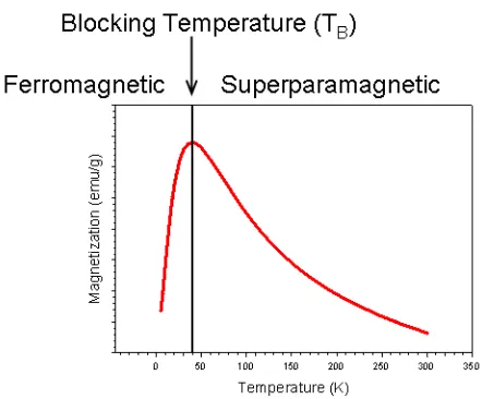
A representative M vs. T curve is shown in Figure 1. The DC measurement of magnetization (M) versus temperature (T) in a small applied field is performed on magnetic NPs in order to determine the transition temperature between ferromagnetism and

superparamagnetism. The sample is cooled in zero applied field to low temperature below the superparamagnetic blocking temperature. A small measuring field (100 Oe in our case) is applied, and the sample is heated, while measuring the magnetization as a function of specimen temperature. First, when the sample is cooled it becomes ferromagnetic as the temperature is lowered below the superparamagnetic blocking temperature. When the field

is applied, the magnetic moments are driven to align in the direction of the field due to the

Zeeman energy (E_Z = −μ₀MHV ). However, the magnetocrystalline anisotropy dominates at low temperatures and keeps the moments aligned with the randomly-oriented NPs easy axes, which gives a low measured moment. Upon heating, the increased thermal energy provides magnetic moments sufficient energy to overcome the magnetocrystalline anisotropy energy and to point toward the magnetic field direction. However, at the superparamagnetic

blocking temperature, there is a greater mean component of the fluctuating moments oriented in the field direction, which causes the magnetization to reach a maximum value. Upon further heating, the proportion of moments pointing in the applied field direction decreases, and the measured magnetization accordingly decreases. The magnetization behavior of superparamagnets obeys a Langevin function, which also describes the behavior of classical paramagnets. The temperature at which the magnetization peaks is assigned as the blocking temperature (TB).

Figure 1. Schematic temperature-dependent magnetization (M vs. T) curve of a ferromagnetic material.

2.5.2 Field-Dependent Measurements

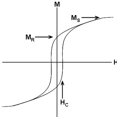
A representative M vs. H curve is shown in Figure 2. As the applied field increases, the magnetization increases when the moments align in the direction of the field. At high fields, if all the moments are aligned in the same direction, the magnetization reaches a maximum value and approaches a constant value, known as the saturation magnetization (MS). Upon decreasing the field, the moments no longer align in the same direction, but there

is hysteresis. At zero field, there remains a net magnetization, the remanace or remnant magnetization (MR). Increasing the field in the opposite direction will eventually drive the

sample’s magnetization to zero; the magnitude of this field is known as the coercivity (HC).

This process is then repeated as the loop is traversed going from negative to positive applied field or positive to negative applied field. Below the superparamagnetic blocking

temperature, the specimen will present an open loop (HC > 0), while above the

superparamagnetic blocking temperature the specimen will present a closed loop (HC = 0)

because the moments are now fluctuating causing a loss of hysteresis.

Figure 2. Schematic field dependent magnetization (M vs. H) curve of a ferromagnetic material.

2.6 Stoner-Wohlfarth Model

In bulk specimens, magnetic hysteresis is understood through domain wall motion and lossy processes known as Barkhausen jumps, as the domain walls jump between local energy minima. However, the materials studied here are single domain and do not have domain walls. Hence, another model for understanding the origin of hysteresis is necessary. In single domain NPs, the magnetic response is described by the Stoner-Wohlfarth (SW) model. The SW model assumes an ellipsoid-shaped particle with uniaxial anisotropy along the long axis. The particle is uniformly magnetized, and the moments have a strong

exchange interaction such that the moments coherently rotate (all moments change direction in unison). The magnetization can be represented by a vector M and in the absence of a field would lie along the anisotropy axis. In the presence of an applied field, the magnetization orients in a direction that would serve to minimize the energy of the system. The total energy is the sum of the magnetocrystalline anisotropy energies (EA) and Zeeman energies (EZ):

0

sin( ) cos

A Z eff s

E E= +E =K V φ θ− −μ M VH φ (2.16)

where θ is the angle between the direction of the magnetization and easy axis, while φis the

angle between the direction of the applied field and _{[ 2} 2_{( )]sin}2

eff s

K = K+ πM N_⊥−N θ

where N are demagnetization factors that are determined by the aspect ratio of the ellipsoid. This equation can be expressed using normalized variables:

(

)

1

cos 2 cos

4 h

η = − ⎡_⎣ φ θ− ⎤_⎦− φ (2.17)

where η represents the variable energy, h HM= _S 2K_eff . A stable energy minimum occurs if

0

η φ

∂ ∂ = and _∂2_{η φ∂} 2 _{>0. By solving ∂ ∂ =η φ}

( )

(

)

⎣ ⎦ φ for h as a

function of φ,a hysteresis plot can be generated.

2.7 Magnetic Materials

Storage media for BPM require a combination of several physical properties. Not only does the material need to have an intrinsically high magnetocrystalline anisotropy (or an additional anisotropy mechanism), but are also stable against oxidation and a remanent magnetization that is sufficient enough for detection. Numerous ferromagnetic materials

exist, some of which are listed with their properties in Table 1. The intermetallic L10 FePt phase is an attractive choice, owing to its high saturation magnetization and

magnetocrystalline anisotropy. However magnetic properties are not the only characteristic must be taken into consideration and as a result there currently is not an ideal material for ultra-high density BPM.

FePt NPs when synthesized by wet-chemistry techniques typically produce disordered (A1) phase or partially ordered L10, whose magnetic properties are inferior to well-ordered L10 FePt. In the L10 phase there is a large spin-orbital coupling of the Pt electrons and hybridization between theFe-d and the Pd-d states that significantly enhances the magnetocrystalline anisotropy.9 Transforming the NPs to the L10 phase while preventing sintering is a significant challenge. Moreover, the complete phase conversion from the A1 phase into the L10 phase becomes especially challenging as the size of the NP decreases.10 The bulk order-disorder reaction in FePt is first order,11 but it has been shown

experimentally12 and theoretically13,14 that it is a continuous (second order) transformation in NPs and dependent on size with the smallest dimension being the determining factor.12,15 This behavior is thought to originate from surface-induced disorder, wherein the reduced bond coordination at the surface reduces the driving forces for ordering, and configurational entropy favors a disordered NP,13,14 which has been supported experimentally.16 Furthermore chemically synthesized FePt NPs have a Gaussian-like distribution of individual NP

compositions.17,18 A substantial portion of the NPs will therefore be unable to form a

structure with perfect long range order (S = 1) since equimolar concentration is required to do

25 so. Consequently, the magnetocrystalline anisotropy will be reduced from the value expected for perfect ordering.19,20

Alternatively, unary ferromagnetic species eliminate these issues of compositional control but have lower magnetocrystalline anisotropy. Fe, Co, and Ni are susceptible to varying extents of oxidation. Fe NPs are generally unstable at room temperature and will oxidize completely, while Co and Ni NPs will form passivating oxide layers of CoO and NiO respectively. Since Co and Ni have lower magnetocrystalline anisotropy than L10 FePt, external sources of magnetic anisotropy could be considered for use to augment the intrinsic magnetocrystalline anisotropy. Enhanced anisotropy through shape control (shape

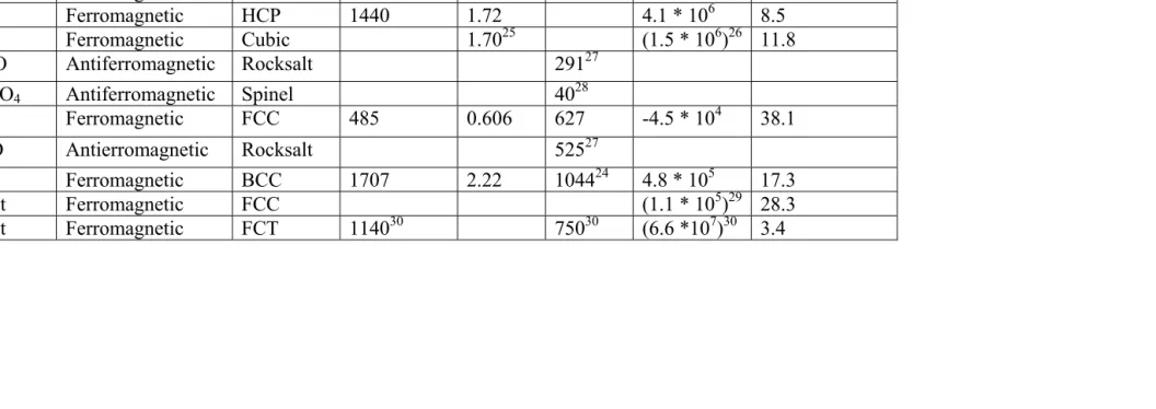
Table 1. Magnetic properties of select transition metals and metal oxides that are of interest for use in nanotechnology applications

including bit-patterned media. The critical diameter is the minimal stable grain size, (60kBT/K)1/3 (τ=10 years).22 Except where

noted, all data are from reference.23

Material Magnetic Structure Crystalline

Structure M(emu/cmS (290K) 3₎ μB T_(K) C or TN K (J/m 3_{) @}

RT Critical Diameter (nm)

Co Ferromagnetic FCC 1440 1.75 139024

Co Ferromagnetic HCP 1440 1.72 4.1 * 106 8.5

Co Ferromagnetic Cubic 1.7025 (1.5 * 106)26 11.8

CoO Antiferromagnetic Rocksalt 29127

Co3O4 Antiferromagnetic Spinel 4028

Ni Ferromagnetic FCC 485 0.606 627 -4.5 * 104 38.1

NiO Antierromagnetic Rocksalt 52527

Fe Ferromagnetic BCC 1707 2.22 104424 _{4.8 * 10}5 _17.3

FePt Ferromagnetic FCC (1.1 * 105)29 28.3

FePt Ferromagnetic FCT 114030 75030 (6.6 *107)30 3.4

REFERENCES

1 _{R. K. Nesbet, Physical Review 122, 1497 (1961).}

2 _{W. H. Meiklejohn and C. P. Bean, Physical Review 102, 1413 (1956).}

3 _{J. Nogués, J. Sort, V. Langlais, V. Skumryev, S. Suriñach, J. S. Muñoz, and M. D.} Baró, Physics Reports 422, 65 (2005).

4 _{J. Nogues and I. K. Schuller, Journal of Magnetism and Magnetic Materials 192, 203} (1999).

5 _{M. Kiwi, Journal of Magnetism and Magnetic Materials 234, 584 (2001).}

6 _{A. E. Berkowitz and K. Takano, Journal of Magnetism and Magnetic Materials 200,} 552 (1999).

7 _{C. Ross, Annual Review of Materials Research 31, 203 (2001).}

8 _{K. M. Krishnan, A. B. Pakhomov, Y. Bao, P. Blomqvist, Y. Chun, M. Gonzales, K.} Griffin, X. Ji, and B. K. Roberts, Journal of Materials Science 41, 793 (2006). 9 _{G. H. O. Daalderop, P. J. Kelly, and M. F. H. Schuurmans, Physical Review B 44,}

12054 (1991).

10 _{D. Yi and A. M. Sara, Applied Physics Letters 87, 022508 (2005).} 11 _{S. H. Whang, Q. Feng, and Y. Q. Gao, Acta Materialia 46, 6485 (1998).} 12 _{D. Alloyeau, C. Ricolleau, C. Mottet, T. Oikawa, C. Langlois, Y. Le Bouar, N.}

Braidy, and A. Loiseau, Nat Mater 8, 940 (2009).

13 _{B. Yang, M. Asta, O. N. Mryasov, T. J. Klemmer, and R. W. Chantrell, Acta} Materialia 54, 4201 (2006).

14 _{M. Müller, P. Erhart, and K. Albe, Physical Review B 76, 155412 (2007).} 15 _{W. H. Qi, Y. J. Li, S. Y. Xiong, and S. T. Lee, Small 6, 1996 (2010).}

16 _{A. Kovács, K. Sato, V. K. Lazarov, P. L. Galindo, T. J. Konno, and Y. Hirotsu,} Physical Review Letters 103, 115703 (2009).

17 _{C. C. Y. Andrew, M. Mizuno, Y. Sasaki, and H. Kondo, Journal of Applied Physics} 85, 6242 (2004).

18 _{S. Chandan, E. N. David, and B. T. Gregory, Journal of Applied Physics 104, 104314} (2008).

19 _{J. B. Staunton, S. Ostanin, S. S. A. Razee, B. Gyorffy, L. Szunyogh, B. Ginatempo,} and E. Bruno, Journal of Physics-Condensed Matter 16, S5623 (2004).

20 _{S. Ostanin, S. S. A. Razee, J. B. Staunton, B. Ginatempo, and E. Bruno, Journal of} Applied Physics 93, 453 (2003).

21 _{J. B. Tracy, D. N. Weiss, D. P. Dinega, and M. G. Bawendi, Physical Review B 72,} 064404 (2005).

22 _{D. Weller and M. F. Doerner, Annual Review of Materials Science 30, 611 (2000).} 23 _{R. C. O'Handley, Modern Magnetic Materials: Principles and Applications (John}

Wiley & Sons, Inc., New York, 2000).

24 _{H. P. J. Wijin, Magnetic Properties of Metals: d-Elements, Alloys and Compounds} (Springer-Verlag, New York, 1991).

25 _{D. P. Dinega, Thesis, Massachusetts Institute of Technology, 2001.}

26 _{V. F. Puntes and K. M. Krishnan, IEEE Transactions on Magnetics 37, 2210 (2001).} 27 _{C. Kittel, Introduction to Solid State Physics, 8th ed. (Wiley, Hoboken, NJ, 2005).} 28 _{R. W.L, Journal of Physics and Chemistry of Solids 25, 1 (1964).}

29 _{B. Stahl, J. Ellrich, R. Theissmann, M. Ghafari, S. Bhattacharya, H. Hahn, N. S.} Gajbhiye, D. Kramer, R. N. Viswanath, J. Weissmüller, and H. Gleiter, Physical Review B 67, 014422 (2003).

30 _{T. Klemmer, D. Hoydick, H. Okumura, B. Zhang, and W. A. Soffa, Scripta} Metallurgica et Materialia 33, 1793 (1995).

CHAPTER 3

Self-Assembly of Nanoparticles

Many proposed applications of nanomaterials require organization into ordered structures. It is an immense challenge to controllably arrange potentially trillions of NPs that cannot be seen or controlled using established fabrication methods. Allowing naturally occurring forces to spontaneously organize disordered NPs into ordered structures, a process known as self-assembly, is arguably the most promising method to overcome this challenge. A great deal of research has been conducted in this field, and much progress has been to improve the length scale and quality of assemblies. To fabricate these higher-ordered structures from nanomaterials in a controlled fashion requires both an understanding of interparticle interactions and the ability to modify them.

3.1 Forces Guiding Self-Assembly

Different interaction forces may exist between NPs whose magnitude and range of interaction will have implications if the NPs assemble into order structures or agglomerate into disordered arrangements. In terms of ferromagnetic ligand-stabilized NPs, the most relevant forces are van der Waals, magnetic dipole-dipole, and steric, but other forces may contribute.

Van der Waals forces originate from electromagnetic fluctuations and therefore exist between any two NPs. Van der Waals interaction can be described by three kinds of

interactions, Keesom forces (two permanent dipoles), Debye forces (permanent dipole and a

corresponding induced dipole), and London dispersion forces (two instantaneously induced dipoles). To approximate the net interaction energy, one can integrate these forces over the volumes of two NPs represented by two spheres of radii r1and r2, separated by a

center-to-center distance d1:

2 2

1 2 1 2 1 2

2 2 2 2 2

1 2 1 2 1 2

( )

1 ln

3 ( ) ( ) 2 ( )

vdW

r r r r d r r

A U

d r r d r r d r r

⎡ ⎛ − + ⎞⎤

= _⎢ + + _{⎜ ⎥}

− + − − _⎝ − − _⎠

⎣ 2⎟⎦ (3.1)

where A is the Hamaker coefficient which is equal to 2 1 2 vdW C A v v π

= (3.2)

where CvdWis a constant and v is the molar volume of a material.2 For a monodisperse

sample of NPs with radii that are approximately the same (r1≈r2), the interaction energy can

be simplified to

2 2 2 2

2 2 2 2

1 4

ln

3 4 2

vdW

A r r d r

U

d r d d

⎡ ⎛ − ⎤

= _⎢ + + _{⎜ ⎥}

− _{⎝ ⎠}

⎣ ⎦

⎞

⎟ (3.3)

However, this model may not be completely appropriate for NPs because the faceted surfaces and discrete arrangement of atoms in a NP violates the continuum assumptions made, specifically the presence of smooth geometric surfaces and constant dielectric properties.3 Therefore, a more rigorous mathematical treatment rather than a simple integration may be more appropriate.4

Columbic forces unexpectedly can occur between ligand stabilized NPs in nonpolar solvents because electric charges may be present5,6 and are tunable by changing the