SAHA, PARAMITA. Robust Inference with Quantile Regression in Stochastic Volatility Models with application to Value at Risk calculation. (Under the direction of Professor Peter Bloomfield).
Stochastic Volatility (SV) models play an integral role in modeling time varying
volatility, with widespread application in finance. Due to the absence of a closed form
likeli-hood function, estimation is a challenging problem. In the presence of outliers, and the high
kurtosis prevalent in financial data, robust estimation techniques are desirable. Also, in the
context of risk assessment when the underlying model is SV, computing the one step ahead
predictive return densities for Value at Risk (VaR) calculation entails a numerically indirect
procedure. The Quantile Regression (QR) estimation is an increasingly important tool for
analysis, which helps in fitting parsimonious models in lieu of full conditional distributions.
We propose two methods (i) Regression Quantile Method of Moments (RQMM) and (ii)
Regression Quantile - Kalman Filtering method (RQ-KF) based on the QR approach that
can be used to obtain robust SV model parameter estimates as well as VaR estimates. The
RQMM is a simulation based indirect inference procedure where auxiliary recursive quantile
models are used, with gradients of the RQ objective function providing the moment
condi-tions. This was motivated by the Efficient Method of Moments (EMM) approach used in
SV model estimation and the Conditional Autoregressive Value at Risk (CAViaR) method.
An optimal linear quantile model based on the underlying SV assumption is derived. This
is used along with other CAViaR specifications for the auxiliary models. The RQ-KF is a
computationally simplified procedure combining the QML and QR methodologies. Based
on a recursive model under the SV framework, quantile estimates are produced by the
Kalman filtering scheme and are further refined using the RQ objective function, yielding
robust estimates.
For illustration purposes, comparison of the RQMM method with EMM under
different data scenarios show that RQMM is stable under model misspecification, presence
of outliers and heavy-tailedness. Comparison of the RQ-KF method with the existing QML
method provide competitive results in terms of model estimation. Also, risk evaluation test
results show desirable statistical properties of the quantile estimates obtained from these
methods. Applications to real data and simulation studies on different parameter settings
step ahead predictive return densities in the existing Nonlinear Filtering (NF) scheme.
This approach is used in likelihood and VaR computations. This algorithm provides an
alternative approximation in the reduction of the infinite-dimensional state vector and is
based on fewer computational steps compared to the existing methods. Results based on
by Paramita Saha
A dissertation submitted to the Graduate Faculty of North Carolina State University
in partial fullfillment of the requirements for the Degree of
Doctor of Philosophy
Statistics
Raleigh, North Carolina 2008
APPROVED BY:
Dr. Denis Pelletier Dr. Jason Osborne
Dr. Peter Bloomfield Dr. David Dickey
DEDICATION
BIOGRAPHY
Paramita Saha was born on October 17, 1978 in Calcutta, India. She graduated
with a Bachelor of Science in Statistics from St. Xavier’s College, University of Calcutta
in September 2001 and a Master of Science degree in May, 2003 from Indian Institute
of Technology, Kanpur. She joined the Department of Statistics at North Carolina State
University as a graduate student in August, 2003. During her graduate study, she worked
as a graduate industrial trainee at SAS Institute, Cary. After receiving her doctoral degree,
ACKNOWLEDGMENTS
I would like to extend my deepest gratitude to my advisor, Dr. Peter Bloomfield
who has been a constant source of inspiration. His immense knowledge, insight and extensive
support has always helped me and guided me. He has always motivated and encouraged
me and I am extremely grateful to him for his patience. This dissertation would not have
been possible without his guidance.
My sincere gratitude to Dr. Dickey, Dr. Osborne and Dr. Pelletier for giving me
several suggestions during my oral Prelim exam and helping me throughout. I am grateful
to them for being a part of the committee. It has been a pleasure and privilege being a
part of their class.
I have been fortunate to be a part of the NCSU Statistics community. I am
grateful to all my faculty members at NC State for their kind support. Their commitment
and passion towards teaching is a source of great inspiration. I consider myself extremely
fortunate at having received the guidance and encouragement of my dedicated teachers at
NC State and IITK. I must also thank Adrian and Terry for being so very helpful and all
my friends and family who have all been so supportive.
I also take this opportunity to thank Don Erdman, Kostas Kyriakoulis, Jan Chvosta,
Terry Laurey and Jacques Rioux for providing such a wonderful and stimulating atmosphere
at SAS. I must thank Don for being a great support throughout my GIT experience.
Without my parents’ love, support and sacrifice, I would not have been able to
reach where I am today. Under all circumstances, they have managed to give the best
upbringing any child can ask for. I love you, Mom and Dad.
Life has never been the same since you came into my life, every moment spent has
been special. We have had a great journey so far and we will rock on forever. My partner,
TABLE OF CONTENTS
LIST OF TABLES . . . vii
LIST OF FIGURES . . . ix
Chapter 1 Introduction . . . 1
1.1 Motivation . . . 1
1.2 Outline of thesis . . . 6
1.3 Volatility models . . . 7
1.3.1 SV models . . . 7
1.3.2 Conditional Heteroscedastic models . . . 10
Chapter 2 VaR Estimation . . . 12
2.1 Value at Risk . . . 13
2.2 Existing Methods of VaR Estimation . . . 15
2.3 Conditional Autoregressive Value at Risk class of models (CAViaR) . . . . 18
2.4 Estimation of parameters by Regression Quantiles . . . 20
2.5 Quantile Model Evaluation . . . 20
2.5.1 Dynamic Quantile Test . . . 20
2.5.2 Backtesting methods . . . 21
2.6 Optimal linear filter . . . 22
2.6.1 Symmetric SV framework . . . 22
2.6.2 Asymmetric SV framework . . . 23
2.7 NF as Benchmark Method . . . 25
2.8 Empirical Study . . . 28
2.9 Summary . . . 53
Chapter 3 Regression Quantile MM (RQMM) . . . 54
3.1 Introduction . . . 54
3.2 Indirect Inference . . . 56
3.2.1 Efficient method of moments . . . 56
3.2.2 Application of II methods to SV model . . . 57
3.2.3 Choice of Auxiliary models in EMM . . . 59
3.2.4 Properties of EMM . . . 59
3.3 RQMM method . . . 60
3.3.1 Methodology Development . . . 60
3.3.2 Choice of Auxiliary models in RQMM . . . 62
3.3.3 Misspecification Error due to Auxiliary Model . . . 65
3.4 Asymptotic Properties of RQMM . . . 67
3.6 Conclusion . . . 78
Chapter 4 Regression Quantile with Kalman filtering . . . 82
4.1 Quasi Maximum Likelihood . . . 82
4.2 Regression Quantile - Kalman Filter Method . . . 84
4.3 Empirical Study . . . 87
4.3.1 Application to Stocks . . . 87
4.3.2 Simulation Study . . . 89
4.4 Conclusion . . . 92
Chapter 5 Non-linear Filtering based on a Hermite polynomial approach . 94 5.1 The Nonlinear Filter . . . 95
5.2 Approximation scheme . . . 96
5.3 Details of the Approximation scheme . . . 97
5.4 Using the orthogonality property . . . 98
5.5 Empirical Results . . . 101
5.6 Conclusions . . . 105
Chapter 6 Conclusion and Future Work . . . 107
Bibliography . . . 110
Appendices . . . 116
LIST OF TABLES
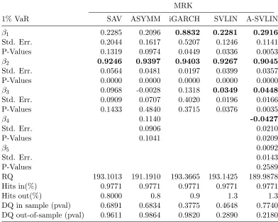
Table 2.1 Comparison of CAViaR, SVLIN models for MRK at 1% VaR . . . 29
Table 2.2 Comparison of CAViaR, SVLIN models for MRK at 5% VaR . . . 30
Table 2.3 Comparison of CAViaR, SVLIN models for MER at 1% VaR . . . 31
Table 2.4 Comparison of CAViaR, SVLIN models for MER at 5% VaR . . . 32
Table 2.5 Comparison of CAViaR, SVLIN models for MDT at 1% VaR . . . 33
Table 2.6 Comparison of CAViaR, SVLIN models for MDT at 5% VaR . . . 34
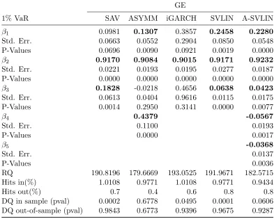
Table 2.7 Comparison of CAViaR, SVLIN models for GE at 1% VaR . . . 35
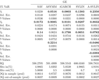
Table 2.8 Comparison of CAViaR, SVLIN models for GE at 5% VaR . . . 36
Table 2.9 Comparison of CAViaR, SVLIN models for F at 1% VaR . . . 37
Table 2.10 Comparison of CAViaR, SVLIN models for F at 5% VaR . . . 38
Table 2.11 Comparison of CAViaR, SVLIN models for DNA at 1% VaR . . . 39
Table 2.12 Comparison of CAViaR, SVLIN models for DNA at 5% VaR . . . 40
Table 2.13 Summary Statistics of the log returns and coefficient of variation of the estimated volatilities . . . 42
Table 2.14 SV parameter values used in simulation . . . 42
Table 2.15 Comparison of the CAViaR, SVLIN models for θ1 at 5% VaR undert1, t2, and N(0,1) error distributional assumptions . . . 44
Table 2.16 Comparison of the CAViaR, SVLIN models for θ2 at 5% VaR undert1, t2, and N(0,1) error distributional assumptions . . . 45
Table 2.17 Comparison of the CAViaR, SVLIN models for θ3 at 5% VaR undert1, t2, and N(0,1) error distributional assumptions . . . 46
Table 2.19 Comparison of the CAViaR, SVLIN models for θ5 at 1% VaR undert1, t2,
and N(0,1) error distributional assumptions . . . 48 Table 2.20 Comparison of the CAViaR, SVLIN models for θ6 at 1% VaR undert1, t2,
and N(0,1) error distributional assumptions . . . 49 Table 2.21 Comparison of the out of sample test results of the 5% VaR estimates
ob-tained for the best CAViaR model, SVLIN, and benchmark . . . 50
Table 2.22 Comparison of the out of sample test results of the 1% VaR estimates ob-tained for the best CAViaR model, SVLIN, and benchmark . . . 51
Table 3.1 Comparison of EMM and RQMM estimates for nonnormal distributions un-der local misspecification . . . 72
Table 3.2 Comparison of RQMM and EMM estimates under correct model specification under normality with moderate sample sizes . . . 76
Table 3.3 Comparison of RQMM and EMM estimates under correct model specification under normality with small sample sizes . . . 78
Table 3.4 Comparison of Bias, MSE for competing Auxiliary models under RQMM with incorrect specification. . . 80
Table 4.1 Comparison of the out of sample test results of the 5% and 1% VaR estimates obtained from RQ-KF for GE, F, DNA and MER . . . 87
Table 4.2 Comparison of RQ-KF and QML estimates for standard normal, t5 and t2
distributions . . . 90
Table 4.3 Comparison of the out-of-sample test results of the 5% VaR estimates ob-tained from the RQ-KF method. . . 91
LIST OF FIGURES
Figure 2.1 Log returns of 6 stocks . . . 28
Figure 3.1 Frequency Density plot ofα1 estimated by RQMM and EMM (dash-dot red
line) whenθ= [−0.7,0.9,0.363],ǫt∼t1, T=500, and 500 MC runs. . . 71
Figure 3.2 Frequency Density plot ofα1 estimated by RQMM and EMM (dash-dot red
line) whenθ= [−0.7,0.9,0.363],ǫt∼CO, T=500, and 500 MC runs. . . 73 Figure 3.3 Frequency Density plot ofα1 estimated by RQMM and EMM (dash-dot red
line) whenθ= [−0.7,0.9,0.363],ǫt∼t2, T=500, and 500 MC runs. . . 73
Figure 3.4 Frequency Density plot ofα1 estimated by RQMM and EMM (dash-dot red
line) whenθ= [−0.7,0.9,0.363],ǫt∼t3,T=500, and 500 MC runs. . . 74
Figure 3.5 Frequency Density plot ofα1 estimated by RQMM and EMM (dash-dot red
line) whenθ= [−0.7,0.9,0.363],ǫt∼CN, T=500, and 500 MC runs. . . 74 Figure 3.6 Frequency Density plot ofα1 estimated by RQMM and EMM (dash-dot red
line) whenθ= [−0.7,0.9,0.363],ǫt∼Cauchy(0, 0.5), T=500, and 500 MC runs. . 75 Figure 3.7 Frequency Density plot ofα1 estimated by RQMM and EMM (dash-dot red
line) whenθ= [−0.7,0.9,0.363],ǫt∼Cauchy(0, 1.5), T=500, and 500 MC runs. . 75 Figure 3.8 Frequency Density plot ofα1 estimated by RQMM and EMM (dash-dot red
line) whenθ= [−0.7,0.9,0.363],ǫt∼Cauchy(0, 2), T=500, and 500 MC runs. . . . 76 Figure 3.9 Frequency Density plot ofα1 estimated by RQMM and EMM (dash-dot red
line) whenθ= [−0.7,0.9,0.363],ǫt∼N(0,1), T=1000, and 500 MC runs. . . 77 Figure 3.10 Frequency Density plot ofα1 estimated by RQMM and EMM (dash-dot red
line) whenθ= [−0.7,0.9,0.363],ǫt∼N(0,1), T=500, and 500 MC runs. . . 77 Figure 3.11 Frequency Density plot ofα1 estimated by RQMM and EMM (dash-dot red
line) whenθ= [−0.7,0.9,0.363],ǫt∼N(0,1), T=50, and 500 MC runs. . . 79 Figure 3.12 Frequency Density plot ofα1 estimated by RQMM and EMM (dash-dot red
Figure 3.13 Frequency Density plot ofα1 estimated by RQMM and EMM (dash-dot red
line) whenθ= [−0.7,0.9,0.363],ǫt∼N(0,1), T=200, and 500 MC runs. . . 81
Figure 4.1 5% and 1% VaR estimates for the short positions and their corresponding log returns for GE, F, DNA and MER. . . 88
Figure 4.2 Comparison of frequency density plots of α1 obtained from RQ-KF and
QML methods. . . 92
Figure 4.3 Comparison of Box plots of ˆσv obtained from RQ-KF and QML methods . 93
Figure 5.1 Comparison of estimated conditional return probabilities calculated by Watan-abe’s method and those computed using the Gram-Charlier representation . . . 102
Figure 5.2 Comparison ofP(yt|yt−1) calculated by Watanabe’s method and that com-puted using the Gram-Charlier representation for θ=(0.7,0.5,0.98). . . 103 Figure 5.3 Comparison of estimated conditional return probabilities calculated by
Watan-abe’s method and those computed using the Gram-Charlier representation for CF application . . . 103
Chapter 1
Introduction
In mathematical finance and financial statistics, the Stochastic Volatility (SV)
model is used widely for modeling the time-varying volatility in financial markets. The
development of the model and methodology related to its usage and growth is driven by a
need for better pricing of options, efficient asset allocation and risk assessment. The scope
of study in this thesis is related to risk assessment by calculating Value at Risk (VaR) and
robust estimation using Quantile Regression (QR) techniques, when the underlying process
is SV.
1.1
Motivation
A crucial aspect of measuring VaR is the volatility of the data. Hence, selecting
a volatility model that fits the data appropriately, and its applicability, are important
con-siderations in achieving the goal of VaR computation. In existing VaR methodology, much
of the interest is concentrated towards the ARCH group of models introduced by Engle
(1982), due to its deterministic nature of volatility and easier applicability. Relatively, the
SV group of models are not as preferred, due to the volatility formulated as a stochastic
process. With the emergence of high frequency data, SV models have again taken
cen-terstage in econometric analysis, risk management and asset allocation. In pricing theory,
continuous SV models have always formed the core of research. Hence, SV models form an
attractive modeling tool with tremendous scope in multiple research arenas in finance.
An important feature of the SV models is that the volatility has its own stochastic
process. This results in difficulties in the direct calculation of the likelihood and VaR
estimation of SV models. In the 1990s, several computationally intensive methods were
Computation based methods such as Bayesian Monte Carlo (Jacquieret al., 1994),
Simulated Maximum Likelihood (SML) (Danielsson, 1994) and Simulated Method of
Mo-ments (SMM) (Duffie and Singleton, 1993), (Gourieroux et al., 1993) methods produce
better results in terms of accuracy and efficiency than the less computationally
inten-sive tools such as Quasi Maximum Likelihood (QML) developed by Nelson (1988), Harvey
et al.(1993), Ruiz (1994), Method of Moments (MM) technique (Taylor, 1986), Generalized
Method of Moments (GMM) (Melino and Turnbull, 1990), (Andersen and Sørensen, 1996).
Monte Carlo evidence suggests that MM, GMM, QML techniques suffer from poor small
sample performance. Watanabe (1999)’s nonlinear filtering maximum likelihood (NFML)
method provides a balance in that it gives good results in small samples without being as
computationally demanding as a simulation based approach. Each of the aforementioned
methods have their own set of advantages and we were motivated to study some of these
methods (viz., QML, NFML, and EMM forming the basis for RQ-KF, NF scheme, RQMM
methods, respectively) in the context of VaR calculation.
Calculation of VaR entails the knowledge of one-step ahead predictive densities.
However, in the SV approach, the one step ahead densities cannot be obtained directly.
Watanabe (1999) uses the QML estimates as a starting point for his nonlinear filtering
(NF) method. The NF technique is an improvement over QML. Instead of using the first
two moments as in the standard Kalman approach in QML, it uses the conditional densities
directly in its filter to calculate the likelihood; hence, the conditional VaR’s can be obtained
subsequently. NF is based on a scheme that depends on a series of conditional integrals,
where the integrals are evaluated numerically using piecewise linear approximations to the
density function, motivated by Kitagawa (1987)’s work. One of the important considerations
here is the choice of the number and location of the nodes that would suffice for a good
approximation without compromising on computational demands. Appropriate nodes are
chosen according to an approach suggested by Tanizaki (1996). The method computes
the one-step ahead predictive densities as part of the algorithm. Hence, they can be used
for likelihood computation (denoted by nonlinear filtering maximum likelihood (NFML))
and also as a filtering process for VaRs. NF’s filtering method does not depend on the
state space representation of the model, hence various extensions of the SV models can
be easily tackled. Also, as long as known parametric forms of the volatility process and
their relationship with their returns can be modeled, NF scheme finds ready application.
excellent groundwork for VaR calculation.
The Conditional Autoregressive Value at Risk (CAViaR) model (Engle and
Man-ganelli, 2004) moves the focus of attention from the conditional distribution of returns
directly to the behavior of the quantiles. The evolution of quantile over time is specified
using an autoregressive quantile framework; hence the RQ objective criterion developed by
Koenker and Bassett (1978) can be adapted for estimation. The Quantile Regression (QR)
estimator is increasingly becoming an important tool for analysis, which helps in fitting
parsimonious models in lieu of full conditional distributions. Another important aspect is
that the method produces robust statistics and hence it finds its application in financial
data scenarios with fat tailed distributions, and data with outliers. In applications, a robust
inferential technique often proves to be beneficial in the case of misspecified models.
The motivation behind the methodologies proposed in this dissertation came from
the CAViaR approach proposed by Engle and Manganelli (2004), based on the regression
quantile framework introduced by Koenker and Bassett (1978). The CAViaR group of
models provide a general framework for estimation of conditional VaRs. Some of their
proposed models are derived from the popular autoregressive conditional heteroscedastic
models. In ARCH type models, conditional quantiles are directly linked to the standard
deviation of the distribution. Hence, an extension and application of their work in the SV
context provides a strong motivation. This technique is particularly interesting because the
likelihood computation in SV is circumvented which in itself involves an equally challenging
problem.
The primary focus of research earlier was to efficiently and accurately estimate
the SV parameters and volatility. However, consideration of heavy tailed distributions,
and misspecification in models form an important premise in present day research. High
kurtosis is endemic to financial data. We use this assumption heavily in our research.
Asai (2008) compares an Asymmetric Stochastic Volatility (ASV) model withtdistribution innovations with the multifactor SV (MFSV) model. Results using returns on the S&P
500 Composite and Tokyo stock price indexes and the Japan-US exchange rate indicate
that the ASV-t model provides a better fit than the MFSV model on the basis of Akaike information criterion (AIC) and the Bayes information criterion (BIC). Several researchers,
including Liesenfeld and Jung (2000), Watanabe and Asai (2003), show using a heavy tailed
distribution for the error provide a better means in describing the high kurtosis in the data.
SV parameters and VaR calculation.
The efficient method of moments (EMM) technique (Bansal et al.(1993), Bansal
et al. (1995), Gallant and Tauchen (1996)) is a flexible tool used for estimation. EMM is a
culmination of the efficiency provided by the maximum likelihood (ML) approach coupled
with the flexibility and affordability of the GMM. EMM is used where the ML method
is infeasible or computationally intensive. Therefore, it finds its application directly in
the SV context. The method employs an auxiliary data model that approximates the
salient features of the true data generating process and has a readily computable likelihood
function, in a closed form. The score equations of the auxiliary model are used as the
moment equations to attain the efficiency of the ML asymptotically. The EMM as a method
has its origins linked to the Indirect Inference (II), and Simulated Method of Moments
(SMM) techniques.
The flexibility of the approach serves as the motivation behind our Regression
Quantile Method of Moments (RQMM) methodology. It provides a general framework so
that later developments can be incorporated easily. We use SV model as the benchmark
throughout. The results obtained from our methodologies can be extended to the other
situations like Asymmetric SV (ASV) models, Hermite Stochastic Volatility (HSV) models
accounting for leverage effects, heavy-tailedness etc.
This dissertation addresses both robust statistical estimation and VaR calculation
in a unified approach. Conditional quantiles or VaRs are related to the conditional
dis-tributions of the process. The Quantile Regression (QR) estimation is an important tool
for analysis in fitting parsimonious quantile models in lieu of full conditional distributions.
We propose two methods (i) Regression Quantile Method of Moments (RQMM) and (ii)
Regression Quantile - Kalman Filtering method (RQ-KF) based on the QR approach that
can be used for estimation of the SV model as well as for VaR calculation. The RQMM is a
simulation-based indirect inference procedure where recursive quantile models are used as
the auxiliary models, with the gradients of the RQ objective function (also known as the
check or tick function) serving as the basis for estimating equations. This was motivated
by the EMM approach used in SV model estimation and the CAViaR method proposed by
Engle and Manganelli (2004). The check criterion gradient serves as a replacement of the
score equations in EMM. The main concern is to develop robust statistics; therefore
appli-cation of the check function as a nonparametric, flexible criterion provides a solution. Since
the iGARCH are reasonable choices. Hence, when the optimum parameter estimates for
SV are attained, given that the auxiliary model approximates the true data model well,
the estimated conditional quantiles will closely approximate the conditional quantiles of the
SV, while also providing estimates for the SV model parameters. Details are provided in
Chapter 3.
As an extension of CAViaR models, optimal linear quantile models (SVLIN and
Asymmetric-SVLIN) based on the underlying SV assumption is derived. This is used along
with the other CAViaR specifications as auxiliary models. The RQ-KF is a computationally
simple procedure combining the good properties of QML and QR methodologies. The first
step requires obtaining initial estimates using QML. Using a recursive model motivated by
SV, quantile estimates are produced by the Kalman Filtering scheme based on the initial
parameter estimates. These quantiles are then plugged into the check function to yield
robust estimates. Details are provided in Chapter 4.
Financial data are known to exhibit heavy-tailedness characteristics. With
sim-ulation studies, these tools are shown to be stable in the presence of heavy-tailedness in
the data. Comparison of the RQMM method with the EMM under different data scenarios
show that RQMM is stable under local misspecification, and heavy-tailedness. Comparison
of the RQ-KF method with the existing QML method provide competitive results in terms
of model estimation. Also, risk evaluation test results show desirable statistical properties
of the quantile estimates obtained from these methods. Applications to real data and
sim-ulation studies on different parameter settings of the SV model provide empirical support
in favor of the quantile model specifications including the CAViaR, SVLIN and A-SVLIN.
Calculating the likelihood in SV model requires integration over an infinite
dimen-sional state vector. Using Hermite polynomial approximations, we find an alternative finite
dimensional approximation to the infinite dimensional state vector. We propose a Gram
Charlier density approximation for the conditional predictive volatility density given past
returns to compute the one step ahead predictive return densities in the existing Nonlinear
Filtering (NF) scheme proposed by Watanabe (1999), Fridman and Harris (1998). Our
method requires a reduced number of node points based on the coefficients of the Hermite
polynomial, when compared to the earlier propositions. With this approximation, the
con-ditional density calculated can be used in the likelihood function for SV parameters as part
of the estimation process, or to find the conditional quantile for estimated parameters as
state vector for evaluating with this approach is provided. The proposed algorithm can
be used as a substitute for other numerical integration approximations based on choosing
appropriate node points (see Watanabe (1999), Fridman and Harris (1998)).
Most of the earlier work for SV model estimation was coupled with obtaining a
smoothed estimate of the volatility process by a nonlinear filter. In the Bayesian case of
Jacquieret al. (1994) the smoothed estimates are obtained as a by-product of the method.
In the non-Bayesian cases of MM and QML, standard approximate Kalman filtering schemes
are used. Also, a quantile forecast in practice, is a two-step approach: model used to forecast
volatility followed by a method of computing quantiles from volatility forecasts. Both our
methodologies are aimed at parameter estimation and computing quantiles directly.
1.2
Outline of thesis
In Chapter 2, we give a brief overview of VaR and the existing methods for VaR
calculation and evaluation. CAViaR model estimation by Regression quantiles is outlined
briefly. We propose two linear quantile specifications based on the underlying assumption
of SV. We compare the performance of these two models with the CAViaR models by using
a real data analysis based on six stocks, and simulation studies based on several parameter
settings of the SV model. The NF scheme is used as a benchmark to provide VaR estimates.
In Chapter 3, we provide a brief summary of EMM as our motivation. Next, we
propose the RQMM methodology, followed by a discussion on the asymptotic properties of
its estimates. We compare the performance of the RQMM with EMM under several
heavy-tailed distributional assumptions, and misspecification with a simulation study. Under
correct specification, the efficiency of RQMM estimates with EMM are also compared. It
is to be noted that the VaR estimates using this method are reflective of our findings in
Chapter 2. This is followed by a discussion.
In Chapter 4, we propose the RQ-KF method. We compare the performance of
the method with QML with the help of a simulation study followed by a discussion.
In Chapter 5, we develop an algorithm based on the GC representation of the
predicted conditional volatility density given the past returns. The incorporation of this
scheme to the existing NF scheme is discussed. The application of such a scheme with
respect to model estimation and VaR calculation is validated by a data exercise.
Chapter 6 summarizes the findings of the methods in Chapter 2–5 and discusses
The remaining part of this chapter provides an overview of the volatility models.
1.3
Volatility models
1.3.1 SV models
The volatility of a financial asset is the standard deviation per unit time of the
returns of an asset. In financial markets, volatility is a predominant feature, hence it plays a
very important role in the determination of risk and valuation of options and derivatives. In
financial terminology, volatility is the standard deviation and is directly related to the risk
associated with holding financial securities, portfolio choice and investment decisions. The
link between finance and Brownian motion goes way back till Bachelier (1900) who proposed
a model for the French stock prices. A natural extension of a more reasonable model
was proposed by Osborne (1959) where the price followed an exponential (or geometric)
Brownian motion. The standard model that describes the behavior of the price process
P(t) is the solution of the stochastic differential equation (SDE) given by (1.1). Let us denote byP(t) the continuous time process and let Ptdenote its discrete analogue.
dP(t) =P(t)(µdt+σdZ1(t)) (1.1)
where t is measured in units of one year, Z1(t) is a Brownian motion while the mean, µ
and volatility, σ, are constant parameters of the model. The time convention is chosen to ensure thatσ can be interpreted as an annualized volatility. This SDE has solution
P(t) =P(0) exp{σZ1(t) + (µ−
1 2σ
2)t}. (1.2)
The discrete time analogue of (1.1) based on a daily sequence of observations (Pt)t≥0 is
lnPt−lnPt−1≡∆(lnPt) =ν+σZt (1.3)
where (Zt) is a sequence of independent normal random variables with zero mean and variance 1/250 (number of business days per year).
Stochastic volatility models are useful because they try to incorporate the empirical
observation that volatility appears to be stochastic. The SV candidate models have been
motivated by intuition, convenience and tractability and some of them have been listed
in equations (1.4), (1.5), (1.6), (1.7), and (1.8). Scott (1987), Wiggins (1987), Hull and
proposed models of the form
dP(t)
P(t) =σ(t)dZ1(t) +µdt (1.4) whereσ(t), the SV process is itself the solution of a stochastic differential equation. It is to be noted that in each of the cases enumerated hereunder,Z2 is a Brownian motion perhaps
correlated with the Brownian motionZ1 which forms part of the specification of (1.4). Let
us denote the correlation byρsuch thatE(dZ1(t)dZ2(t)) =ρdt. Further, we assume that ρ
is a constant with modulus less than one.
dσ(t) =σ(t)(α0dt+γdZ2(t)) (1.5)
The first model given by (1.5) was introduced by Hull and White (1987) with ρ = 0 and Wiggins (1987) considered the general case. Here the logarithm of the volatility is a drifting
Brownian motion. Scott (1987) considered the model (1.6) where the logarithm of the
volatility is an Ornstein-Uhlenbeck (OU) process, and the discrete time analogue of the OU
process is an AR(1) time series. The discrete version of this model is referred to as the SV
model in the thesis, and we focus our work on this model. These models (1.5) and (1.6)
have been formulated such that the volatility is positive.
dlnσ2(t) =α1(α0−lnσ2(t))dt+γdZ2(t) (1.6)
The model given below (1.7) was introduced by Scott (1987) and further investigated by
Stein and Stein (1991) keeping ρ = 0. In this case, the volatility process itself is the OU process. However, the disadvantage of this model is that the volatility could easily become
negative but (1.4) remains well defined.
dσ(t) =α1(α0−σ(t))dt+γdZ2(t) (1.7)
In 1988, Hull and White (1988) proposed a model and Heston (1993) investigated further
with the general case ofρ6= 0 of the form
dσ(t)2 = (α0−α1σ(t)2)dt+γσtdZ2(t) (1.8)
Two other models of note were proposed by Johnson and Shanno (1987) who modeled both
the price and the volatility processes as constant elasticity of variance (CEV) processes (1.9)
(1.9) and the logarithm of volatility to be an OU process. The CEV model proposed by
Cox and Ross (1976) is
dP(t)
P(t) =σ(P)dZ1(t) +µdt (1.9) whereσ(P) =σPα−1 andα∈(0,1). In CEV models, the price and volatility are negatively correlated.
Even though continuous time models provide the natural framework for analysis
of option pricing, discrete time models are required for the statistical analysis for the
cal-culation of VaR. The discrete time data models can be seen as a skeleton of the continuous
time process. In the literature, the discretized version of the SV models have been termed
as Stochastic variance models, autoregressive variance model etc., but in our discussion the
SV model would mean the discretized SV model (1.6) (henceforth). In SV models, the
logarithm of volatility is modeled as an AR(1) process with white noise. However, due to
its non-deterministic nature, evaluation of the exact likelihood is challenging, hence they do
not share the same popularity as the ARCH, GARCH models and have limited empirical
applications.
In this dissertation, we use the SV model as defined in (1.10) below. Letytbe the stochastic process of returns
yt=σtǫt ǫt∼N(0,1) (1.10)
whereσ2
t is the conditional variance of theyt. In the simplest SV model framework, the log of squared volatility is expressed as an AR model:
ln(σ2t) =α0+α1ln(σ2t−1) +vt vt∼N(0, σ2v)
whereǫt andvtare assumed to be independent of each other. The parameters of the model are denoted by θ={α0, α1, σv2}.
Harvey and Shephard (1996) considered the leverage effect and introduced the
Asymmetric Stochastic Volatility (ASV) model where an addition Corr(ǫt,vt+1) = ρ was
made to the SV model.
The Hermite SV (HSV) models were proposed by Meddahi (2001). This is a
novel approach of modeling volatility in discrete and continuous time. The distinguishing
feature in this model is that the variance is a linear combination of the Hermite polynomial
are governed by the dynamics of the state variables. This state variable may be governed
by a Gaussian AR(1). It is important to note that the specification of the variance function
based on the linear combination of the Hermite polynomials of state variable is a flexible
model. Hence, the HSV model is formulated to keep the higher polynomial weights as free
parameters that need to be estimated.
yt = σtǫt ǫt∼N(0,1) σ2t = a0+a2(ft2−1)
ft = βft−1+ p
1−β2v
t vt∼N(0,1)
where θ = (a0, a2, β) are the parameters. The HSV models successfully generate fat tails
for the variance and return processes.
For an overview of SV models, see Shephard (2005).
There are two main classes of discrete time models for stock prices with volatility.
The first class, stochastic volatility models, is a discrete time approximation to the
contin-uous time SV models that we outlined above. The second class constitutes the conditional
heteroscedastic models.
1.3.2 Conditional Heteroscedastic models
The autoregressive conditional heteroscedastic (ARCH) model introduced by Engle
(1982) is a pioneering work that led to the systematic development of a series of contributions
that falls into the category of conditional heteroscedastic models. The econometric literature
is replete with many models that are being used to quantify the uncertainty in future
instantaneous volatility models. An ARCH (m) model is
at = σtǫt
σt2 = α0+α1at−12+. . .+αmat−m2
whereatis the mean corrected, serially uncorrelated asset return andǫtis a sequence of i.i.d. random variables with mean 0 and variance 1. Another widely popular model that capture
the dynamics of the volatility process is the GARCH structure given in (1.11). Bollerslev
(1986)’s GARCH model is given by
σ2t =α0+
m
X
i=1
αia2t−i+ s
X
j=1
whereat=yt−µtis the mean corrected log return. Other extensions of the aforementioned models were made viz. EGARCH (Nelson, 1991) to capture asymmetry, and CHARMA
(Tsay, 1987) which uses random coefficients to produce conditional heteroscedasticity.
AR-MACH(1,1) (Taylor, 1986) model is given by (1.12):
σt=α0+α1|at−1|+β1σt−1 (1.12)
EGARCH(m,s) (Nelson, 1991) model, shown in (1.13) is as follows:
lnσ2t =α0(1−α1−α2−. . .−αm)+
+α1lnσ2t−1+α2lnσt2−2+. . .+αmlnσ2t−m+ +g(ǫt−1) +β1g(ǫt−2) +. . .+βs−1g(ǫt−s)
(1.13)
g(ǫt) =δǫt+γ[|ǫt| −E(|ǫt|)]
whereδ andγ are real constants and the coefficients (δ+γ) and (δ−γ) show the asymmetry in response to the positive and negative values.
The GARCH model is a widely used tool to model financial data. Its strength lies
in capturing volatility clustering of large price movements. The models described in this
section are popular approaches to describe the changing volatility. The variance,σ2
t, of the current return is written in terms of a nonstochastic function of the past observations. One
of the many attractions of using such models is that the deterministic nature of the variance
process leads to an exact likelihood, making estimation and forecasting straightforward.
Kimet al.(1998) provide evidence of better in-sample-fit of the SV model relative
to GARCH-type models. Because of their well documented advantage in the literature,
there is a need to develop and study methods that produce conditional quantile estimates,
under the SV framework.
The next chapter gives a brief overview of the different methodologies used for
Value at Risk calculation. The CAViaR model is discussed next followed by a proposition for
SVLIN and ASVLIN models. These quantile specifications are derived from the relationship
to the linear predictor of the latent volatility process under SV. Analysis of these models
in the context of VaR performance are carried out with quantiles obtained from the NF
Chapter 2
VaR Estimation
With rising emphasis on risk management, portfolios are marked to market daily.
The fluctuations intrinsic in the data captured, for instance, by volatility, play a very
important role in VaR calculation. The two broad classes of modeling heteroscedasticity in
financial data viz. stochastic volatility models and the ARCH group of models, provide a
well established framework for VaR computation. Conditional heteroscedastic models such
as ARCH, GARCH, EGARCH and others are often used to model volatility clustering,
leverage effects etc. in the data. Stochastic volatility model is another widely used model
with a wide application in finance. We focus this study on SV models. Due to the latent
volatility modeled as a stochastic process, direct VaR computation is not straightforward.
The CAViaR group of models, proposed by Engle and Manganelli (2004), provides
an unique way to directly estimate the conditional quantiles of interest, ie. Value at risk.
This is achieved by minimizing the Regression Quantile (RQ) criterion, a robust loss function
for a group of models based on conditional quantiles regression motivated by characteristics
of financial data dynamics. Although the quantile specifications discussed under CAViaR,
are motivated by the ARCH group especially, however, they can be applied more generally.
Within this setup, we are interested in seeking a quantile model motivated by the SV model.
We call this the SVLIN model. We further seek a quantile specification under the ASV model
and name it the A-SVLIN model. With data generated from SV model, we evaluate the
performance of the CAViaR models with the SVLIN model. The RQ criterion, devoid of
any distributional assumptions, is used to gauge results in heavy-tailed error distribution
situations, suitable for financial data. As a benchmark, we obtain the VaRs’ directly from
the Dynamic Quantile test (proposed by Engle and Manganelli (2004) and Chernozhukov
(1999) independently) and other tests from the extant literature.
Section 2.2 gives a brief account of the existing methods followed by a description
of the CAViaR method in the next section. Sections 2.4 and 2.5 discusses the RQ objective
criterion introduced by Koenker and Bassett (1978), and tests for VAR evaluation,
respec-tively. The SVLIN and A-SVLIN models are based on obtaining the best linear predictor
using the Kalman filter for SV models and ASV models respectively, discussed in Section
2.6. The VaR computed from Watanabe (1999)’s method as benchmark is described in the
Section 2.7. Results from the empirical study based on both application to stock data and a
simulation study are presented in Section 2.8. The interpretation and results are discussed
in Section 2.9.
2.1
Value at Risk
Value at Risk (VaR) is used as a standard measure for evaluating risk in
finan-cial institutions and organizations. It was introduced after the finanfinan-cial disasters of the
1990’s. Although it started out as a tool to measure and monitor market risk, its usage
has increased tremendously in the past few years to several other types of risk, eg, credit
risk, liquidity risk, operational risk and subsequently to an integrated enterprise-wide risk.
With globalization of financial markets leading to multiple sources of risk, pressure from
regulators, and technological advances, its generalizability and implicit summarization of
the risk scenario have led to its indispensable application to firm-wide risk management.
Also, the boundaries between the abovementioned risks are becoming blurred. Hence, it
provides an aggregate viewpoint for measuring a portfolio’s risk. Its use is not only confined
to derivatives but to all financial instruments. It provides an easy-to-use benchmark
mea-sure of risk, adopted by regulators (Basel committee on Banking supervision, U.S. Federal
reserve, etc.), institutions with an exposure to financial risk, risk managers alike.
In recent years there has been an ever increasing demand to measure risk, and
effective methods that can evaluate such critical situations are limited. The calculation of
VaR has to be intrinsically related to the real world data scenarios. Dynamic models that
closely replicate characteristics of financial data such as heavy tailedness, volatility
cluster-ing, and skewness have become relevant. In order to capture the time varying volatility, SV
models are often used, in which the conditional variance is specified to follow a latent
processes define the volatility equation. Their discrete counterparts are used to develop
statistical methodologies for VaR calculation. Since VaR (or, quantiles) are directly related
to the volatility process, they are tightly linked, and share similar characteristics. Due to
the random component in the SV volatility equation, likelihood based model estimation,
in itself poses a challenging problem, and so does VaR computation. They nevertheless
provide a very attractive alternative to time varying conditional variance modeling, and it
is of interest to study methods that compute VaR under this modeling framework.
Engle and Manganelli (2004) proposed autoregressive models for the VaRs,
es-timating the parameters by minimizing the Regression Quantile criterion (Koenker and
Bassett, 1978). Four models were proposed which can be seen as extensions to the widely
used conditional heteroscedasticity (ARCH) models (Bollerslev, 1986).
A natural extension to their work is to implement a similar objective of finding
conditional VaR calculation methods in a regression setup, under the SV model framework.
This proposition is especially attractive in the context of SV since this technique circumvents
the likelihood calculation and directly yields VaR estimates. Also, their performance in
the context of heavy tailed distributions should also be considered, since financial data
exhibits high kurtosis. The empirical study in Section 2.8 verifies that the proposed model
successfully describes the evolution of quantiles at the tails, especially, in cases of SV models
with heavy tailed error distributions.
Let us denote ∆Vt,l=Pt+l−Ptas the change in the value of the financial position from timet tot+l, where Pt is the price process andFl(x) is the cumulative distribution function (cdf) of ∆Vt,l. −VaRt(τ, l) can be defined as the loss faced by a financial position during a given time period (t, t+l) for a given confidence level τ under normal market conditions. We can formally define VaR of a long position over a time horizon l with probability τ as
τ = Pr[∆Vt,l ≤ −VaRt(τ, l)] =Fl(−VaRt(τ,l))
where the VaR, −VaRt(τ, l) is a negative value (loss), by the above notation. Following convention, VaRt is a positive value measured in the currency of interest and τ is the
confidence level. Hence we would look at the entire quantity−VaRt as Value at Risk (VaR)
the log returns. Let us denote the log returns by
yt= ln Pt Pt−1
Hence a negative yt means loss. Modeling and estimation is usually carried out by using log returns because they have been shown to exhibit the properties of volatility clustering,
stationarity, possessing almost zero autocorrelation, conditional heteroscedasticity. Hence,
a VaR definition needs to be formalized with respect to the returns. Following the notation
of Engle and Manganelli (2004), let {yt}Tt=1 be the time series of portfolio returns. VaR at
a time tis given by
P r[yt<−VaRt|Ωt−1] =τ
where Ωt−1 denotes the information set at the end of time t−1. Analyzing the left or
the right tail of the c.d.f. depends on whether you are a holder of the long position or a
short position respectively. The above definition is applied by the holder of a long position
because he faces a loss when the value of the portfolio decreases. However, a change in the
sign of the variable would make the holder of a short position study the left tail as well.
Hence, it suffices to use this definition for the following discussion.
Some of the prevalent statistical methodologies frequently used in evaluating VaR
can be broadly categorized into the
following:-Econometric approaches (EA),quantile regression(QR),extreme value distributions (EVD)
and historical simulation (HS). RiskM etricsT M, proposed by J.P. Morgan, is a particular
case of EA and is a widely used tool. For an overview of VaR, see Jorion (2007). The next
section sketches a brief review of these methods followed by an outline of the rest of the
paper.
2.2
Existing Methods of VaR Estimation
J. P. Morgan developed RiskM etricsT M methodology for VaR calculation. For a better exposition, the reader is referred to Logerstaey and More (1995). This method
assumes that the continuously compounded daily return of a portfolio follows a conditional
normal distribution. RiskMetrics assume that yt|Ωt−1 ∼N(µt, σt2), where µt is the condi-tional mean and σt2 is the conditional variance of yt. In addition, it also assumes that the two quantities evolve over time following the simple model:
Hence, it assumes that the daily log returns satisfyingyt=σtεtis an IGARCH(1,1) process without a drift. For such a random-walk IGARCH model, the conditional distribution of
a multiperiod return is easily available. Specifically, for a k-period horizon the conditional
distributionyt[k]|Ωt isN(0, σt2[k]), where
yt[k] = t+k
X
i=t+1
yi
and σ2t[k] can be shown to be equal to kσt2+1. Therefore, for a k-period horizon, it follows thatV aR(k) =p(k)×V aR.
There are several econometric models for the mean and the volatility processes.
To show an example, for a general time series model for yt let us use the ARMA, GARCH to model the mean and the volatility processes respectively.
yt=φ0+
a
X
i=1
φiyt−i+at− b
X
j=1
θjat−j
at=σtǫt σ2t =α0+
u
X
i=1
αia2t−i+ v
X
j=1
βjσ2t−j
where at is the mean corrected, serially uncorrelated asset return and ǫt is a sequence of i.i.d. random variates with mean 0 and variance 1. The residuals may be assumed to follow
a known parametric distribution (e.g., Normal, t etc.). Other conditional heteroscedastic models viz. IGARCH, GARCH-M, EGARCH, CHARMA, etc. can also be used to model
the volatility process. Hence, quantiles from these conditional distributions can be evaluated
accordingly. This method is relatively simple to use.
Quantile regression is a nonparametric approach to VaR computation. It is more
appropriate to include the covariate information while estimating the quantiles for the
conditional distributions. Hence, in this case, Ωt−1 introduced earlier which represent the
information till the end of period t−1 contains further information on the covariates. Koenker and Bassett (1978) developed the quantile regression theory by formulating the
sample quantile problem to a linear regression one. One of the recent papers using the
regression quantile method is the CAViaR model proposed by Engle and Manganelli (2004).
They propose an autoregression of the conditional VaRs’ and their approach is discussed in
The generalized extreme value distribution (EVD) of Jenkinson (1955)
encom-passes the three types of limiting distribution of Gnedenko (1943). Since we are interested
in the extreme tail of the distribution for the computation of VaR and because the EVD
is appropriate for analyzing extreme events, EVD theory is often used in VaR calculations.
The idea is to partition the sample of the returns into nonoverlapping subintervals. Using
the minimum values from these subintervals, we estimate the EVD parameters.
Estima-tion of the three parameters in the EVD can be carried out parametrically by maximum
likelihood or by minimizing the sum of squared errors in a regression setup, or
nonparamet-rically. Once the distribution is known, VaRs can be calculated. This method depends on
the choice of the subintervals for a given data set. Hence, in order to make the minimum
among the subinterval points appreciably close to the real extreme data, sufficient data are
required.
A common method for VaR estimation is historical simulation (HS), in which the
simulated distribution of returns is simply the empirical distribution of the past
observa-tions. The advantage of this method is that it makes no distributional assumptions, that it
is nonparametric. If historical data has been collected in-house, the same data can be used
for VaR calculation. It is relatively easy to implement; however, it has major drawbacks.
The method applies equal weight to its past observations. Since it considers only one
real-ization of the data, in cases of large deviations of the data from the true distribution, the
quantiles obtained by HS can be greatly affected. Moreover, it is slow to capture structural
breaks that can be easily detected by, for instance, Riskmetrics. The choice of sample size
can also have a huge effect on the predicted values. Some variations have been proposed
in the literature to overcome some of these disadvantages. For example, Boudoukh et al.
(1998) proposed a method which applies exponentially declining weights to the past returns.
Although its conceptual simplicity has attracted a wide range of users, the
com-putation of VaR is a challenging statistical problem and most of the methods developed so
far are based on simplifying assumptions. Standard model free methods such as historical
simulations, rely on a single sample path and does not require any distributional
assump-tions. Reliable risk measurement requires to account for the characteristics of returns data
like negative skewness and leptokurtosis. Models with a time varying conditional volatility
structure are often used, but the usual choice of error distributions may not consider the
excess kurtosis present. We need to add more methods to the available toolkit for VaR
the standard deviation behavior, if the volatility modeling is based on a flexible structure,
consequently, the flexibility will lend itself to quantile model behavior as well. Hence, a
quantile regression based on the SV framework can lead us to a good model that captures
the risk behavior effectively and efficiently.
The difficulty in the estimation of the SV model arises due to the addition of an
innovation process. The exact likelihood cannot be solved analytically. The recursive model
for the conditional VaR is intrinsically related to this issue. The main goal in this chapter
is, therefore, to derive a quantile specification that approximates the evolution of the tail
quantiles to be used by the RQ objective criterion directly without the likelihood
compu-tation in SV framework. This nonparametric approach is desirable, since no distributional
assumptions need to be made. We propose linear optimal filters named SVLIN, A-SVLIN,
to be discussed in Section 2.6.
Also, a direct application to VaR computation would be to use the nonlinear
filtering methodology, introduced by Watanabe (1999), Fridman and Harris (1998) which
produces the one step ahead conditional return density as a part of their algorithm to
calculate the likelihood. One of the key aspects of this approach is that if we are able to
get the conditional distribution of the returns itself, we can directly get the conditional
quantiles. Calculating the quantiles from this distribution directly gives us a benchmark
method to obtain the VaRs which can be further compared with what we have obtained
using the linear filter.
2.3
Conditional Autoregressive Value at Risk class of models
(CAViaR)
Let {yt}Tt=1 be the observed vector of portfolio returns and ξt a vector of time t observable variables. Let τ be the probability associated with VaR and βτ be a vector of unknown parameters. Finally, letqt(β)≡q(ξt−1, βτ) denote the time t, τth quantile of the distribution of portfolio returns formed at time t−1, where the τ subscript is suppressed for notational convenience. Then, a general CAViaR specification is given by the following:
qt(β) =γ0+
q
X
i=1
γiqt−i(β) + m
X
i=1
αil(ξt−i, ϕ),
A natural choice for ξt−1 is lagged returns.
Some examples of CAViaR processes described are as follows:
Adaptive:
qt(β1) =qt−1(β1) +β1{[1 + exp(G[yt−1−qt−1(β1)])]−1−τ}
Symmetric Absolute Value:
qt(β) =β1+β2qt−1(β) +β3|yt−1|
Asymmetric Slope:
qt(β) =β1+β2qt−1(β) +β3(yt−1)++β4(yt−1)−
Indirect GARCH:
qt(β) = (β1+β2qt2−1(β) +β3y2t−1)
1 2
In the adaptive method, G is some positive finite number and the model is a
smoothed version of a step function. As G→ ∞ the last term converges almost surely to β1[I(yt−1≤qt−1(β1))−τ],where I(.) represents the indicator function. This model applies
the following rule: whenever VaR is exceeded it should be immediately increased. When it
is not exceeded one should decrease it, but very slightly. It increases the VaR by the same
amount regardless of whether the returns exceed the VaR by a small or large margin.
The second and the fourth model respond symmetrically to past returns while the third
allows different responses to positive and negative returns. All of the last three are mean
reverting in the sense that the coefficient on the lagged VaR is not constrained to be one.
The indirect GARCH (iGARCH) model is the correctly specified model if the underlying
data were truly a GARCH(1,1) with an i.i.d. error distribution. The Symmetric Absolute
Value and Asymmetric Slope quantile models would be correctly specified by a GARCH
process in which the standard deviation is modeled either symmetrically or asymmetrically
with i.i.d. errors. For further details on the motivation behind these models, see Taylor
(1986), Schwert (1989) and Engle(2002). The CAViaR specification is however more general
than these GARCH models in the sense that non-i.i.d. error distributions can also be
2.4
Estimation of parameters by Regression Quantiles
The parameters of CAViaR models are estimated by Regression Quantiles objective
criterion, as introduced by Koenker and Bassett (1978). Consider a sample of observations
y1, y2, . . . , yT generated by the following model:
yt=x′tβ0+ετ t
with Quantτ(ετ t|xt) = 0, where xt is a m-vector of regressors and Quantτ(ετ t|xt) is the τ-quantile ofετ tconditional onxt. Letqt(β)≡x′tβ. Theτthregression quantile estimate is thereforex′tβˆ. The parameter estimates are obtained by minimizing the Regression Quantile (RQ) objective function also known as the check function:
min β
1 T
−
T
X
t=1
{I(yt< qt(β))−τ}(yt−qt(β))
As a special case, regression quantiles include the least absolute deviation (LAD)
model which is known to be more robust than OLS estimators whenever the errors have a
fat tailed distribution.
2.5
Quantile Model Evaluation
2.5.1 Dynamic Quantile Test
The Dynamic Quantile (DQ) test can be used for evaluating the overall goodness
of fit test for the estimated CAViaR process. An ideal condition of a VaR estimate is
to create a sequence of i.i.d. indicator functions I(yt < qt(β)) from a possibly serially correlated heteroscedastic time series. This can lead to the testing based on whether the
unconditional probabilities are correct and serially uncorrelated. However to account for
the dependence, DQ tests consider the Hitt(β) = I(yt < qt(β))−θ, where the conditional
expectation given any information till time,t−1 is zero. Hitt(β) must be also uncorrelated
with its own lagged values and with qt(β). The test takes into consideration any of the past information that affects the quantile estimates. LetT denote the in-sample data and N denote the out of sample data. The DQ out-of-sample test statistic is shown below. As T → ∞,N → ∞
DQO=
HitN′( ˆβT)XN( ˆβT)[XN′( ˆβT)XN( ˆβT)]−1XN′( ˆβT)HitN( ˆβT)
θ(1−θ)
where Xn( ˆβ),n = T + 1, . . . ,T + N is a typical row of XN( ˆβ) with p columns, which is a
p-vector measurable-Ωn, and HitN( ˆβ) = h
HitT+1( ˆβ), . . . ,HitT+N( ˆβ) i′
. The choice for Xn are the past lagged Hits, past VaRs.
The DQ in sample test statistic is given by:
DQI=
HitT′( ˆβ)XT( ˆβ)[T−1MˆTMˆ′T]−1XT′( ˆβ)HitT( ˆβ)
Tθ(1−θ) Let ˆMT = XT′( ˆβ)−
h
(2TˆcT)−1PTt=1I
yt−qt( ˆβ) <ˆcT
Xt′( ˆβ)∇qt( ˆβ) i
ˆ
D−T1∇′q( ˆβ) where
Xt( ˆβ),t= 1,2, . . . , T is a typical row of XT( ˆβ) is an m-vector measurable Ωtand HitT( ˆβ) = h
Hit1( ˆβ), . . . ,HitT( ˆβ) i′
. The test statistic follows asymptotically aχ2m wheremis the rank of the XT( ˆβ) where ˆcT is the bandwidth of the k-nearest neighbour method.
2.5.2 Backtesting methods
Several backtesting methodologies are prevalent in the extant literature by
match-ing the VaR forecasts with the portfolio returns. Based on these exceedences, several VaR
validation tests can be made. Unconditional coverage test (UC) (Kupiec, 1995), Markov
test (Christoffersen, 1998), conditional coverage test (CC) (Christoffersen, 1998) are used
for evaluating the VaR models along with DQ tests in the data analysis, given later. The
total number of exceedences, defined byX =PT
t=1I(yt<−VaRt) follows a Binomial(T,τ)
under the null hypothesis when the exceedences are believed to be i.i.d. This idea forms the
basis for the UC test. Markov test is an independence test to check for first order Markov
dependence eg. clustering effect in the series. We set the indicator to 0 if VaR is not
ex-ceeded and to 1 otherwise. Let πi be the probability of observing an exception conditional on state i the previous day. Let Tij denote the number of days in which state j occured in a day withion the previous day. Hence, to test an independence of exception on a day followed by another on the next day, the null hypothesis is π0 =π1 =π = (T01+T11)/T.
The test statistic is :
LRind=−2 log[(1−π)(T00+T10)πT01+T11] + 2 log[(1−π0)T00πT001(1−π1)T10π1T11]
Furthermore, the conditional coverage test is the combined test statistic of the unconditional
and Markov tests given by:
LRcc = LRuc+ LRind
distributed asχ22. The LRuc=−2 log[pX(1−p)T−X] + 2 log[(X/T)X(1−(X/T))T−X] which
The Weibull test is based on durations of the violations (Christoffersen and
Pel-letier, 2004). The chief idea is that given that the VaR model is correctly specified with
coverage rate τ, the occurence of an excessive number of short durations (period of turbu-lence) and an excessive number of very long durations (period of tranquility) should signal
a warning against the chosen VaR model. Under the null hypothesis that the model is
cor-rectly specified, the duration should have no memory with a mean duration of 1/τ days. It is shown to have more power than the Markov test for testing independence in the Historical
simulation method. However, it has not been used in this chapter because the out-of-sample
chosen was 500 which had lower power than UC and Markov in the coverage area
consid-ered in their study. The Weibull test is used in Chapter 4 where the out-of-sample sizes are
larger.
2.6
Optimal linear filter
In this section, we use linear filter methods to derive recursive equations for the
conditional quantiles of SV processes.
2.6.1 Symmetric SV framework
Let yt be the stochastic process of returns
yt=σtǫt ǫt∼N(0,1) (2.1)
whereσ2
t is the volatility ofyt. In the simplest SV model framework, the log of volatility is expressed as an AR(1) model:
ln(σ2t) =α0+α1ln(σ2t−1) +vt vt∼N(0, σ2v) (2.2)
whereǫt andvtare assumed to be independent of each other. We can write the linear state space form of the model given by (2.1) and (2.2) by taking logarithm of squared variables,
as shown below:
lnyt2 = lnσ2t + lnǫ2t t= 1,2, . . . , T (2.3) ln(σt2) =α0+α1ln(σt2−1) +vt vt∼N(0, σv2) (2.4)
fit, when the underlying data is generated from a SV model. This goal can be achieved
by finding the best linear predictor of the lnσt2 process conditioned on the past returns by minimizing the expected mean squared error, which would eventually suggest the quantile
regression form. For the state space representation considered above, the Kalman filter
yields the best linear predictor (ie., the best predictor with the lowest MSE among the class
of linear estimators (Anderson and Moore, 1979)). The Kalman filter steps are given in
Section 4.1 of Chapter 4. Based on (2.3) and (2.4), and following the same notation as in
Chapter 4, letxt= ln(σt2) andηt= ln(ǫ2t). ηt has a finite mean and variance denoted byµη and σ2
η respectively. When ǫt is Gaussian, µη =−1.27 and ση2 = π
2
2 . Let xt|t−1 and Pt|t−1
denote respectively the optimal linear estimator and the variance of xt given information till timet−1, andxt|tandPt|tdenote respectively the updated optimal linear estimator and the variance of xt given information till timet. Combining the one step ahead prediction and updating equations into a single recursion step of the Kalman filter, produces,
xt+1|t=α0+α1
xt|t−1+
Pt|t−1
Pt|t−1+σ2η
lny2t −xt|t−1−µη
and
Pt+1|t=α21Pt|t−1
1− Pt|t−1 Pt|t−1+σ2η
+σv2.
For stationarity, Pt+1|t = Pt|t−1 = σ2, say, the second equation can be solved for σ2, and with the result plugged into the first equation:
ln(\σ2
t+1)lin =η1+η2ln(σ 2
t) +η3lnyt2 This suggests a linear quantile regression form as follows:
lnqt2(β) =β1+β2lnq2t−1(β) +β3lny2t−1
We call this the SVLIN model.
2.6.2 Asymmetric SV framework
There are two different Asymmetric SV models in the literature, one arising as
the discretized version of the continuous time model (Harvey and Shephard, 1996), and
another slightly modified version introduced by Jacquier et al. (2004). We call the latter
ASV2 model. Yu (2005) argued that the ASV model (Harvey and Shephard, 1996) given by
model (ASV2) introduced by Jacquieret al.(2004), with ASV has intertemporal instead of
contemporaneous correlation. This makes the ASV model generate a Martingale Difference
sequence.
yt = σtǫt (2.5)
lnσ2t = α0+α1lnσt2−1+vt (2.6)
where ǫt and vt are i.i.d. N(0,1) and Corr(ǫt, vt+1) =ρ. For ASV2 model, the only change
in assumption is Corr(ǫt, vt) = ρ. Further, Yu (2005) shows with a nonlinear state space transformation that the ASV gives a clear elicitation of the negative correlation of returns
with volatility, i.e, the fall in the stock price leads to an increase in the volatility. Hence,
ASV model is chosen over ASV2 as a basis for a quantile specification that takes into
account the asymmetric effect. If the joint distribution of the error terms are symmetric,
then the log transformation used to obtain the measurement equation results in the loss of
information. However, Harvey and Shephard (1996) show that by retaining the sign of the
returns along with the absolute values gives the same likelihood function,
f(yT|θ) = T
Y
t=1
f(yt|st,yT−1, θ)f(st|yT−1, θ)
whereyT ={y1, y2, . . . , yT},stis the sign function assigned with each return being positive or negative. Since the ǫt’s are symmetrically distributed,f(st|yT−1, θ) = 0.5, this leads to
maximizing the conditional density function given by
T
Y
t=1
f(|yt|
st,yT−1, θ)
Hence, the Kalman filter applied to the ASV model is used to find the filtering equations.
Following Harvey and Shephard (1996), based on the following transformations: ht= lnσt2− µh,µh=α0/(1−α1),w=µh+E(lnǫ2t),ξt= lnǫ2t −E(lnǫ2t),µ∗=E(vt+1|sgn(ǫt) = +) = −E(vt+1|sgn(ǫt) = −), γ∗ = Cov(vt+1, ξt|sgn(ǫt) = +) = −Cov(vt+1, ξt|sgn(ǫt) = −),
Var(vt+1) = E(v2t+1|sgn(ǫt) = +)−(E(vt+1|sgn(ǫt) = +)2) = σv2−µ∗2, the measurement
and state equations are:
logyt2=w+ht+ξt, ht+1 = α1−
γ∗st σξ2
!
ht+st
(
µ∗+γ
∗
σξ2 logy
2
t −w
)