Statistical methods for linkage analysis of complex traits from high-resolution maps of identity by descent.

(1)

Copyright 0 1995 by the Genetics Society of America

Statistical Methods for Linkage Analysis of Complex Traits

from High-Resolution Maps of Identity

by

Descent

Josee Dupuis,

*

Patrick

0. Brown, and David Siegmund:

*Department of Preventive Medicine and Department of Statistics, Northwestern University, Chicago, Illinois 6061 1-4402, +Departments of Pediatrics and Biochemistv, and Howard Hughes Medical Institute,

and Department of Statistics, Stanford University, Stanford, Calqornia 94305 Manuscript received December 10, 1994

Accepted for publication March 16, 1995

ABSTRACT

A multilocus model for complex traits is described that generalizes the additive and multiplicative models and hence allows simultaneously for both heterogeneity and gene interaction (epistasis). Statisti- cal methods of linkage analysis are discussed under the assumption that identity by descent data from a dense set of polymorphic markers are available. Three methods, single locus search, simultaneous search and conditional search, are described and compared.

T

HE increasing number of DNA markers available for linkage analysis has led to rapid progress in localizing to specific chromosomal regions the genes giving rise to diseases that have a simple Mendelian mode of inheritance. Statistical methods used in these studies are described by OTT (1991). Many traits, however, exhibit the complexities of phenocopies, reduced penetrance, and the involvement of multiple loci-either within the individual (polygenic inheritance) or in the population (genetic heterogeneity). LANDER and

SCHORK (1994) recently surveyed the variety of strategies that have been proposed to deal with these more challenging problems.

The goal of this article is to compare three statistical methods for detecting linkage of complex traits, especially those for which susceptibility is increased by mutant alleles acting separately or in conjunction at more than one locus. We consider methods based on identity by descent of affected relatives, because these methods require minimal specification of the mode of inheritance. We assume that there are no “candidate genes,” so a genome-wide search is envisioned, and that data from a dense set of polymorphic markers are available. See NELSON et al. (1993) for a description of one tech- nique (Genome Mismatch Scanning) for obtaining high-resolution mapped regions of identity by descent spanning an entire genome of a pair of related individu- als and

FEINGOLD

( 1993) and FEINCOLD et al. ( 1993) for related discussions of statistical aspects of linkage analysis with emphasis on single locus traits. The case where our data are limited to a discrete set of markers spread throughout the genome requires technical mod- ifications along the lines described by FEINGOLD et al.

( 1993, APPENDIX A ) and DUPUIS ( 1994), and is not discussed here.

Corresponding authm David Siegmund; Department of Statistics; Sequioa Hall; Stanford University, Stanford, CA 943054065,

E-mail: [email protected]

Genetics 1 4 0 843-856 (June, 1995)

A frequently used strategy for linkage analysis of heterogeneous traits is to study a single very large pedigree in which the trait is segregating in the hopes that within that pedigree the trait is actually homogeneous and hence easier to study (see PUFFENBERGER et al. 1994 for a recent successful application of this strategy). How- ever, a sufficiently large pedigree may not be available, and this strategy does not provide information about the number and relative importance of different loci in the overall incidence of the trait. Here we concen- trate on the other extreme possibility of a large number of small pedigrees, primarily pairs of affected relatives. We first describe a class of multilocus models that contains the additive and multiplicative models of RISCH (1990a) as special cases and yet is sufficiently simple to be easily understood. Next we review briefly single locus search, which is based on the assumption that there is a single trait susceptibility locus but will detect multiple trait loci if the “signal” at each locus is sufficiently strong (or the sample size is sufficiently large)

.

We then study

simultaneous search, which as the name suggests attempts to identify several major loci at once. A conceptually similar method of the same name was suggested by

LANDER and BOTSTEIN (1986) to detect linkage of heterogeneous traits using LOD score methods (see also

KNAPP et al. 1994)

.

Then we discuss conditional search,

where we try to detect multiple loci sequentially by conditioning appropriately at already detected loci in order to magnify the signal at yet undetected loci. A procedure resembling conditional search was also suggested by

LANDER and BOTSTEIN ( 1986), who called it a specific component test, but they did not study its properties. A

more closely related method is called stratified search by RISCH (personal communication) .

(2)

844 J. Dupuis, P. 0. Brown and D. Siegmund

detection of linkage for at least one of the trait susceptibility loci (thus demonstrating the genetic nature of the trait) to be a success. A more ambitious program is to detect all major loci and estimate their relative importance and the mode of interaction among them.

As we shall see below, single locus search seems to be quite good when our goal is to detect linkage for at least one of the trait susceptibility loci and has the virtue that it does not require special assumptions about the mode of interaction of the loci, but it is less adequate for detecting several major trait loci. Simultaneous search is useful in detecting several loci simultaneously and has the virtue that to a considerable extent one need not know the nature of the interaction, if any, among the different loci. However, simultaneous search may also detect spurious unlinked loci in addition to the major linked loci. Conditional search can be effective in dealing with heterogeneous traits but is virtually useless in the presence of synthetic gene interactions that can be described by multiplicative or approximately multiplicative models.

RESULTS

Models and examples: We begin by discussing briefly a class of two locus models that generalize the additive and multiplicative models studied in detail by W ~ C H

( 1990a) (see also HODGE 1981 )

.

Our basic assumption is that the penetrance wEi of the genotypes i and j at two unlinked loci can be written in the form

wv = XI

+

yj

+

ujvj. ( 1 )

For a random mating population in which the genotype i has frequency

pi

and genotype j the frequency %, the frequency of affecteds is K =

Epi

x,

+

X%yj

+

Zpiu&pj. It is also useful to rewrite ( 1 ) by a standard analysis of variance decomposition ( KEMPTHORNE 1957) as

where 5, = x, - x.

+

v . ( ui - u.), $ = yj - y.

+

u. ( vi

- v . )

,

2 i i = u, - u.

,

Cj = vi - v . , and the subscripted dot indicates an average with respect to the appropriate frequencies, i.e., x. =

Z p , x i ,

y.

=

E%yj,

and so on. In the language of the analysis of variance and $ are additive effects and the product 2iifJJ is the interaction,

so ( 1 ) can be described as a model with multiplicative interaction.

The model ( 1 ) is called additive if ui

=

vj = 0; it is called multiplicative if

x,

=

yj

=

0 (see RISCH 1990a for

a thorough discussion of these two cases). A heterogeneous trait can be considered a special case of ( 1 )

obtained by setting u, = x, and v, = -yj, so w4 =

x,

+

yj - xiyj. RISCH (1990a) shows that a heterogeneous trait can be described approximately by an additive model provided, as one would expect for diseases, those genotypes having large penetrances have low frequencies. An example of a multiplicative model is a trait for which mutant alleles at both loci are required for an

individual to be susceptible. If we want to allow for phenocopies, we can do so by adding to all the

x,,

say, the frequency of phenocopies. An additive model modified in this way is still additive, but not so a multiplicative model. The additive and multiplicative models are special cases that are easy to understand and hence are particularly useful as examples.

Strictly speaking the penetrances in ( 1 ) must be re- stricted to add up to a number not exceeding one. In practice it is mathematically convenient not to enforce this restriction, although the resulting models can then be only approximate at best. For example, when we model heterogeneity as above, where the only restriction on

x,

and yj is that they individually lie between zero and one, we may find that in the approximating additive model x,

+

yj

exceeds one. But the reasoning that suggests this approximation in the first place also implies that gene frequencies associated with penetrances greater than one will be negligibly small, so failure to satisfy the appropriate restriction should not cause serious problems.

The model ( 1 ) generalizes immediately to three or more loci. In the general case the penetrance would involve a sum of the contributions of individual loci, products of pairs of loci, products of triples of loci, and so on. As a specific example, we might have one locus that relates additively to two others that in turn interact multiplicatively with each other. The trait would be one for which susceptibility is increased by a mutant allele at the first locus or at both the second and third locus. For

simplicity we discuss only the case of two loci and make occasional comments about larger numbers of loci.

As an indication of the generality of the models ( 1 ) ,

we consider some of the examples of interactions between two gene pairs given by STRICKBERCER (1990, pp. 181-183). The 15th is particularly interesting. It involves the quantitative trait of flower color in beans, for which each A allele contributes a score of 3, each

B allele contributes a score of 2, and the scores combine additively to give colors ranging from white (score of

(3)

Linkage Analysis of Complex Traits 845

neous and dominant-dominant heterogeneous, respectively. Only the thresholds of 4 and '7 fail to correspond to a special case of (1)

,

although the threshold of 4 is approximately

x,

= y2 = u1 = y = 1 and all others zero in the same way that a heterogeneous trait is approximately additive. (The penetrance of the presumably rare double homozygote is incorrect.)

Of the eight cases, two are multiplicative, two are heterogeneous, hence approximately additive, and four are neither heterogeneous nor multiplicative. Of these four, two are special cases of the model ( 1 ) , and an- other is approximately.

Relative risk Let cp be 1 or 0 according as an individual is affected or not. Then wii = E ( cp

I

i, j ) is the conditional probability that an individual is affected given that his genotype is ( i , j )

.

Let

AR

denote the relative risk for a type R relative of an affected individual to be affected ( RISCH 1990a). Assuming that the affected or nonaffected statuses of two type R relatives are conditionally independent given their genotypes, we have

A R = KP2E(cp1cp2) = K-2 C O V ( W q , w k l ) f 1, which by ( 2 ) can be rewritten

A R - 1

= K-'{E(?i?k) f E($fl)

+

E('&'&)E(f$31)}. ( 3 )

In writing the final expectation as the product of two

expectations, we have used the hypothesis that the two

loci are unlinked. For the other steps in the calculation, it would suffice that they be in linkage equilibrium. Indeed, a careful examination of all our calculations shows that for the special case of an additive model our results continue to hold under the weaker hypothesis of linkage equilibrium (see APPENDIX A ) .

Let TR, be the conditional probability given an individual of genotype i at locus 1 that a type R relative has genotype

K

at that locus, and let T

h1

be similarly defined for locus 2. Then ( 3 ) can be rewritten

A R - 1 = K-*f x r , k p i T R z k - f z z k

+

~ j , @ T & l $ f ~

+ . C , , k p z ~ R i k ~ i i i ~ k ~ j , I e . ~ ~ j l ~ j ~ ~ ~ .

( 4 )

For the special case of parent and offspring ( R = 0) ,

it will be convenient to introduce the notation V, =

notation may be treated as merely a useful abbreviation, the V's are in fact the additive variances of the indicated penetrances (KEMPTHORNE 1957, chap. 15; JAMES

1971 )

.

Then ( 4 ) yields

2xpiTa2i g k ,

5

= 2x537- hl$yl, and SO on. Although this

A 0 - 1 = KP2(Vt/2

+

5 / 2

+

VaV,/4].

For other relative pairs (with some exceptions discussed below) similar relations exist. For example, for R =

G (grandparent-grandchild)

,

because a grandparent and grandchild are either identical by descent at a particular locus or not and hence are either as related as

parent and offspring or are unrelated at that locus, T C ~

%(TOik

+

p k ) , so

Ac - 1 = K 2 ( V X / 4

+

6 / 4

+

VaV,/16]

1

2

=

-

( A 0 - 1 ) - K-*V,V,/ 16. ( 5 )

Exactly the same relation holds for the other second degree relatives, R = HS ( half siblings ) or R = A (avuncular). For R = C (first cousins) we have T C , =

+

3 / 4 p k and hence

A c

-

1 = ( A 0 - 1 ) / 4 - 3K-*V,V,/64.

For R = S (siblings) or

A4

(monozygotic) twins, the situation is more complicated. We have T~~ =

SA,

where

6,

= 1 if i = k and 0 otherwise. Also TS& = '/4

(6,

+

pk)

+

1 / 2 ~ m . Because of the possibility of identity-bydescent on both chromosomes, As and A,,, involve the dominance variances of the penetrances in addition to the additive variances defined above. For the sake of simplicity we shall assume that these dominance variances are zero,

ie., that within loci all penetrances are additive (cf. AP-

PENDIX A ) . In that case Z p i 6 & g i i i 3Tk = V,, etc., SO

As

- 1 =

K-*

(

'/*

V,

+

'/*V,

+

'/4K&J

=

.

A

- 1 and

AM - 1 = K-*( Vz

+

%

+

V,V,)

= 2(A, - 1 )

+

K-2V,Vc/2.

The simplicity of the additive model as a special case of ( 1 ) is easily perceived in ( 4 ) and the subsequent formulas. RISCH'S (1990b) observation that an additive model provides a useful approximation for a heterogeneous trait is also evident. (If genotypes having large penetrances have low frequencies, then V, and

V,

are small and VaV, =

KV,

is comparatively negligible.) Un- derstanding the multiplicative model as a special case of ( 1 ) requires some additional manipulation. For a multiplicative model K = u. v . , gt = u.

ai,

r;

= u.

o,,

which when substituted into ( 4 ) yield

k R = ( 1

+

u T z x , b i T R & & ' 6 k ) (1

+

V r 2 ~ $ $ T ~ j l ~ ~ l )

and in particular

A. = (1

+

ur2V,/2) ( 1

+

vr2Vv/2),

etc. Thus

AR

factors into a product, in which each factor

involves only the genotype frequencies and penetrances at the corresponding locus.

(4)

846 J. Dupuis, P. 0. Brown and D. Siegmund share r alleles identical-bydescent at trait locus 1 and s

at trait locus 2.

We begin with the simplest case of grandparent- grandchild pairs. Exactly the same results are obtained for half siblings and avuncular pairs, whereas other relative pairs lead by similar arguments to slightly different results. The unconditional probability of identity-bydescent at both of two unlinked loci is 1 in 4. Given that a grandparent and grandchild share an allele identical- by-descent at two loci, their genetic relation at those loci is exactly the same as parent and offspring. Hence, by Bayes theorem and ( 5 )

= ( h o / b ) / 4

= 11

+

P1

+

P2

+

3y1/4, ( 6 )

in the obvious notation. Because a grandparent and grandchild who are identical-by-descent at neither of two loci are genetically unrelated at those loci, we have

G o o = ( 1 / & ) / 4 = ( 1 -

PI

- P 2

-

y ) / 4 . ( 7 ) Similar calculations show that

Q G l O = ( 1

+

P1 - P 2

-

Y ) / 4 and

Q G O l = (1 - P I

+

P 2

-

y ) / 4 ,

although in neither of these latter two cases do we have a relation corresponding to the first equality in ( 6 ) and ( 7 ) .

In terms of a more convenient parameterization o b tained by setting a 1 =

P1

+

y, a2 =

P2

+

y, we have the relations

QGll = (1

+

a1

+

f f 2

+

y ) / 4 ,

Q G O l = (1 - f f 1

+

a 2

-

Y ) / 4 ,

Q G l O = ( 1

+

f f 1 - f f 2

-

Y ) / 4 ,

Q G O O = (1 - a1 - f f 2

+

y ) / 4 . ( 8 )

In the special case of an additive model y = 0. For a multiplicative model y = ala2, so we have

!&.

= (1

*

a l ) (1 2 % ) / % ( 9 ) where the first 2 is

+

if r = 1 and

-

if r = 0 and the second is

+

if s = 1 and - if s = 0. Because the V's are nonnegative, we see that 2 0, so an additive model

having y = 0 represents one extreme of the models

( 1 )

.

For a multiplicative model modified to allow for phenocopies, it is easy to show that y

>

ala2.

Note that in principle ho and hG can be estimated from pedigree data, so by adding and subtracting ( 6 ) and ( 7) we see that a1

+

a2 and y can also be estimated. (However, a 1 and a2 do not appear to be individually estimable from pedigree data.) This means we can in

principle distinguish by pedigree analysis between an additive ( y = 0 ) and multiplicative ( y = ala2) model, although in practice this is likely to be difficult because we must also consider the possibility that more than two loci are involved. RISCH ( 1990a) presents an interesting analysis of schizophrenia.

In the important special case of additivity ( y = 0 ) ,

it follows from ( 5 ) and ( 6 ) that

a1

+

a2 = (X, - l ) / ( X o

+

1 ) . (10)

We also note for future reference that the probability of identity-by-descent at locus 1

( 2 )

is

QLll

+

QG10 = ( 1

+

f f 1 ) / 2

( Q G l l

+

QGo1 = (1

+

f f 2 ) / 2 ) . (11) In particular, for a multiplicative model the two locus probabilities are the products of the corresponding single locus probabilities.

Other relative pairs lead to similar results. The case of siblings is especially important and slightly more complicated, so we record some of the results here. The probabilities Qn are of the form

Qr22 = XM/l6Xo = (1

+ +

( ~ 2

+

7 )

/

16,

Qsoo = 1 / 1 6 X o = ( 1 - ( ~ 1 - ( ~ q

+

y ) / 1 6 ,

Qm

= ( 1

+

a1 - - y ) / 1 6 , Qw = ( 1

+

a 1 ) / 8 ,

Qrlo = (1 - a 2 ) / 8 , Q n 1 = 1/4, (12)

etc.

As in the grandparent-grandchild case, the parameters a l , a2 and y in ( 12) can be expressed in terms of the variances of the penetrances given above, although the expressions differ from the corresponding parameters for second degree relatives. In particular, when

= 0 we now have

a1

+

a2 = ( X o - l ) / h o . ( 1 3 )

The single locus probabilities can again be obtained by summing the two locus probabilities. For example, the probability of finding two alleles identical-bydescent at locus 1 is

Qsz2

+

Q r Z l

+

azo

= (1

+

a l ) / 4 .

For a multiplicative model y = a l a 2 , so the two locus probabilities are again products of the corresponding single locus probabilities and again for a multiplicative model modified to allow phenocopies y

>

ala2.

(5)

Linkage Analysis of Complex Traits 847

(

1 2 )

continue to give probabilities of identity by descent at the marker loci, provided ai ( i = l,

2 )

is re- placedbya,(d,) = a i e x p ( - p d i ) a n d y b y y ( d l , 4 )

= y exp [ -

p(

dl

+

4 )

3 ,

For grandparent-grandchild

pairs

p

= 0.02. For siblings and half siblings

0

= 0.04. Similar relations hold for other affected relative pairs. Note also a single locus trait involves a trivial special case of ( 8 ) -

(12)

obtained by setting az = y = 0.

Likelihood functions: The rest of this article is con- cerned with strategies to detect linkage for the class of models discussed above. We shall be interested in cases where there are no candidate loci, so a search of the entire genome is envisioned. In this section we begin by assuming the other extreme, that the true trait loci are candidate loci known a prim; and we derive the appropriate likelihood functions.

To gain basic insights, we discuss primarily the particularly simple case where our data come from N independent half sibling pairs, for which the equations

( 6 ) - ( 11 ) hold, and we include occasional remarks to point out similarities and differences with the more important case of sib pairs. Other affected relative pairs are treated similarly. For two given loci, we let X,, denote the number of pairs identical-bydescent at both loci, X,, the number identical-by-descent at the first but not the second, etc. In general, these two loci will be different from the trait loci, but for the moment we assume they are the trait loci of the model (1 )

.

The

x,q

have a multinomial distribution, and by ( 8 ) the log likelihood function is

x,,

log(1

+

a1

+ a2

+

y )

+

x,,

log(1

+

a , - a2 - y )

+

&l log(1 - a1

+

ffz - y )

+

&o lOg(1 - -

+

y ) . (14)

For an additive model y = 0. For a multiplicative model

y = ala2, and then (14) can be rewritten as

(XI,

+

XlO) log(1

+

a , )

+

( % I

+

&(I) log(1 - a , )

+

(X11

+

& l ) log(1

+

a z )

+

(x10

+

&o) lOg(1 - a , ) . (15)

If we observe only XI. = X,,

+

X,, and X . , = X,,

+

&,,

the number of pairs identical-bydescent at each locus separately, by ( 11 ) the log likelihood function would be

x,.

log(1

+

a , )

+ ( N -

X,.) log(1 - a l )

+

X.1 lOg(1

+

a2)

+

( N - X . 1 ) lOg(1 - a p ) , (16)

which is the same as ( 1 5 ) . Hence, in a multiplicative model all linkage information in the complete data

( X,,, XKI, A i , ,

Ai,)

is contained in the marginal totals XI. and X . 1 . ( A consequence, as we shall see more

clearly below, is that conditional search is useless for multiplicative models.)

From (

12)

we obtain for future reference the log likelihood function for sib pairs:

x22 log(1

+

a1

+

ffz

+

y )

+

&(I

log( 1 - a1 - a2

+

y )

+

x21log( 1

+

a , )

+

&I log(1 -

a , )

+

x12log(1

+

a2)

+

x,,

log(1 - a2)

+

x,,

log(1

+

a ,

-

a2 -

_{Y )}

+

& , l o g ( l - a ,

+

a2 - 7 ) .

(17)

Here

X

denotes the number of pairs identical by descent on rchromosomes at the first locus and s chromosomes at the second.

Single locus search Now assume there is only a single trait locus at an unknown map position T on chromosome k . Let Yl ( i , t ) denote the number of pairs of half siblings identical-bydescent at map position t on chromosome i and Yo ( i, t ) = N - Yl ( i, t ) the number of pairs not identical by descent. If the values of k and T were known, the log likelihood function would be

Y I ( k , T ) log(1

+

a )

+

Y , ( k , T ) log(1 - a ) ,

wherea=(Ao-1)/(Ao+1).Thisisjust(14)inthe

special case where a2 = y = 0, a , = a [ cf. also ( 10)

1 ,

written in a new notation designed to display explicitly the chromosome k and locus T . The score statistic (COX

and HINKLEY 1974) for testing the hypothesis a = 0 of no linkage is the derivative with respect to (Y evaluated at a = 0 and standardized to have unit variance when a = 0. This equals

[ Y l ( k , 7 )

-

Y o ( k , T ) I / N ' / ~ = Z ( k ,

71,

(18)

say, and has expected value N'/'a. Because k and r are in fact unknown, a test scanning the entire genome for the trait locus can be based on maxi max, Z( i, 1). Assuming the HALDANE mapping function,

FEINGOLD

( 1993) gives an approximation to the probability this statistic exceeds a threshold b when a = 0, which allows one to control the false-positive error rate. For the pur- poses of this article a simple large sample approximation based on the central limit theorem suffices (see APPENDIX B for details)

.

For N half sibling pairs from an idealized human having 23 pairs of chromosomes of average length equal to 140 cM, the threshold b =

4.08 corresponds to a false-positive error rate of 0.05.

It follows from ( 11 ) and Remark 1 that on the chromosome k containing the trait locus E [ Z ( k, t ) ] =

<exp[-,8It-~1],where<=N'/~a.Hereweareassum-

ing the HALDANE mapping function, so crossovers occur in a Poisson process of rate

X.

For map distance mea- sured in centimorgans A = 0.01. For half siblings

0

=

4X (see RISCH 1990b; FEINGOLD 1993). Hence, if

4

is sufficiently large we can expect that Z ( k , t ) will exceed the threshold 6 for some value of t close to T , so linkage to chromosome k will be detected. The probability

Q ( k ,

a )

= Ptmax Z ( k , t ) 2 6) (19)

(6)

is the power to detect linkage to chromosome k . An

approximation to Q( k , a ) is given in APPENDIX

c.

By putting a z = y = 0 in

(17)

the corresponding analysis for siblings gives the log likelihood function

Y z ( k , ~ ) l o g ( l + ~ ~ ) + Y o ( k , ~ ) l o g ( l - a ) a n d s c o r e statistic

Z ( k , 7 ) = [ Y * ( k , 7 ) - Yn(k, T ) ] / ( N / 2 ) " 2 , ( 2 0 ) where Y,( i, t ) is the number of pairs of siblings having an identity by descent score of j ( j = 0, 1,

2 )

at locus t on chromosome i. The threshold for a 0.05 false- positive rate is again approximately b = 4.08. For a monogenic trait related to the locus T on chromosome

k , E [ Z ( k , t ) ] = e x p [ - p l t -

7 1 1 ,

where again

p

=

4 h = O . O 4 , b u t n o w < = ( N / 2 ) " ' a a n d a = ( h ( , - l ) /

Suppose now that the model ( 1 ) is correct with two unlinked loci on chromosomes k, and

k2

contributing susceptibility to the trait. The power of single locus search to detect linkage to a given chromosome is exactly the probability ( 1 9 ) . We are also interested in the powers to detect linkage to at least one of the two

chromosomes and to both chromosomes, which if we treat the identity by descent processes on the two linked chromosomes as independent are given by

io [cf. ( 1 3 )

1.

Q ( h3 a1)

+

QCh?

az) - Q ( k 1 , a1) Q(a7 and

Q ( h ,

a1)

Q ( h ,

a ? ) ,

respectively. Strictly speaking, these processes are independent only for a multiplicative model. For an additive model they have a small negative correlation, whereas for a multiplicative model with phenocopies they have a small positive correlation. Compared with the case of independence, negative correlation increases the probability to detect linkage to at least one chromosome and decreases the probability of detecting linkage to both, whereas positive correlation has the opposite effects (see APPENDIX

c

for a more detailed analysis). Here we treat these processes as independent, so it is not necessary to make what usually are minor distinc- tions among the different models.

For a simple numerical illustration suppose X, = 10,

which according to BSCH (1990a) is a reasonable estimate for schizophrenia. If the trait were monogenic the value of a would be 9/11 = 0.818 for half siblings (9/

10 = 0.9 for siblings) so 90% power to detect linkage would require only -30 pairs of half siblings (55 pairs of siblings). If, however, the trait were to follow an additive model with two unlinked loci contributing equally to trait susceptibility, then the value of a associated with each chromosome would be halved. About

103 half sibling (171 sibling) pairs would be required to have Q( k , a ) 0.685, which would give power -0.9 to detect at least one of the two loci but power <0.5 to detect both. (A small simulation to check the loss of

accuracy incurred by treating the processes on the two chromosomes as independent indicated this assumption leads to an error of -1-276.)

The approximation ( C l ) in Appendix C for the power of single locus search to detect linkage to a particular chromosome depends on the parameter

I,

which is proportional to N'"a. If two unlinked loci contribute roughly equally to an heterogeneous trait, by ( 13) [see also ( 10) ] the value of a associated with each chromosome is roughly one half as large as for a monogenic trait having the same value of A(), so approximately four times as large a sample size would be required to detect linkage to the particular chromosome. There is no such simple rule for determining the equivalent sample size to detect linkage to at least one or to both of the two chromosomes. It is clear, however, that detection of linkage in the presence of heterogeneity requires a substantially larger sample than for a monogenic trait of comparable heritability.

For a multiplicative model the corresponding sample sizes are approximately N = 63 for half siblings and 74 for siblings, so a multiplicative model poses less serious difficulties for detection of linkage than an additive model. This is generally true when close relatives are used, but the situation tends to be reversed with more distant relatives ( RISCH 1990b). For a given X(), a multiplicative model with phenocopies typically poses still less serious problems. For example, assume that at each of the two trait loci there is an allele having penetrance

f = 0.49 and frequency

p

= 0.04, whereas other alleles have penetrance zero. (Recall our assumption that penetrances are additive within loci, so %, = Vo = 0, ul =

u, = f , u, = u, = 25.) Assume also that there is a frequency 0.002 of phenocopies. In this case, slightly

>50% of the overall incidence of the trait is a result of phenocopies, X(, = 10, as above, but only -56 sibling pairs are required for power of -0.9 to detect at least one of the two loci.

Simultaneous search It is clear from the likelihood functions ( 14) and (

17)

that single locus search ne- glects potentially important information. In this section we consider a method to detect both trait susceptibility loci simultaneously. A similar method in the context of

LOD score linkage analysis of heterogeneous traits has been discussed by LANDER and BOTSTEIN ( 1986) and applied to the regression analysis of quantitative traits in experimental genetics by HALEY and K N ~ T I (1992)

(see also KNAPP et al. 1994).

Because it is unlikely we will be confident that we know the mode of inheritance exactly, a method that seems reasonable for a variety of models is preferable to one that is model dependent. To obtain some basic insights, we simplify the problem by assuming initially that y =

(7)

Linkage Analysis of Complex Traits 849

ated at a = 0 in both cases ( y = 0, y = a 2 ) equals

= 2Xl. - N

+

2X. - N. If we denote the trait loci by

T ~ , on chromosome kl and r2 on chromosome

k,

then

in the notation used above to describe single locus search, after standardization to have unit variance when

a =O,thisstatisticequals [ Z ( k l , r l ) + Z ( I Z , , T ~ ) ] / ~ ~ / ~ . If these are candidate loci, the sum will have tremendous

advantages compared with either term separately, because the ratio of its mean to its standard deviation (the signal to noise ratio) is larger by a factor of 2II2 [cf. (23) below]. When we do not have candidate loci we can search the entire genome using

2(X11

-

&o) = 2(X11

+

X o ) - N + 2 ( X 1

+

& I ) - N

max[max ~ ( i , s )

+

max ~ ( j , t)]/2'". ( 2 1 )

To allow for the possibility that both loci are on the same chromosome, we can use the maximum of (21 )

and

max max[Z( i, s )

+

Z ( i, t ) ]

/

i<J I 1

1 ,<l

{ 2 [ 1

+

e x p ( - @ l t -

S~)I}'/~.

(22)

The exponential in (

22)

is to account for the correlation between Z ( i, s) and Z( i, t )

.

To control the false-positive error rate, we require the (approximate) distribution of (21 ) when a = 0. This is easily obtained from the approximation for the distribution of maxy Z ( i, s) in Appendix B. The distribution of

( 22) is substantially more complicated. An approximation can be obtained by the methods of SIECMUND

( 1988). However, because ( 22) involves a maximization over only n chromosomes, whereas ( 21 ) involves n ( n

-

1 )

/

2 pairs of chromosomes, inclusion of ( 22) has an almost negligible effect on the threshold b (see APPENDIX

B )

.

For simplicity we ignore ( 22) in what follows. Be- cause the maximum in (21 ) involves a search over a much larger space than single locus search, the threshold b for a given false-positive error rate must be set substantially higher. For example, for half siblings and a false-positive rate of 0.05, we now need to set b 5.3.

[LANDER and BOTSTEIN ( 1986) recognized that simultaneous search exacerbates the problem of multiple comparisons and gave a Bayesian argument to obtain higher thresholds that depend on the number of markers searched simultaneously; KNAPP et al. (1994), do not seem to have recognized the problem.]

A similar analysis of sibling pairs leads again to test statistics of the form of ( 2 1 ) [and (22) ] with Z ( i, t ) defined by ( 2 0 ) . The thresholds 6 based on the approx- imations in Appendix B are the same as for halfsiblings. For any a1 and a p , not necessarily equal, and for any Y

E[Z(kl, s)

+

Z ( h , t ) ] / 2 ' / ' = [ < I e x p l - p l s - 7 1 1 1

+

I:!

e x p l - p I t - 72111/21'2, (23) where E l = N " 2 a l ,

E2

= N'"a2, and = 0.04 in the

1 7 0.9

0.8

0.7

"

-- 0.6

1

0.5 0.4

--

n --

0.3 7-

1

0 5 10 15 2 0

x 0

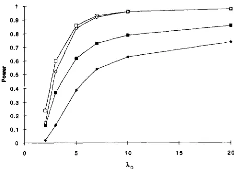
FIGURE 1.-Comparison of the power as a function of X. of simultaneous search to detect linkage to both loci ( 0 ) with the power of single locus search to detect linkage to at least one locus ( O ) , to a particular locus ( W ) , and to both loci ( ) for 200 sib pairs.

case of half siblings. For siblings the formula (23) holds with

EL

= ( N / 2 ) l / p a t .

The power of this test to detect linkage to chromosomes kl and

112

is

~{2"/'[rnax

z(kl,

s)

+

max

Z(b,

t ) ] 2 6)

,

1

= P(2"/2[Z(k1, 7 1 )

+

Z(b, ~ p ) ] 2 6)

+ P{2"/"Z(kl,

7 1 )

+

Z ( k 7 , 7 2 )

I

<

6,

Z"/'[max Z ( k l , s)

+

max Z ( b , t ) ] 2 b } . (24)

The major part of this probability is the first term after the equality, which is easily evaluated approximately by (23) and the central limit theorem. An approximation to (24) is given in APPENDIX

c.

Using this approximation, we compare the power of simultaneous search and single locus search in Figure

1. We assume there are N = 200 sibling pairs and a heterogeneous trait to which two unlinked loci make equal contributions. By (13) a = ( X o - 1 ) /2Xo. As a function of X(,, Figure 1 compares the power of simultaneous search to detect linkage to both loci with the power of single locus search to detect linkage to at least one locus, to a particular locus, and to both loci. Roughly speaking, the power of simultaneous search to detect linkage to both loci is slightly smaller b u t comparable with the power of single locus search to detect linkage to at least one locus, substantially larger than its power to detect linkage to a particular locus and larger still than its power to detect linkage to both loci.

Additional calculations not shown here indicate that although the specific numbers change, comparable results hold for other relative pairs, for the more general model ( 1 )

,

for traits involving three loci, and for cases where the various loci make unequal contributions to trait susceptibility (cf. DUPUIS 1994). It seems fair to conclude that if our goal is to establish the genetic char-

(8)

acter of a trait by demonstrating linkage of some sort, then simultaneous search does not have clear advantages nor disadvantages compared with single locus search.

The situation becomes more complicated if our goal is to detect all major loci, perhaps also to determine the number of major loci, to estimate the relative mag- nitude of their contributions, the mode of their interaction if any, etc. We continue to consider the simple case that there are (exactly) two loci making equal contributions to the trait. Although Figure 1 suggests that simultaneous search is much better than single locus search in detecting linkage to both major loci, a closer examination shows that this apparent virtue is confounded by the risk of also detecting spurious unlinked loci. To see this, consider the event that

max[max Z ( k l , s ) , max

Z(h,

t ) ]

5 t

+

max max Z ( j , t ) 2 2l"b,

j f k l , k z t

min [ max Z ( k,, s ) , max Z (

b,

t ) ]

S 1

<

max max Z( j , t ) . (25)

j * k l , k z t

This event describes the possibility that the apparently more important of the two linked chromosomes in conjunction with at least one of the unlinked chromosomes exceeds the threshold for detection, whereas the apparently less important of the two linked chromosomes gives less evidence for linkage than at least one of the unlinked chromosomes. If this occurs we will at best recognize that we cannot tell which is the second linked chromosome, and if we make the "obvious" choice we will choose incorrectly. The event (25) in effect identifies a different false-positive error from the one we have already discussed and controlled by the choice of the threshold b . If the probability of ( 25) were small, it would not concern us, but unfortunately it can be large enough to be worrisome.

From ( 13) and Figure 1 we can infer that a range of particular interesting values of =

E2

is from -3.3 to 5.0, where we can reasonably expect to detect at least one locus and are not certain to detect both. Based on an approximation in Appendix C, we find that over this range the probability of ( 25) varies between -0.25 and 0.05. [This probability could be much larger if [I f [2, although for a given average value

(5,

+

Se)

/ 2 it does not change substantially if the difference

15,

- 5 2 1 is

less than about one standard deviation.]

By similar reasoning, if we permit ourselves to detect

only two loci in a simultaneous search, the probability to detect the two trait loci is in reality less than (24) by virtue of the possibility that the maximum of the search statistic over some unlinked chromosome can exceed the lesser of the two maxima over linked chromosomes. This stricter definition would reduce the power in (24) by roughly the same amount that the false-positive error rate is increased. For a numerical example, suppose that we have

N = 200 sib pairs and X. = 5, so by ( 1 3 )

<,

=

t2

= 4.0. Then the false-positive error defined in ( 25) has about a

0.20 chance to occur, and although the probability of (24) is -0.83, the probability of correctly detecting the

two linked chromosomes and ranking them ahead of all unlinked chromosomes is only -0.68.

To carry this reasoning to a ridiculous extreme, if we were certain there are exactly two major loci, we might consider a single locus search where if at least one locus is detected we automatically declare that the chromosome giving the second highest maximum also contains a linked locus. We can define a false-positive error rate for this procedure similar to (25) and at the same time consider the probability of correctly detecting the two linked loci. The properties of this procedure would be essentially in- distinguishable from those of the simultaneous search discussed above. We have omitted the calculations.

One can imagine other situations where simultaneous search leads to ambiguous results. It seems fair to conclude that while simultaneous search holds out interesting possibilities, as implemented in (21 )

,

it is an inadequate solution to the complex problem of detecting all major loci (and only those loci).

Rmzark 2: It is natural to ask whether the problems identified here for simultaneous search also afflict the simultaneous search of LANDER and BOTSTEIN ( 1986), which was LOD score based. Although the differences in detail of the two methods make it problematic to speculate in the absence of detailed analysis, it does seem reasonable to note that the problems we have identified are based on questions that LANDER and

BOTSTEIN did not ask. For example, when they conclude that simultaneous search is substantially more powerful than single locus for detecting linkage, their comparison is with the power of single locus search to detect linkage to a particular locus. If we had limited ourselves to that comparison, we would have reached a similar conclusion. (We are assuming that the LOD score single locus search includes a heterogeneity parameter; otherwise it can lead to the well-known embarrassment of a negative LOD score while testing a marker at a trait locus.) Also, LANDER and BOTSTEIN did not consider the

problem of overdetection, ie., of detecting spurious unlinked loci in addition to the trait loci.

Remark 3: The simultaneous search statistic discussed above has the virtue that it is the score statistic

(Cox

and HINKLEY 1973, chap. 9 ) for both the additive and multiplicative models and seems reasonable for the much larger class of models given by ( 1 )

.

An

alternative is the likelihood ratio statistic, which is, however, model dependent. For the additive model, for half sibling pairs the likelihood ratio statistic is essentially based on (XI,

(9)

Linkage Analysis of Complex Traits 851

more powerful. For example, for X. = 10 and sibling pairs a crude analysis suggests that the likelihood ratio statistic would achieve the same power as the score statistic to detect at least one locus with -90% of the sample size. This increased efficiency would be greater for larger Xo, but smaller if more than two loci are involved. It appears that to realize the full strength of simultaneous search, one must use a model-dependent strategy and be favored by special circumstances.

Conditional search: If linkage to at least one chromosome has already been detected but the detected loci do not seem to account for the total incidence of the trait, it is possible to try to remove the effect of the loci already detected and search again to detect linkage to at least one more locus. There are at least three different contexts in which this problem might arise: ( 1 ) an earlier study has detected linkage to one or more major

loci, and we now want to analyze data from a different study; (

2 )

we have collected data sequentially and have already detected linkage to some loci in an earlier phase of the study; and ( 3 ) we have performed a preliminary analysis, for example, a single locus search, and have detected linkage to some loci and would like to continue analysis of the same data to find evidence for linkage to other loci. The second and third cases are complicated by problems involving reuse of the same data. We begin by discussing the first case.

Suppose that there are two trait loci, one at locus

T~ on chromosome k1 and the other at locus T~ on chromosome

122

f k l . Suppose also that linkage has already been established for chromosome k l , and the trait locus is thought to be at a point t, , not necessarily equal to T ] . For a grandparent-grandchild or half sibling pair, we find from ( 8 ) and Remark 1 that

P(X(122,

4 )

= 1

I

X(k1, t , ) = 11

= (1

+

[ a z ( 4 )

+

~ ( 4 ,

4)1/

[1

+ & 1 ( 4 ) 1 1 / 2 ( 2 6 )

and

PIX(122,

4 )

= 11 X ( k 1 , t l ) = 01

= (1

+

-

Y ( ~ I ,

4)1/

[1 -

a 1 ( 4 ) 1 1 / 2 , ( 2 7 )

where d, =

1

t, - T~

I

is the genetic distance between

the marker and trait locus. This means that in a sample of size N , if we consider only the subset of size

X

( kl ,

t l ) of pairs that are identical by descent at t l , then for this subset the identity by descent process on the remaining chromosomes behaves exactly like the original process, except that its sample size is now X ( kl

,

tl ) ,

and the parameter az has been replaced by [ az ( 0 )

+

y ( 4 , 0 ) 1 / [ 1 +al(dl)].Thesituationisthesameif

we consider the N - X ( kl

,

tl ) pairs not identical by descent at tl , except that now a2 is replaced by [ a2 ( 0 )

-

~ ( 4 , 0 ) ] / [ 1

-

a 1 ( 4 ) ] . It is easy to see that in

some cases, for example, in the additive case, so y =

0, when we condition on those pairs that are not identical by descent at t l , the new effective value of a z can be considerably larger than the original value, although the effective sample size may be considerably smaller. In addition, we have the presumably larger subgroup of pairs that are identical by descent at tl but whose effective value of a p has been reduced by conditioning. For a multiplicative model, the conditional probabilities in

( 2 6 )

and

( 2 7 )

are exactly the same as the unconditional. This means there is absolutely nothing to be gained by conditioning in the case of a gene interaction following a multiplicative model and presumably little to be gained in the case of a multiplicative model with phenocopies, unless the phenocopy rate is relatively large so that y is substantially larger than aIa2. For simplicity we assume in what follows that y = 0. It is perhaps also worth noting that a similar strategy to one we develop below has obvious appeal and has been discussed by a number of authors ( e.g., JANSEN 1993)

for linkage of quantitative trait loci in backcrosses and intercrosses of inbred strains. In that situation, however, in the absence of epistasis regression estimates associated with loci on different chromosomes are approximately independent and hence essentially uninflu- enced by conditioning, but one nevertheless obtains via conditional search a gain in efficiency by virtue of a reduction in the variability of those estimates.

Very similar results are easily obtained from ( 12) for the case of siblings. An important difference, however, is that for an additive (within loci) model, for those pairs having identity by descent on exactly one chrome some at tl

,

the conditional probabilities at

4

are exactly the same as the unconditional probabilities. This means that for a subset of the sample of sib pairs, constituting about 50% of the entire sample, there is nothing to be gained by conditioning. Consequently, the overall value turns out to be slightly less than for other relative pairs, as we see below.

To combine the data from each of these subsets, we consider the score statistic for testing the hypothesis that a z = 0 with a 1 considered to be an unknown nui- sance parameter. We fix tl and t on chromosomes kl

and k , and we assume these are the true trait loci. We obtain the score statistic for testing a2 = 0 against the alternative az

> 0

and then search over the possible values of t on all chromosomes k f kl while holding tl fixed. Initially, we also assume that a1 is known. For grandparent-grandchild or half sibling pairs the log likelihood function is given by (14) (with y = 0 ) . The score statistic is the derivative with respect to az evaluated at a2 = 0 and standardized to have unit variance

when az = 0. The result is

( 1 - a : )

(2x11

-

XI.)

(10)

the hypothesis that

as

= 0. Under this hypothesis the maximum likelihood estimator of ( 1

+

a l )

/ 2

is the proportion of pairs identical by descent at t l , namely

N-’

X,.

.

The statistic to be used in searching for a second linkage is

A number of fundamental insights into the behavior of ( 29) follow directly from ( 28)

.

First, ( 28) shows that (29) is intuitively quite reasonable because it combines the two comparisons suggested in (26) and

( 2 7 ) ,

namely those pairs identical by descent at the second locus among those identical by descent at the first and those pairs identical by descent at the second locus among those not identical by descent at the first. More- over, it gives greater weight to the second comparison, which was shown above to be the more informative. On unlinked chromosomes (28) is a weighted average of

two statistics that conditionally given X,. are essentially the same as the score statistic ( 18) and are independent. Hence, the same threshold b can be used to control the false-positive error rate. On linked chromosomes the expected value of

(28)

is N”*a2/ (1 - a ; ) ’ ’ 2 , and for small

a p

the variance is about equal to one. Because this mean value always exceeds N’/*a2, which is the expected value of the single locus statistic ( 18) at the second trait locus, conditional search leads to a gain in efficiency compared with single locus search. The ratio of these

two expectations is 1

/

( 1 - a : ) ‘ I 2 . Because the power of (29) and of single locus search to detect linkage to the second trait locus depends primarily on these expected values and because the expected values are proportional to

N’/‘,

use of conditional search has roughly the same effect as increasing the sample size by the factor 1

/

(1

- a : ) , which can represent a substantial increase in efficiency when a , is large. For a simple numerical example, suppose X. = 10, N = 144, a1 = 0.55, and az =

0.27 [ cf. ( l o ) ] . The more important locus, which is essentially certain to be detected by a single locus search with b = 4.08, contributes twice as much “signal” as the secondary locus. The power of the single locus search to detect the second locus is only -0.34. The approximation (28) indicates that the power of a conditional search based on (29) is -0.57. An -40% larger sample size would be required to achieve this power with single locus search.

One can easily obtain similar results for other pedigrees. For sibling pairs the score statistics analogous to (28) and (29) are easily computed and indicate an efficiency gain for conditional search of 1/2

+

’/*

( 1

-

a : )

-’.

For those pairs that are identical by descent on exactly one chromosome at the first trait locus, which is roughly one half the total number of pairs, there is no gain in efficiency, whereas the gain among that half of the sample having identity by descent on either none or both chromosomes is exactly

as in the case of half sibling pairs. Thus the overall gain in efficiency is less than for half sibling pairs. By ( 13)

the values of 0.6 and 0.3 for al and a2 correspond to the value X 0 = 10 and the same two to one relative importance as above. A sample size of

N

= 234 siblings leads to the same power as above, 0.34, for single locus search to detect the second trait locus. The approximation corresponding to (28) indicates that the power of conditional search is -0.49. About a 30% larger sample size would be required to obtain this power with single locus search.

The cases of more distant relatives and pedigrees containing more than two affecteds are particularly interesting. The primary source of the effectiveness of conditional search is the part of the total sample that are not identical by descent at the first locus. For second-degree relatives this is typically a small fraction of the total. For more distant relatives, for example, first cousins, where the probability of identity by descent at unlinked loci is only 1/4, even with a considerable enrichment for identity by descent at the first locus, there can remain a substantial fraction of the total sample who are not identical by descent there. In the case of larger pedigrees, it is likely that all affecteds within a pedigree have their trait by virtue of a common allele at one of the trait loci. This makes the stratification into subgroups of conditional search particularly effective.

For an example we consider first cousins and triples of half siblings, which have exactly the same statistical structure. For first cousins the log likelihood function is given by

x11log( 1

+

3al

+

x10 log( 1

+

3cY1

-

c Y 2 )

+

x 3 1 log (1 - a1

+

3a2)

+

X&

log( 1 - - ( ~ 2 ) . ( 3 0 ) For trios of half siblings one can incorporate the calculations of APPENDIX B of FEINCOLD et al. ( 1993) into our earlier analysis to obtain a log likelihood function of this same form, where now X,, is the number of trios for which all of the three possible painvise comparisons exhibit identity by descent at both loci, Xlo is the number for which all of the painvise comparisons show identity by descent at the first locus, but only one shows identity by descent at the second, etc. For first cousins the equation corresponding to ( 10) and ( 13 ) is

( ~ 1

+

= ( X 0

+

l ) / ( A o

+

3 ) ;

for trios a more complicated expression involving the first three moments of the penetrances is involved. An

analysis along the lines described above indicates an efficiency gain of

’/*

( 1

+

3a1)

-’

+

3/4( 1 - a , ) - ’ . In the case of first cousins the values of a , and ap corresponding to the previous examples ( i e . , 10 = 10) are 0.46 and 0.23, respectively, and the increase in efficiency of conditional search is -50%.

(11)

Linkage Analysis of Complex Traits 853

eter X. does not have a simple relation to the a's along the lines of ( 10) and ( 1 3 ) . For an example, expressed directly in terms of allele frequencies and penetrances we take two alleles at each locus. The frequencies of the disease susceptibility alleles are = 0.018 at the first locus and = 0.009 at the second; the penetrance of these alleles is f (at both loci), and there are no phenocopies, so the penetrance for the other alleles is zero. By extending the analysis of APPENDIX B of FEIN-

GOLD et al. ( 1993)

,

one calculates that X 0 = 10, a 1 =

0.55, and az = 0.28, and hence a gain in efficiency of -75%. The corresponding analysis for sibling trios indicates an efficiency gain of '/I,( 1

+

3al)

-'

+

3/8( 1

+

cy1 )

+

1 -

al

) - I . The same allele frequencies and penetrances yield the same a ' s in this case and hence a gain in efficiency of -50%. In both cases the gain in efficiency for trios is greater than for pairs,

as expected. For a slightly different example, let

pl

=

0.01,

p,

= 0.005, f = 0.5, and assume that phenocopies occur with probabilityfo = 0.005. Thus the incidence of phenocopies is the same as the incidence of cases due to the second locus. Again ho = 10. The a ' s are slightly larger than in the preceding example, so the gain in efficiency is also slightly larger.

This analysis is easily extended to heterogeneous traits involving three loci. For example, for half siblings, ifwe have detected and condition on two loci character- ized by the parameters a 1 and a2, the gain in efficiency of conditional search in searching for linkage to a third locusis'/2{[1 - ( a l + a 2 ) * ] - I + [I - ( a , -a2)*]-l).

We have assumed in the preceding calculations that the first trait locus is known exactly. If our estimate of its location is incorrect by d cM, as we see from (26) and (27) the value of a 1 in our efficiency calculations must be replaced by al exp ( - p d )

,

which will result in some loss of efficiency.

The situation is much more complicated in the case that we propose to use conditional search as a second phase in an analysis where a first phase consisting of single locus search has detected linkage to at least one chromosome. In addition to the problem mentioned above, that the original single locus search will not have identified the first trait locus exactly, because of the search procedure the proportion of pairs identical by descent at the detected locus will be a biased estimator of the probability of identity by descent at that locus. The effect of this bias might possibly degrade the efficiency gain suggested by the preceding calculation.

Also, the conditional phase of the search introduces new opportunities to make false-positive errors, so if one wants to control the overall false-positive rate for both phases to a prescribed level, say 0.05, it would be necessary to set the threshold b higher than for a single locus search that is not followed by a conditional search. This problem might become particularly acute if we were to implement a sequence of conditional phases.

It is not clear, however, how serious the effect on the false-positive error rate is. If we assume that we have an

O'*

I

0.7

o.2

0.1

Y

0 , I I

0.3 0.4 0.5 0.8 0.7

a1

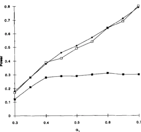
FIGURE 2.-Comparison of the power as a function of a 1

of single locus search

(m)

with conditional search (theoretical

+,

simulated 0) for 144 half-sib pairs.

idea of the value of ho from previous family studies, we presumably would only apply conditional search in those cases where the loci already detected are insuffi- cient to explain the value of

Xo.

Because a previous single locus search will already have failed to detect the remaining linked loci and because

(as

is easily shown) the conditional search statistic (28) is positively corre- lated with the single locus search statistic on unlinked chromosomes, it is plausible to think that the increase in the false-positive rate might be relatively small.

To investigate this situation, we conducted a simulation experiment for N = 144 half sibling pairs. We used the same threshold, b = 4.08, that we have used for

earlier theoretical calculations. Because this threshold is based on a normal approximation and because the data are actually discrete, for the single locus search, the nom- inal threshold b = 4.08 translates to a declaration of linkage when at least 97 of the 144 pairs are found to be identical by descent at some locus, and this converts back to a true threshold of 4.17 in the scale of the score statistic Z ( i, t ) in ( 18). The Gaussian approximation of Appendix A with b = 4.17 gives a false-positive error rate of 0.036, whereas the presumably more accurate Markov chain approximation of FEINGOLD ( 1993) with a threshold of 97 indicates that the true false-positive rate of the single locus search is -0.032. This latter value was

confirmed by our simulations, which also showed the conditional phase adding roughly an additional 0.01, so the overall false-positive rate is -0.04. It seems fair to conclude that the increase in the false-positive error rate

as a result of the conditional search is not a serious problem and probably can be ignored, unless one plans to iterate the conditional phase; and then caution suggests that the problem be studied more carefully.