ABSTRACT
BACHMEYER, PAUL. Simulation-Based Design Strategies for Component Optimization in Steer-by-Wire Applications. (Under the direction of Dr. Gregory D. Buckner.)
The objective of this thesis is to develop simulation-based design strategies for optimizing the selection of active,
semi-active, and passive components for industrial steer-by-wire (SBW) applications. Experimental steering data is
collected from an instrumented Honda Accord (1987 model) and used to validate a lateral vehicle model. This
model is used to investigate the tactile feedback performance of various SBW configurations at specific driving
conditions. Although peak performance is obtained with fully active components (direct-drive electric motors),
comparable performance can be obtained using a combination of passive springs, semi-active dampers, and active
Simulation-Based Design Strategies for Component Optimization in
Steer-by-Wire Applications
by
Paul Joseph Bachmeyer
A thesis submitted to the Graduate Faculty of North Carolina State University
in partial fulfillment of the requirements for the Degree of
Master of Science
Mechanical Engineering
Raleigh, North Carolina
2008
APPROVED BY:
Paul I. Ro Larry M. Silverberg
Gregory D. Buckner Chair of Advisory Committee
DEDICATION
This thesis would not have reached completion without the constant support and encouragement from my
girlfriend, Iris, my family, and my friends. Sacrifices beyond that which should be asked of loved ones were made
BIOGRAPHY
Paul Bachmeyer was born in Charlotte, NC in 1975. The love of his early life, his Lego’s, helped to develop a found
appreciation for creating that which was not. He awoke from his adolescence and found himself with a B.S.M.E.
His efforts to determine if there truly was anything that doughnuts could not do were fruitless; therefore, he
ACKNOWLEDGMENTS
This work was supported by LORD Corporation. I would like to thank all of those (too numerous to list here) that
provided assistance to my research. I would like to thank my advisor, Dr. Gregory Buckner, for his patience and
willingness to help complete this work in such a timely manner. His guidance and assistance along the way was
beyond the call of duty. I want to thank Dr. Donald Margolis for his constant support with bond graph modeling
and the research feedback related to vehicle dynamics. Finally I want to thank all of my committee members for
TABLE OF CONTENTS
LIST OF TABLES ...vi
LIST OF FIGURES ...vii
1 Introduction ... 1
1.1 Aims of this Study ...7
2 Methods and Materials...9
2.1 Vehicle Dynamic Modeling...9
2.2 Overview of Bond Graph Modeling ...11
2.3 “Bicycle Model” ...12
2.4 SBW Active and Semi-Active Components...17
2.4.1 Active : Electric Motor ...17
2.4.2 Semi-Active: Magnetorheological Tactile Feedback Devices (MR Brakes) ...17
2.5 Experimental Test Set-up...20
2.5.1 Model Parameter Acquisition...23
2.5.2 Model Parameter Calculation ...23
2.6 Experimental Test Conditions ...25
3 Results... 27
3.1 Vehicle Test Results ...27
3.1.1 ISO 3888-1 Test Track ...27
3.1.2 Normal City Driving ...31
3.1.3 Comparison of Experimental and Simulation Results...33
3.2 Basic Design Strategy for SBW Component Selection ...37
3.2.1 Passive Component Selection Strategy ...37
3.2.2 Active and Semi-Active Component Selection Strategy...39
3.2.3 Active Component Selection...42
3.3 Comparison of Selected Steer-By-Wire Component Combinations...43
3.3.1 Fully Passive ...45
3.3.2 Fully Active...50
3.3.3 Fully Semi-Active...51
3.3.4 Passive/Semi-Active ...53
3.3.5 Passive/Active...54
3.3.6 Semi-Active/Active...56
3.3.7 Passive/Semi-Active/Active...57
4 Discussion ... 59
5 Conclusions ... 62
6 References ... 64
7 Appendices ... 66
7.1 Road Testing Locations...67
LIST OF TABLES
Table 1: Bond graph effort and flow quantities...12
Table 2: Vehicle parameters for model analysis...24
Table 3: ISO 3888-1 road course dimensions for double lane change ...26
Table 4: Spring stiffness for a passive component for SBW...38
Table 5: Spring design information for passive component of SBW ...39
Table 6: LORD 5 Nm TFD™ component information [9, 27]...42
Table 7: Moog BN-34 series BLDC component information [30] ...43
Table 8: Comparison of SBW design options and system performance at 48 kph...47
Table 9: Comparison of SBW design options and system performance at 64 kph...48
LIST OF FIGURES
Figure 1: (a) Hydraulic power system (components 1-4, 7-8 parts of the hydraulic/cooling circuit), (b)
Electro-hydraulic power steering system [1] ...2
Figure 2: Electric power steering system (a) steering column assembly, (b) vehicle installation [1]...2
Figure 3: Fly-by-wire applications to commercial aircraft: (a) A320, (b) FBW cockpit, (c) Falcon 7X [3] ...3
Figure 4: Application of GPS and controlled steering to agriculture equipment [6]...4
Figure 5: OEM equipment with SBW technology (a) Lansing Linde lift truck, (b) Volvo Penta [10, 11] ...5
Figure 6: Application of SBW to GM Sequel concept car (a) system configuration, (b) Driver Interface System (DIS) [4]...6
Figure 7: GM Sequel end stop control [4] ...6
Figure 8: Diagram of tire slip angle...10
Figure 9: General lateral tire force versus slip angle [19] ...11
Figure 10: Bicycle model with steering input for model simulation...13
Figure 11: Completed bond graph of a "bicycle" model vehicle with conventional steering...15
Figure 12: TFD™ component schematic (a) embodiment of assembly [26], (b) working cross-section ...18
Figure 13: LORD Corporation 5 Nm TFD™ component (a) device [9], (b) torque versus current [27] ...19
Figure 14: LORD Corporation 12 Nm TFD™ component (a) device [9], (b) torque versus current [27] ...19
Figure 15: LORD Corporation 12 Nm TFD™ component as function of input velocity and current ...20
Figure 16: Steering cradle, torque cell, string pot, and cradle installation ...21
Figure 17: Accelerometer vehicle installation...22
Figure 18: Data acquisition and power supplies ...22
Figure 19: Vehicle weight determination for CG location...23
Figure 20: Double lane-change road course and section designations ...25
Figure 21: Overlay of acquired vehicle data, 48 kph...28
Figure 22: Overlay of acquired vehicle data, 64 kph...29
Figure 23: Overlay of acquired vehicle data, 97 kph...30
Figure 24: Overlay of acquired vehicle data, normal city driving ...32
Figure 25: Lateral acceleration versus time, 48 kph ...34
Figure 26: Steering torque versus time, 48 kph...34
Figure 27: Steering torque versus steering wheel angle, 48 kph...35
Figure 28: Steering wheel torque versus steering wheel angular velocity, 48 kph. ...35
Figure 29: Mechanical steering power versus time, 48 kph. ...36
Figure 30: Power versus steering wheel angle, 48 kph...36
Figure 31: Passive element determination...38
Figure 32: Required steering torque (total measured and spring-augmented) vs. steering wheel angular velocity: 48 kph ...41
Figure 33: Sorting algorithm for generating SBW tactile feedback torque from vehicle torque...44
Figure 34: Fully passive SBW feedback torque vs. measured steering torque: 48kph, Run 2 ...46
Figure 35: Fully active SBW feedback torque vs. measured steering torque: 48kph, Run 2...50
Figure 36: Fully active SBW current: 48kph, Run 2 ...51
Figure 37: Generated SBW feedback torque with damper element only: 48kph, Run 2...52
Figure 38: Current for SBW feedback torque with damper element only: 48kph, Run 2 ...52
Figure 39: Generated SBW feedback torque with spring and damper elements: 48kph, Run 2...53
Figure 40: Current for SBW feedback torque with spring and damper elements: 48kph, Run 2 ...54
Figure 41: Generated SBW feedback torque with spring and motor elements: 48kph, Run 2 ...55
Figure 42: Current for SBW feedback torque with spring and motor elements: 48kph, Run 2...55
Figure 43: Generated SBW feedback torque with motor and brake elements: 48kph, Run 2 ...56
Figure 44: Current for SBW feedback torque with motor and brake elements: 48kph, Run 2...57
Figure 45: Generated SBW feedback torque with spring, motor and brake elements: 48kph, Run 2 ...58
Figure 47: Average required SBW electrical energy: 48kph ...60
Figure 48: Average required SBW electrical energy: 64kph ...61
Figure 49: Average required SBW electrical energy: 97kph ...61
Figure 50: Driving location for ISO3888-1, 48 and 64 kph...67
Figure 51: Driving location for ISO3888-1, 97 kph...67
1 Introduction
Although the operation of an automobile is a familiar experience to most adults, its complexities are seldom
contemplated. Lateral control of an automobile requires simultaneous processing of visual, audible, and tactile
feedback signals. The steering wheel serves as the sole input device for lateral control, and tactile feedback is
provided through direct mechanical connections to the vehicle’s front wheels. While totally electronic controls have
been adopted in aerospace markets, the benefits of steer-by-wire technologies have yet to be realized in the
automotive realm.
Early automobiles provided no mechanical assistance for steering, which made turning at low vehicle speeds
difficult. Developed in the mid 20th century, power steering systems coupled hydraulic actuators with the manual
direct drive steering components to provide steering assistance. Hydraulic power steering became commercially
available in 1951, and became a standard feature of automobiles in the 1980s [1]. Power for the hydraulic pump is
provided directly from the engine using a belt and pulleys. Figure 1a illustrates the components of a typical hydraulic
system. The electro-hydraulic power steering system (Figure 1b) uses an electric motor, (Component 1) rather than
the engine, to drive the hydraulic pump. This system has several advantages over previous designs in that it allows
for more flexibility in its location, requires no cooling circuit, provides steering boost even when the engine is not
(a) (b)
Figure 1: (a) Hydraulic power system (components 1-4, 7-8 parts of the hydraulic/cooling circuit), (b) Electro-hydraulic power steering system [1]
Like electro-hydraulic systems, electrical power steering (EPS) systems employ electric motors to provide assisted
steering, but completely eliminate the use of hydraulics. Benefits of EPS include: increased performance, reduced
environmental concerns associated with fluid leakage, decreased power consumption, and enhanced tuning for
desired performance. Other benefits include greater flexibility in the placement of components (parts can be placed
oriented in a variety of directions) and the ability to provide steering assistance when the engine is powered off
[1, 2]. Figure 2 shows an EPS installed in an automobile [1].
(a) (b)
Similar and arguably greater advances in vehicle control have been made in the aerospace industry with the
development and extensive use of fly-by-wire (FBW) technology. FBW technology replaces traditional flight
controls (direct mechanical linkages such as wire rope and push rods) with actuators controlled electronically by the
pilot. In 1972, NASA introduced digital FBW control using an F-8C Crusader test bed. The application of FBW
technology to large commercial aircraft began in 1985 with the Airbus A320 and penetrated the business jet market
in 2005 with the Dassault Falcon 7X [3]. FBW systems are now commonly employed by all sectors of modern
aircraft.
(a) (b) (c)
Figure 3: Fly-by-wire applications to commercial aircraft: (a) A320, (b) FBW cockpit, (c) Falcon 7X [3]
Despite its widespread use in the aerospace industry, similar technologies have yet to be widely adopted by the
automotive industry. The automotive equivalent of FBW, steer-by-wire (SBW) technology, replaces mechanical
linkages of the steering system with electrical actuators, controllers and sensors [4]. SBW offers many advantages
not available with current automotive steering systems: assisted steering for parallel parking, collision avoidance,
lane tracking, increased stability control, and variable steer ratios [4]. By removing the traditional steering column
and linkages, additional space can be provided for other design features or for improved layout of the engine
compartment. Another advantage of SBW is decreased fuel consumption due to the elimination of continuously
driven loads typical of hydraulic steering systems, which can exceed the loads of air conditioning systems. The
SBW also offers potential advantages to agricultural industries. Research involving “intelligent SBW tractors”,
which combine electro-hydraulic steering components with GPS sensors and controllers, is enabling autonomous
steering while the “driver” monitors secondary tasks such as seed planting and crop harvesting (Figure 4). Such
systems would allow for increased fuel efficiency, multiple work functions in a single pass, and reduced overlap.
Figure 4 shows one embodiment (artist rendition) of the system [6].
Figure 4: Application of GPS and controlled steering to agriculture equipment [6]
One shortcoming of SBW systems is their inherent lack of haptic feedback to the driver. With conventional
steering systems, tactile feedback is mechanically transmitted through the tire’s interaction with the road surface,
through the steering linkages and steering wheel to the driver. Because they lack a direct mechanical connection
between the wheels and steering wheel, however, haptic feedback in SBW systems must be artificially generated.
This inherent lack of feedback presents obstacles to widespread commercial adoption of SBW, but it also offers
potential benefits: artificial haptic feedback can be “tuned” independently of tire selection, bushing stiffness, caster
distance, and camber angle, allowing for greater design flexibility [4].
The benefits of haptic feedback can be seen in technology under development by the manufacturers of reach and
lift trucks. One patented design employs both active and semi-active components coupled with position sensing
devices [7]. Another lift truck technology combines passive springs to generate restoring moments with a
magnetorheological (MR) device for resistive torque [8]. Such systems can be easily tuned to change parameters that
and at what rate it is applied and where it begins to be employed [8]. The haptic feedback can be tuned to achieve
any performance desired and one system with multiple tuning options controlled in software can be used across
various vehicle platforms [7]. Material handling equipment manufacturers such as Fenwick, John Deere, and
Lansing-Linde use MR brakes to provide tactile feedback to the operators of forklifts. TFD™ components are used
in safety-critical marine-propulsion applications such as the Volvo Penta IPS steering system [9]. Figure 5 shows
various applications of these technologies.
(a) (b)
Figure 5: OEM equipment with SBW technology (a) Lansing Linde lift truck, (b) Volvo Penta [10, 11]
In the automotive industry, haptic feedback devices are already used for secondary interface controls for audio,
climate, navigation, and telecommunications systems. Such interfaces typically use an electrostatically responsive
fluid (ERF) that changes its viscosity in response to electrical stimulation. ERF allows control of multiple functions
with a single mechanical interface, since feedback can be made to emulate any desired feedback. ERF devices allow
for smaller size and sufficient torque compared to an electric motor or MR device combination [12].
The adoption of SBW in the automotive industry is also hindered by safety, security, and cost issues. Electronic
components of SBW systems frequently lack the reliability of mechanical components of traditional steering
Steering control unit using SBW
mechanisms. Therefore, redundancy or other measures must be provided to prevent catastrophic failure of SBW
systems, possibly raising costs and reducing reliability [4].
Because of these technical challenges, the introduction of SBW technology into the automotive industry is limited
to concept cars such as the GM Sequel [4]. The Sequel test bed uses a standard steering wheel interface (joystick
controls are other design options), a brushless DC motor with 4:1 ratio belt drive, and an MR brake for end stop
and passive steering resistance (Figure 6). Research and development efforts focused on security and fault tolerance
objectives through the use of three absolute position sensors and a mechanical steering backup system. The system
shows that the torque of the steering wheel can be generated by the motor and the MR brake in unison for such
design functions as end stop control (Figure 7).
(a) (b)
Figure 6: Application of SBW to GM Sequel concept car (a) system configuration, (b) Driver Interface System (DIS) [4]
Effective SBW technology requires not only appropriate hardware but also adequate control algorithms.
Researchers have developed control algorithms considering both the steering angle and the steering torque [13]. In
a study by Kleine et al., control evaluations were conducted using computer simulations; the study included no
experimental data from actual vehicles and no comparison of steering torque between the real and modeled
vehicles. Yuhara, et al. analyzed the tradeoffs of a SBW steering system controller with respect to tracking
performance, disturbance rejection and insensitivity to measurement noise. Simulator tests were used to validate the
models. The use of artificial steering torque to improve vehicle handling using information from lateral position
error was discussed and showed that artificial steering torque feedback has some effect as a reduction of driver’s
measurement noise [15].
1.1 Aims of this Study
SBW technology has a broad range of applications in existing devices and the ability to enable new devices. In the
short term, penetration into the automobile market is desirable, but issues of safety and cost have thwarted the use
of this technology. Several key issues must be addressed before SBW is widely accepted by the automotive industry:
1) How much feedback torque should be applied by the SBW system?
2) What components should be used to replicate this feedback torque? Options include electric motors,
MR brakes, and mechanical springs.
3) If several components are combined, how is the feedback torque generation to be shared such that an
optimal feedback torque is generated with minimal power consumption and realistic tactile feedback?
The focus of this research is to determine optimal combinations of active, semi-active, and passive components to
components (rotary and linear motors) can be expensive, heavy, and require sophisticated control hardware, the
SBW system will be optimized for reduced cost, weight, and complexity. A dynamic vehicle model will be created to
predict the required feedback torque based on operating conditions and input parameters. A generalized SBW
2 Methods and Materials
2.1 Vehicle Dynamic Modeling
Simulation-based design and evaluation of SBW technology requires an accurate mathematical model of the vehicle
dynamics. Although automobiles exhibit coupled dynamic responses in six degrees of freedom (fore/aft, lateral,
vertical, roll, pitch, and yaw), this investigation will rely solely on the lateral and yaw motions for analysis and model
formation. Such models provide significant insight into the dynamics of automotive steering, and are well-studied
in the literature [16, 17, 18]. This model will be validated by acquiring experimental data (steering and forward speed
inputs, lateral acceleration outputs) from an actual vehicle and optimizing model parameters to maximize simulation
accuracy.
A ‘body-fixed’ coordinate frame is selected for model development. This coordinate frame is fixed to the vehicle’s
center of mass, aligned in principle directions, and moves with the vehicle. This model is often used with the
assumption of constant forward speed but this is not a requirement. State equations formulated for this system
provide velocity and acceleration of the vehicle, but not the vehicle position. Positional information can be readily
extracted by referring the body fixed outputs to an inertial frame. The modeling process is facilitated by assuming
that the lateral velocity is small compared to the forward velocity and that any velocity contribution from the yaw
rate is also small compared to the forward speed. These assumptions allow representation of a four-wheeled vehicle
using a two-wheel ‘bicycle model’: a single wheel at the front axle and a single wheel at the rear axle.
The interactions of pneumatic tires with the road surface are important to lateral vehicle dynamics, as steering
forces are created from the lateral reaction forces between the tire and road. If no lateral force is applied to the
front tire, then the vehicle will travel in a straight path. If a small lateral force is applied to the front tire, then some
lateral velocity will be imparted on the tire. The tire velocity vector will differ from the forward vehicle direction by
an angle known as the slip angle α (Figure 8), which rarely exceeds 10o for typical automobiles and driving
road surface, but rather that the contact patch (the area of interaction between the tire and road) moves with respect
to the road surface due to deformation of the tire. There can also be longitudinal slip due to braking and tire
traction, but these effects will not be considered in this investigation as the vehicle speed will be assumed to be
constant.
Figure 8: Diagram of tire slip angle
Because it is difficult to describe lateral tire/road interactions via first principles, most models are empirical fits to
experimental results (Figure 9). Lateral force and slip angle are linearly proportional over a limited range, assuming
the tire does not skid. The proportional constant for small slip angles (0-5o) is known as the cornering coefficient,
Cα. Other vehicle parameters like camber angle can affect lateral forces. However, because 1o of camber angle
generates much less force than 1o of slip angle, such dependences are ignored for this investigation [19].
α Original direction of travel
New direction of travel Top
View
Lateral force on vehicle α – slip angle
Contact patch Center of vertical
rotation (turn)
Figure 9: General lateral tire force versus slip angle [19]
The vehicle dynamics could be modeled using a number of techniques, including Newtonian mechanics or
energy-based models. Since SBW systems are inherently multi-domain, it is helpful to use tools specifically designed for
multi-domain systems, namely bond graphs. Principles of bond graph modeling are detailed in several textbooks
[16, 20, 21, 22, 23, 24]. Here, only a brief overview will be provided.
2.2 Overview of Bond Graph Modeling
Bond graphs are graphical descriptions of dynamic systems derived from conservation of energy principles. These
graphs consist of inductive, capacitive, and resistive elements from various energy domains interconnected by
power “bonds”, which establish the “effort” and “flow” variables of the system [24]. Power variables for a variety
of common energy domains are listed in Table 1. In all cases, it is obvious that instantaneous power is the product
of effort and flow:
f(t) e(t)
Table 1: Bond graph effort and flow quantities
Domain Effort, e(t) Flow, f(t)
Mechanical translation Force, F(t) Velocity, v(t)
Mechanical rotation Torque, τ(t) Angular velocity, ω(t)
Hydraulic Pressure, P(t) Volume flow rate, Q(t)
Electric Voltage, V(t) Current, i(t)
As with any system diagram, assumptions for positive and negative power directions must be clearly stated. This is
done in bond graphs by use of “half arrows”: a “half arrow” points in the direction of positive power flow, while a
“full arrow” indicates a signal flow of negligible power (a measurement). Bond graph convention requires that
effort variables reside above or to the left of power bonds while flow variables reside below or to the right of
bonds.
Power bonds interconnect the ports of various elements via “0” or “1” junctions, which designate constant effort
and constant flow, respectively. Because energy-storage elements (inductive and capacitive elements) cannot
simultaneously “cause” effort and flow, it is necessary to designate “causality” in interconnected elements and
junctions. Bond graphs use “causal strokes” (stroke perpendicular to one end of a power bond) to indicate
elements that define effort. Other bond graph elements, such as “flow sources”, “effort sources”, “transformers”
and “gyrators” can be included to model power sources and physical devices which alter the power variables. Once
a bond graph is properly constructed, it can be used to generate differential state equations for the system, given
constitutive relationships (linear or nonlinear) for each element.
2.3 “Bicycle Model”
A “bicycle model” of the lateral vehicle dynamics is presented in Figure 10. As mentioned previously, this model
model assumes a constant forward vehicle speed, and incorporates a conventional steering wheel to compute the
feedback torque.
Figure 10: Bicycle model with steering input for model simulation
A bond graph representation of this model is initiated by considering the energy-storage components, in this case
three mechanicalkinetic energy storage components: m (the vehicle mass), J (the vehicle mass moment of inertia), and
Jsw (the mass moment of the steering wheel assembly). Each of these components is associated with an ─I
(inductive) bond graph element and a 1-junction (constant flow), as shown in Figure 11. The remaining elements and
power bonds are added by considering the model kinematics. The driven wheel angular velocity, ωz, can be related
to the steering wheel angular velocity, ωsw, through the steering gain, gsw:
sw ω sw g z
ω = ⋅ (2)
The lateral velocities at the front and rear wheels can be determined by summing components of the vehicle
forward velocity, U, and lateral velocity, V:
δU z cω aω V f
v =− − + + (3)
bω V r
v =− + (4)
b a
V
U Fcr
Fcf
ω
m, J
ωz
c
Contact patch
δ Rear Tire
Front Tire CG
ωsw
Jsw
The cornering forces for the front and rear wheels are determined from the cornering coefficient and the slip angle:
U f C f v f C U
f v f C f cf
F =α ⋅ = ⋅ = ⋅ (5)
U r C r v r C U
r v r C r cr
F =α ⋅ = ⋅ = ⋅ (6)
When body-fixed coordinates are used, a modulated gyrator, ─MGY─, must be used. The modulated gyrator
accounts for the change in direction of velocity components referred to the body fixed coordinate frame. The
modulated gyrator modulus is, mω, as shown in Ref. [24]. Since the lateral dynamics are of interest in this paper,
only the summation of forces in the lateral direction is shown (7), but a similar result can be found for the forces in
forward direction. The modulated gyrator is used since the mω term is not constant.
∑Fy−mωU =mV& (7)
The feedback torque experienced by the driver is incorporated into the bond graph by recognizing that it is
generated at the tire/road interface and is transmitted through the kinematics of the steering system. This torque
can be added as a 0-junction at the location of the flow source, ωsw. It is also necessary to note that this feedback
torque requires zero power, i.e. it has no affect on the lateral dynamics.
At this point the bond graph is nearly complete, but in order to derive the state equations, causality must be
included. The assignment of causal strokes begins at source elements (Se, Sf) and propagates as far as possible using
constraint elements (0, 1, GY, TF) until all sources are assigned [22, 24]. Next, all energy storage elements
(─C’s and ─I’s) are assigned integral causality and carried through all constraint elements (0, 1, GY, TF). Applying
these basic rules of causal assignment and identifying the input and energy state variables yields the completed bond
Figure 11: Completed bond graph of a "bicycle" model vehicle with conventional steering
The bond graph of Figure 11 yields first-order, linear equations of motion in state space form:
Bu Ax
x& = + (8)
Du Cx
y = + (9)
+ + − − − − + − = sw ω δ sw cg U f C a f aC sw cg U f C f C J p V p JU ) r C 2 b f C 2 (a mU ) f aC r (bC J mU JU aCf) (bCr mU ) r C f (C J p V p & & (10) 0 1 TF1 Sf : ωsw
Jz : I
I : Jsw
τfb
TF: c
0
Cf/U : R
MTF: δ 1
Sf : U MGY 1
I : m
pv
1
I : J
pj
TF: b
0 R : Cr/U
TF : 1/a mω
ωz
gsw
V ω
. .
The feedback torque, τfb, is the torque that the driver of the vehicle senses on the steering wheel due to the
cornering forces imparted on the wheels coupled with the caster distance, c, and the steering gain of the steering
system, gsw.
) sw ω sw cg J J p a m V p (Uδ U f C ( sw cg sw ω 2 sw g τ b sw ω ) z J 2 sw g sw (J fb
τ = + & + + − − + (11)
An important parameter to be used in vehicle and model analysis is the lateral acceleration of the vehicle. An
expression for this can be derived from (7).
ω
U V lat
a = &+ (12)
The vehicle angular velocity and lateral velocity can be represented in terms of the state variables using the
definition for ─I elements:
J / p
ω= J , V = pV /m (13)
Substituting the relationships from (13), the expression for the lateral acceleration can be expressed in terms of the
momentum variables, the vehicle mass and inertia.
J p U m p lat
2.4 SBW Active and Semi-Active Components
2.4.1 Active : Electric Motor
The trend in the automotive industry is to replace mechanically actuated systems with electronic devices such as
motors [25]. Selection of the correct motor type and size is necessary for proper functionality of the system. DC
motors are common in these applications since their torque output is a linear function of the current applied.
Commutated DC motors are not ideal because of wear and arcing issues [2]. Brushless permanent magnet (BPM)
motors offer higher levels of efficiency and power density along with reduced torque ripple compared to other
motor options [2].
Because the electro-mechanical dynamics of brushless servo motors are several orders of magnitude faster than the
vehicle dynamics, for purposes of this study, it is acceptable to neglect the transient dynamics of the motor. As
such, a simple motor model is feasible whereby torque of the DC motor (τDC) is proportional to armature current
(ia) via a manufacturer-supplied motor constant, kτ:
τ = k × i
DC τ a (15)
And the electrical power
( )
Pe is determined via:a
2
P = i × Re
a (16)
Where Ra is the armature resistance.
2.4.2 Semi-Active: Magnetorheological Tactile Feedback Devices (MR Brakes)
Magnetorheological (MR) brakes are increasingly popular TFD™ components in steer-by-wire systems. These
continuously variable resistive torque that is a function of the applied current to the device. The response time of
these devices is on the order of milliseconds and provides a smooth and continuous feedback steering “feel” [26].
The MR TFD™ component also provides for a large operating and storage temperature range of -35oC to +70oC.
The MR TFD™ component is relatively compact and energy efficient allowing for a high torque density per unit
volume [27]. One OEM rejected the use of an electric motor for use as a feedback device because of the associated
cost, weight, size, and power consumption. An MR device was selected since it could provide the same torque in a
package 60% less than the electric motor [9]. Figure 12 shows how the typical components of a steering feedback
system are incorporated into a single TFD™ component.
(a) (b)
Figure 12: TFD™ component schematic (a) embodiment of assembly [26], (b) working cross-section
The MR TFD™ component also provides increased safety compared to electric motor feedback devices since the
MR TFD™ component does not provide any potentially dangerous high feedback torque to the operator. This can
also be a disadvantage if active torque feedback is required.
Housing
Bearing
Shaft
Rotor Stator
Coil
Figure 13 and Figure 14 show pictures as well as torque versus applied current curves for a 5 Nm and 12 Nm
TFD™ components, respectively, and features of size for reference [9, 27]. The torque-current curves show that
the devices are relatively linear over 67% of the stated current input range with saturation occurring at
approximately 1.5 Amps. The MR brakes also show little sensitivity to angular velocity (Figure 15) in terms of
torque output.
(a) (b)
Figure 13: LORD Corporation 5 Nm TFD™ component (a) device [9], (b) torque versus current [27]
(a) (b)
Figure 14: LORD Corporation 12 Nm TFD™ component (a) device [9], (b) torque versus current [27] 80mm
59mm
90mm
45mm
0.00 4.00 8.00 12.00 16.00 20.00
0 0.5 1 1.5
Current (Amp)
T
o
rq
u
e
(
N
m
)
30 RPM 60 RPM 90 RPM 120 RPM Poly Fit
Figure 15: LORD Corporation 12 Nm TFD™ component as function of input velocity and current
2.5 Experimental Test Set-up
To demonstrate the modeling and applicability of SBW, a 1987 Honda Accord DX was instrumented to acquire the
necessary parameters for comparison with the vehicle “bicycle” model. This particular vehicle was chosen for its
ease of modification and adaptation of test equipment and the lack of any electric power steering assist – only
hydraulic. The OEM steering wheel was modified to allow measurement of the driver’s input to alter the lateral
position of the vehicle. A steering cradle assembly consisting of a base, string pot pulley, reaction torque cell and
secondary steering wheel and adapter was attached to the OEM steering wheel as shown in Figure 16. Components
for the steering cradle were machined from aluminum and fastened together with standard hardware. The steering
cradle arms expand and contract in unison via a center disk and links. The arms are then clamped to the OEM
wheel with individual restraining tabs and bolts. The string pot pulley has a known radius of 48.96mm and was
used to convert the linear sting pot deflection to angular motion of the steering wheel. The torque cell
(S. Himmelstein & Co., Model 2137(2.2), 200lb-in) was rigidly attached between the string pot pulley and the
secondary steering wheel (McMaster Carr). The string pot (UniMeasure, LX-PA-40) was mounted to the front
Lateral acceleration of the vehicle was acquired from an accelerometer (Analog Devices, ADXL320EB, dual axis,
±5g) mounted on the car frame near the manual gear selector (Figure 17). The accelerometer selected was capable
of reading accelerations near 0g and at frequencies < 1 Hz. The accelerometer was attached to the vehicle as close
to the fore/aft location of the CG as possible. Since the model used to analyze the vehicle ignores the roll and
pitch effects of the vehicles dynamics, it was desired to place the accelerometer as close to the ground as possible to
minimize accelerations in those directions from affecting the desired lateral measurement.
Figure 16: Steering cradle, torque cell, string pot, and cradle installation Test input
steering wheel
OEM steering wheel
String pot Reaction
torque cell
String pot pulley
Figure 17: Accelerometer vehicle installation
The data was collected using an acquisition device (IOTech Wavebook 516, 8-channel, 16-bit) connected via parallel
port cable to a laptop computer (Dell Precision M60) with associated software. The torque cell signal was
conditioned with a differential amplifier/signal conditioner (Transducer Technologies, TMO-2) installed in the
passenger foot-well (Figure 18). Power for all electrical connections was supplied from a DC-AC inverter (Radio
Shack, 350W) connected to a power strip (Powerware, Net Surge Plus). Power (5V, DC) for the string pot and
accelerometer was provided with a DC power supply (BK Precision, model 1735A, 30V / 3A). The supply voltage,
accelerometer output at 0g, and the torque cell offset adjustment were verified with a digital multimeter (Fluke 87).
Figure 18 shows this equipment.
Figure 18: Data acquisition and power supplies IOTech
Wavebook
Laptop DC/AC Inverter DC Power Supply Power
Strip
2.5.1 Model Parameter Acquisition
The location of the fore/aft CG was determined from direct weight measurement of the vehicle. Both front wheels
were placed on individual scales (Intercomp, PT300, 5000kg) to determine the weight distribution on the left and
right front wheels (Figure 19) with the total front weight being the sum of the individual weights. The same
procedure was performed for the rear wheels. The wheelbase was measured using a standard tape measure
(Stanley, 10m).
Figure 19: Vehicle weight determination for CG location
2.5.2 Model Parameter Calculation
A few model parameters were calculated directly from measured vehicle data. The location of the vehicle CG from
the front and rear wheels was calculated as shown:
L W W
W a
r f
r
+
= L
W W
W b
r f
f
+
= (17)
Scale
Where, a is the distance from the front wheels to the CG, b is the distance from the rear wheels to the CG, L is the
wheelbase, Wf is the total vehicle weight on both front wheels, and Wr is the total vehicle weight on both rear
wheels.
The angular position of the steering wheel was calculated from the linear deflection of the string pot as shown:
1 1
− + − −
=
n sp
R n x n x
n θ
θ (18)
Where θn is the angular position of the wheel in radians and xn is the linear position of the string pot in millimeters
at time n, θn-1 is the angular position of the wheel in radians and xn-1 is the linear position of the string pot in
millimeters at time n-1 and Rsp is the radius of the string pot pulley in millimeters.
The parameters for the vehicle model (Equations 10 and 11) are shown in Table 2. These parameters were acquired
from published specifications [28], from measurements of the vehicle, and based on typical values and ranges for
difficult to measure parameters [16, 19].
Table 2: Vehicle parameters for model analysis
Parameter Symbol Value Units
Wheelbase L 2.60 m
Front wheel location from CG a 1.01 m
Rear wheel location from CG b 1.59 m
Vehicle mass m 1270 kg
Vehicle mass moment of
inertia J 673.6 kg-m2
Steering wheel mass moment
of inertia Jsw 0.088 kg-m2
Driven wheel mass moment
of inertia Jz 1.91 kg-m2
Caster distance c 0.047 m
Cornering coefficient, front Cf 50,863 N/rad
Cornering coefficient, rear Cr 38,906 N/rad
Understeer coefficient Ku 1.2 -
Steering damping bτ
375 (48, 64kph)
2.6 Experimental Test Conditions
The vehicle test input was based on the international standard ISO 3888-1 [29]. This standard describes a severe
double lane-change maneuver consisting of driving a vehicle from an initial lane into a parallel lane and then back to
the initial lane. Although the test is intended to analyze the lateral dynamics of the vehicle, there is inherent
variation in test results due to the operator as the path to follow and reaction times can vary from one operator to
the next. This standard was intended to provide a means by which data could be collected and repeated if
necessary.
Some modifications to the prescribed test course were implemented since the road course selected was an active
public roadway. Smaller cones than the ones specified were used to mark the beginning and ending positions of the
test segments along the curb of the road, but no cones were placed in the street. Chalk and the double yellow
center line were used to mark the test segments in these locations. The modified course (Figure 20) and its relevant
sections are defined in Table 3. The placement of the cones is indicated with green dots and the chalk marks are
indicated with orange dots.
Figure 20: Double lane-change road course and section designations
1 2 3 4 5 6
Lane
offset Width
Direction
Standard Center Lane Markers Imaginary Boundary of Road Course
Table 3: ISO 3888-1 road course dimensions for double lane change
Section Length (m)
Lane Offset (m)
Width (m)
1 15 - 2.11
2 30 - -
3 25 3.5 2.28
4 25 - -
5 15 - 2.45
3 Results
3.1 Vehicle Test Results
3.1.1 ISO 3888-1 Test Track
Measured data for the prescribed double lane change maneuver was acquired at three different forward vehicle
speeds: 48, 64 and 97 kph. This range of speeds was selected to investigate the upper ranges of lateral driving
conditions without exceeding applicable traffic laws. The 97 kph data was collected on a state highway under
normal driving conditions and did not incorporate the exact dimensional requirements of the ISO-3888-1 road
course. However, the steering inputs were applied with due diligence to perform lane changes in relatively
repeatable manner. The locations of road courses are provided in the Appendix.
Four runs were made at each speed to acquire representative and repeatable data for a variety of driver inputs and
vehicle speeds [29]. All of the test data was acquired and analyzed using customized MATLAB routines. Vehicle
inputs and outputs (steering wheel angle, steering wheel angular velocity, vehicle lateral acceleration, and steering
torque) were plotted against time (Figures 21-23). Time offset adjustments were made to facilitate visual
comparisons only.
In general, the data reveals repeatability both in terms of magnitude and phasing. Lateral accelerations were
maintained well within the ±0.6g limits of the linear tire model, with measured acceleration peaks within ±0.4g.
Steering torques did not exceed ±5Nm for all test speeds, but peak steering angles for the 48kph and 64kph speeds
(~40o) were significantly larger than those acquired at 97kph (~25o). Similar results were observed for steering
wheel angular velocity. These plots reveal modest deviations in phasing (times and distances over which the lane
change maneuvers were performed), but the magnitudes of the steering angle, steering velocity, lateral acceleration
0 2.5 5 7.5 10 12.5 15 -50 -25 0 25 50 T h e ta (d e g )
0 2.5 5 7.5 10 12.5 15
-150 -100 -50 0 50 100 150 A n g . V e l. (d e g /s e c )
0 2.5 5 7.5 10 12.5 15
-0.4 -0.2 0 0.2 0.4 L a t. A c c e l( g )
0 2.5 5 7.5 10 12.5 15
-5 0 5 T o rq u e (N -m ) Time (sec) Run 1 Run 2 Run 3 Run 4
0 2.5 5 7.5 10 12.5 15 -50 -25 0 25 50 T h e ta (d e g )
0 2.5 5 7.5 10 12.5 15
-150 -100 -50 0 50 100 150 A n g . V e l. (d e g /s e c )
0 2.5 5 7.5 10 12.5 15
-0.4 -0.2 0 0.2 0.4 L a t. A c c e l( g )
0 2.5 5 7.5 10 12.5 15
-5 0 5 T o rq u e (N -m ) Time (sec) Run 1 Run 2 Run 3 Run 4
0 2 4 6 8 10 12 14 16 18 -50 -25 0 25 50 T h e ta (d e g )
0 2 4 6 8 10 12 14 16 18
-150 -100 -50 0 50 100 150 A n g . V e l. (d e g /s e c )
0 2 4 6 8 10 12 14 16 18
-0.4 -0.2 0 0.2 0.4 L a t. A c c e l( g )
0 2 4 6 8 10 12 14 16 18
-5 0 5 T o rq u e (N -m ) Time (sec) Run 1 Run 2 Run 3 Run 4
3.1.2 Normal City Driving
To determine the realism and accuracy of lane change maneuvers in terms of normal driving conditions, data was
collected over a long time window on a suburban road course (identified in the Appendix). Figure 24 shows
steering wheel angle, steering wheel angular velocity, lateral accelerations, and steering torque for 850 seconds of
normal city driving. This data shows that the lane change maneuver is fairly representative of normal driving
conditions. Large steering angles are encountered at low speeds (turning, parking, etc) that are not captured by the
0 100 200 300 400 500 600 700 800 900 -250 -150 -50 50 150 250 T h e ta (d e g )
0 100 200 300 400 500 600 700 800 900
-200 -100 0 100 200 A n g . V e l. (d e g /s e c )
0 100 200 300 400 500 600 700 800 900
-0.5 -0.25 0 0.25 0.5 L a t. A c c e l (g )
0 100 200 300 400 500 600 700 800 900
3.1.3 Comparison of Experimental and Simulation Results
Simulations were conducted using the vehicle model (Equation 10) for the same driving inputs (forward vehicle
speed, steering wheel angle) as the experimental data of Figures 21-23. Comparisons of simulated and measured
outputs (lateral acceleration, steering wheel torque) provide insight into the model’s ability to predict lateral
accelerations and steering torques for a variety of test conditions. If the results are within acceptable standards of
deviation then the model can be used to analyze several test conditions and speeds without the need for the actual
vehicle.
All of the simulated vehicle data were found to correlate reasonably well with measured data (Figures 25 - 30). The
lateral accelerations (Figure 25) correlated better than the steering torques, which exhibited a speed-dependent time
lag (not exceeding 0.5 sec) between the model and measured data (Figure 26). The effects of this phase error are
more evident in plots of computed steering torque versus steering wheel angle (Figure 27) and steering wheel torque
versus steering wheel angular velocity (Figure 28). Several model parameters were not published or could not be
easily measured (steering wheel damping, steering drive mass moment of inertia, etc) and were adjusted to
investigate sensitivities and improve accuracy of the model. These changes were not sufficient to completely
eliminate the speed-dependent lag in steering torque. The agreement of the lateral acceleration between the model
and the vehicle suggests that the error is associated with the modeling of the steering system and not a result of the
model itself. The effect may also be attributed to the linear tire assumption since at higher speeds this may not
apply as well as it does at lower speeds. Modeled and measured steering wheel power correlated reasonably well, as
0 5 10 15 -0.25
-0.2 -0.15 -0.1 -0.05 0 0.05 0.1 0.15 0.2 0.25
Time (sec)
L
a
te
ra
lA
c
c
e
le
ra
tio
n
(g
)
Vehicle Model
Figure 25: Lateral acceleration versus time, 48 kph
0 5 10 15
-5 -4 -3 -2 -1 0 1 2 3 4 5
Time (sec)
T
o
rq
u
e
(N
m
)
Vehicle
Model
-40 -30 -20 -10 0 10 20 30 40 -5
-4 -3 -2 -1 0 1 2 3 4 5
Steering Wheel Angle (degrees)
T
o
rq
u
e
(N
m
)
Vehicle Model
Figure 27: Steering torque versus steering wheel angle, 48 kph.
-100 -80 -60 -40 -20 0 20 40 60 80 100
-5 -4 -3 -2 -1 0 1 2 3 4 5
Steering Wheel Ang. Vel. (deg/sec)
T
o
rq
u
e
(N
m
)
Vehicle
Model
0 5 10 15 -6
-4 -2 0 2 4 6
Time (sec)
P
o
w
e
r
(W
a
tt
s
)
Vehicle Model
Figure 29: Mechanical steering power versus time, 48 kph.
-40 -30 -20 -10 0 10 20 30 40
-6 -4 -2 0 2 4 6
Steering Wheel Angle (degrees)
P
o
w
e
r
(W
a
tt
s
)
Vehicle Model
3.2 Basic Design Strategy for SBW Component Selection
A SBW system can be created from various combinations of active, semi-active and passive elements. A design
strategy for optimizing the selection of these elements is presented below.
3.2.1 Passive Component Selection Strategy
Incorporating passive elements (in this case torsional springs) into a SBW system offers two distinct advantages.
First, the passive element can contribute feedback steering torque and power without the need for an external
power supply. Second, it can reduce the amount of torque and power required from active and semi-active
elements (which require external power).
Because the torque produced by a passive spring is a function of displacement, optimal spring stiffness can be
determined from plots of required steering torque versus steering wheel angle. Performing a linear regression of the
data provides the optimal spring constant to produce a portion of the required SBW feedback torque. Figure 31
shows required steering torque data (measured and modeled) for one run of the ISO 3888-1 steering maneuver at
48 kph, together with the optimal linear fit. For this data set, the optimal spring constant is 0.107 Nm/deg.
-40 -30 -20 -10 0 10 20 30 40 -5 -4 -3 -2 -1 0 1 2 3 4 5
Steering Wheel Angle (degrees)
T o rq u e (N m )
τ = 0.107∗θ − 0.286
Vehicle linear
Model
Figure 31: Passive element determination
Table 4: Spring stiffness for a passive component for SBW
Vehicle Speed
(kph) Run
Using this design methodology with all measured vehicle data, an optimal spring stiffness of 0.102 N-m/deg was
selected for this SBW application. Table 5 provides additional design information regarding this spring selection.
Table 5: Spring design information for passive component of SBW Spring
Parameter Value Stiffness
(Nm/deg) 0.102
Weight
(kg) 0.25 – 0.5 OEM Cost
(USD) 1.00 – 5.00
This design strategy for passive element selection in SBW systems is intended to replicate the tactile feedback torque
and angular displacement of a real vehicle mechanical steering system. The spring stiffness selection needs to
properly account for expected steering wheel deflections and resulting torques. The adverse effects of using a softer
spring when a stiffer spring is required (not enough torque feedback to the driver, requiring supplementary torque
from an active device) are perhaps less significant than using a stiffer spring when a softer spring is required
(excessive torque feedback to the driver, requiring antagonistic torque from an active device). Proper selection of
the passive element can minimize the need for excessive torque compensation from active and semi-active
components.
3.2.2 Active and Semi-Active Component Selection Strategy
The specification of active (e.g. brushless DC motors) and semi-active (e.g. MR brakes) components for SBW
systems has associated advantages and disadvantages. One advantage of active components is that the required
tactile feedback torque can be produced precisely. The disadvantages of active components are the cost, size,
power consumption and complexity of the devices and the control algorithms required to generate the tactile
These disadvantages can be reduced through the introduction of parallel passive and semi-active components. The
torque produced by an active component can be augmented by including an appropriate passive component
(a torsional spring) or semi-active component (an MR brake) or combinations of both. Such combinations have the
potential to reduce the required size, cost, and power consumption of the active device.
Plots of required steering torque vs. steering wheel angular velocity enable the selection of passive and semi-active
components to augment the torque of active components. An example of this design strategy is shown in
Figure 32. The figure reveals the requirements for active or semi-active components based on the +/- sign of the
product of steering torque and angular velocity (i.e. required mechanical power). In this figure, the total required
SBW torque for an ISO 3888-1 maneuver at 48 kph is plotted in blue. Based on this data, a fully active actuator
would need to provide a peak torque of τt,peak ≈ 4.8Nm, with a peak mechanical power of Pt,peak ≈ 5.0W. The effects
of incorporating an optimized passive component (a spring, 0.102 Nm/deg) are plotted in red. Note the dramatic
reductions in required torque and power, particularly in the second and fourth quadrants. These quadrants
represent negative required power, which must be supplied by active components (this sign convention is a direct
result of the power convention in the vehicle bond graph). Although active devices can be used to add or remove
energy from the system, semi-active devices can only remove energy. For this reason, positive power quadrants
(quadrants 1 and 3) are regions where semi-active components can be used to further augment active torque (and
-100 -80 -60 -40 -20 0 20 40 60 80 100 -5
-4 -3 -2 -1 0 1 2 3 4 5
SW Ang. Vel. (deg/sec)
T
o
rq
u
e
(N
m
)
6W 5W
4W 3W
2W
1W
0.4W 0.1W
Total
Total-Passive Constant Pow er
Figure 32: Required steering torque (total measured and spring-augmented) vs. steering wheel angular velocity: 48 kph
The vehicle data collected from all test runs showed that the peak steering torques do not exceed 5 Nm. This
torque limit is well suited to the LORD Corporation 5Nm TFD™ component, an MR brake with peak torque
capabilities of 6 Nm. Table 6 provides design information for this semi-active component. This standard TFD™
component includes position sensors which are not required for this application; models without such sensors could
be acquired at a reduced cost.
τt,peak
τt-p,peak
Pt-p,peak
Table 6: LORD 5 Nm TFD™ component information [9, 27]
Parameter Value Torque @ 1 Amp
(Nm) 5.0
Supply Voltage
(VDC) 24
Maximum current
(A) 1.5
Coil resistance
(Ω) 21
Dimensions Length x Diameter
(mm)
59 x 97
Weight
(kg) 1.12
OEM Cost
(USD) 50.00
3.2.3 Active Component Selection
The same design strategy utilized for the selection of semi-active components applies to the selection of the active
components. Peak torque and peak mechanical power, as determined from plots of required steering torque vs.
steering wheel angular velocity (i.e. Figure 32), establish the most critical performance requirements for the active
component. If parallel semi-active and/or passive components are included, it is possible to significantly reduce
these active component requirements (and associated cost, weight, etc.). Numerous classes (i.e. direct-drive motors,
gearmotors, etc.) and types (i.e. permanent magnet DC motors, brushless DC motors, etc.) of active components
could potentially be selected to satisfy given peak torque, power, and speed requirements. For this SBW
application, direct-drive brushless DC (BLDC) motors are chosen to demonstrate design tradeoffs for various SBW
component options due to their high torque and power densities and their increasing use in automotive
applications. One family of automotive BLDC drives, the Moog BN-34 series, because of its standard commercial
availability, 24 VDC terminal voltage requirements, robust operation, and reliability was selected. Table 7 provides
Table 7: Moog BN-34 series BLDC component information [30]
Parameter BN34-25EN-01LH BN34-35EN-01LH BN34-45EN-01LH Terminal Voltage
(VDC) 24 24 24
Peak Torque
(Nm) 2.31 4.93 7.56
Torque Constant
(Nm/A) 0.0296 0.024 0.0653
Terminal Resistance
(Ω) 0.07 0.05 0.07
Dimensions Length x Diameter
(mm)
63.5 x 86.3 88.9 x 86.3 114.3 x 86.3
Weight
(kg) 1.05 1.76 2.50
OEM Cost
(USD) 200.00 250.00 300.00
3.3 Comparison of Selected Steer-By-Wire Component Combinations
Using the measured vehicle data of Figures 25-30 and the component selection strategies of sections 3.2.1-3.2.3,
simulations were conducted to investigate the performance and design tradeoffs of selected SBW component
combinations. Seven specific combinations of optimized SBW components (fully passive, fully semi-active, fully
active, passive/semi-active, passive/active, semi-active/active, and passive/semi-active/active) were investigated
using vehicle data measured at 48, 64, and 97 kph. For purposes of clarity and to facilitate direct comparisons of
performance, most of the figures presented below correspond to vehicle data collected during the second run at
48 kph.
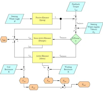
A custom algorithm was developed for use with the vehicle model (Equation 10) to determine the instantaneous
torque and power requirements for each component in a SBW package. A flowchart of this algorithm is shown in
Figure 33. First, the required torque is offset by the passive component torque (if one was used). Then the active
mechanical power required is calculated using the steering wheel angular velocity and the adjusted torque. If the
and the linear torque relationship (Equation 15). If the sign of the power is positive then the MR brake model (or
motor model depending on the design configuration) is used to determine the MR brake/motor current using the
MR brake/motor properties (Table 6). The total SBW torque is the sum of the passive, semi-active, and active
component torques. The electrical energy for each component is the time integral of the instantaneous electrical
power (Equation 16). Total electrical energy is the sum of the component electrical energies.
The computed SBW feedback torque (a summation of optimized component torques) was compared to the
measured vehicle steering torque by use of sum of squared errors (SSE) performance index:
n n
1 i
2
i sbw, τ i required, τ
PI
∑
=
− =
(19)
Where trequired,iis the recorded vehicle torque at time i, tsbw,i is the computed SBW torque at time i, and n is the total
number of samples. This comparison parameter was calculated for each speed, run, and SBW design.
3.3.1 Fully Passive
The steering feedback torque generated by a torsional spring is directly proportional to steering angle and therefore
cannot accurately produce the required torque profile, as shown in the representative torque vs. angular velocity plot
of Figure 32. Figure 34 shows the response vs. time for the same 48 kph run (and the optimized spring rate of
0.102 Nm/deg provided in Table 4.) Tables 8-10 summarize the performance of this SBW design option (and all
remaining design options) for all four runs at 48, 64, and 97 kph, respectively. Although this passive SBW design
does not fully model the expected torque input, it does reduce the torque remaining to be generated by the
0 5 10 15 -5
-4 -3 -2 -1 0 1 2 3 4 5
Time (sec)
T
o
rq
u
e
(N
m
)
Total Spring Total-Spring
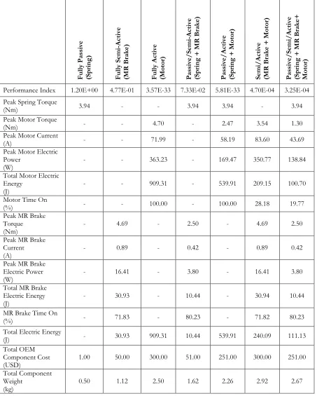
Table 8: Comparison of SBW design options and system performance at 48 kph F u ll y P a ss iv e (S p ri n g ) F u ll y S em i-A ct iv e (M R B ra k e ) F u ll y A ct iv e (M o to r) P a ss iv e/ S em i-A ct iv e (S p ri n g + M R B ra k e ) P a ss iv e/ A ct iv e (S p ri n g + M o to r) S em i/ A ct iv e (M R B ra k e + M o to r) P a ss iv e/ S em i/ A ct iv e (S p ri n g + M R B ra k e + M o to r)
Performance Index 1.20E+00 4.77E-01 3.57E-33 7.33E-02 5.81E-33 4.70E-04 3.25E-04 Peak Spring Torque
(Nm) 3.94 - - 3.94 3.94 - 3.94
Peak Motor Torque
(Nm) - - 4.70 - 2.47 3.54 1.30
Peak Motor Current
(A) - - 71.99 - 58.19 83.60 43.69
Peak Motor Electric Power
(W)
- - 363.23 - 169.47 350.77 138.84
Total Motor Electric Energy
(J)
- - 909.31 - 539.91 209.15 100.70
Motor Time On
(%) - - 100.00 - 100.00 28.18 19.77
Peak MR Brake Torque (Nm)
- 4.69 - 2.50 - 4.69 2.50
Peak MR Brake Current (A)
- 0.89 - 0.42 - 0.89 0.42
Peak MR Brake Electric Power (W)
- 16.41 - 3.80 - 16.41 3.80
Total MR Brake Electric Energy (J)
- 30.93 - 10.44 - 30.94 10.44
MR Brake Time On
(%) - 71.83 - 80.23 - 71.82 80.23
Total Electric Energy
(J) - 30.93 909.31 10.44 539.91 240.09 111.13
Total OEM Component Cost (USD)
1.00 50.00 300.00 51.00 251.00 300.00 251.00
Total Component Weight
(kg)
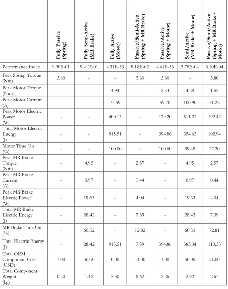
Table 9: Comparison of SBW design options and system performance at 64 kph F u ll y P a ss iv e (S p ri n g ) F u ll y S em i-A ct iv e (M R B ra k e ) F u ll y A ct iv e (M o to r) P a ss iv e/ S em i-A ct iv e (S p ri n g + M R B ra k e ) P a ss iv e/ A ct iv e (S p ri n g + M o to r) S em i/ A ct iv e (M R B ra k e + M o to r) P a ss iv e/ S em i/ A ct iv e (S p ri n g + M R B ra k e + M o to r)
Performance Index 9.90E-01 9.41E-01 4.31E-33 8.18E-02 4.61E-33 3.78E-04 3.10E-04 Peak Spring Torque
(Nm) 3.80 - - 3.80 3.80 - 3.80
Peak Motor Torque
(Nm) - - 4.94 - 2.53 4.28 1.52
Peak Motor Current
(A) - - 75.59 - 59.70 100.90 51.22
Peak Motor Electric Power
(W)
- - 400.13 - 179.20 511.21 192.42
Total Motor Electric Energy
(J)
- - 915.51 - 394.86 354.62 102.94
Motor Time On
(%) - - 100.00 - 100.00 39.48 27.20
Peak MR Brake Torque (Nm)
- 4.95 - 2.57 - 4.95 2.57
Peak MR Brake Current (A)
- 0.97 - 0.44 - 0.97 0.44
Peak MR Brake Electric Power (W)
- 19.63 - 4.04 - 19.63 4.04
Total MR Brake Electric Energy (J)
- 28.42 - 7.39 - 28.42 7.39
MR Brake Time On
(%) - 60.52 - 72.82 - 60.53 72.81
Total Electric Energy
(J) - 28.42 915.51 7.39 394.86 383.04 110.33
Total OEM Component Cost (USD)
1.00 50.00 0.00 51.00 1.00 50.00 51.00
Total Component Weight
(kg)