Standardized CUSUM Control Chart for Process Mean with MDSS

(1)

ISSN(Online): 2319-8753

ISSN (Print): 2347-6710

I

nternational

J

ournal of

I

nnovative

R

esearch in

S

cience,

E

ngineering and

T

echnology

(An ISO 3297: 2007 Certified Organization) Vol. 4, Issue 7, July 2015

Standardized CUSUM Control Chart for

Process Mean with MDSS

Pandurangan.A, Varadharajan.R

Department of Mathematics, SRM University, Kattankulathur, Chennai, Tamil Nadu, India

ABSTRACT: Many authors proposed the CUSUM control chart for single observation in each group (sample) to

detect even small shift in μ. In this paper a standardized CUSUM control chart is proposed for more than one observation in each sample. The variable sample size (VSS), and Markov dependent sample sizes (MDSS)of three types are considered to implement the standardized CUSUM control chart for process variability and illustrated in the tabular form.

KEYWORDS: Statistical Process Control(SPC), Cumulative Sum (CUSUM), Average Run Length(ARL), Variable Sample Size( VSS),Markov Dependent Sample Size(MDSS), Computer Simulation.

I. INTRODUCTION

Cumulative sum(CUSUM) control charts were first proposed by Page [6] and subsequently studied by many authors, like Arnold Jesse and Reynolds Marion[1]. The conventional Shewhart control chart may not give signal for smaller shifts in mean. The cumulative sum (CUSUM) control chart is a good alternative to identify the small shifts in μ and

to check the target process mean µ0[11,1,13].

The CUSUM is defined as:

S_i (X_i 



₀)S_i_₁; for i1, 2, 3,....with S₀0

In order to use the CUSUM

X

chart and check for any shift in mean, V-mask is used. But there are some disadvantages in developing a V-mask[12]. An alternative to this method is the tabular form. This can be easily implemented with the help of a computer.

II. A TABULAR FORM OF THE CUSUM

X

CONTROL CHARTS

Now a days it becomes a modern methodology to monitor the quality of product or process without drawing actual graphs. Montgomery[5], Pandurangan and Varadharajan[8] have proposed an algorithmic tabular CUSUM as well as standardized CUSUM to monitor the process mean[2]. Let SH(i) be an upper one sided tabular CUSUM for period i and

SL(i) be a lower one sided tabular CUSUM for sample i. Assuming X as iid normal with mean µ and variance

2



, the quantities

S

_H

(

i

)

and

S

_L

(

i

)

are defined for each sample as[3]

S

_H

(

i

)



Max

[

0 ,

X

_i



(



₀



K

)



S

_H

(

i



1 )]

and

(2)

ISSN(Online): 2319-8753

ISSN (Print): 2347-6710

I

nternational

J

ournal of

I

nnovative

R

esearch in

S

cience,

E

ngineering and

T

echnology

Starting with SH(0) or SL(0), when SHor SLbecomes negative reset to zero. If either SH(i) or SL(i) exceeds the decision

interval H[4,5], it must be concluded that the process is out of control. In that case the new process mean is estimated using the formula























H

i

S

if

N

i

S

K

H

i

S

if

N

i

S

K

H

L

)

(

)

(

)

(

)

(

)

(

)

(

1

0

0 ˆ



Where, the quantities NHand NLbe the number of consecutive periods that the CUSUMs SH(i) or SL(i) have been

non-zero[7].

The tabular CUSUM is designed by using the reference value of K and the decision interval H. It is usually recommended that these parameters are selected to provide a good run length value[6]. Montgomery[5] has

recommended K=0.5 and H= 4 or 5 to have a good ARL when the shift in the process mean is about 1σ[8].

III. FIRST INITIAL RESPONSE (OR) HEAD START

A procedure was introduced by Lucas and Crosier [4] to improve the sensitivity of a CUSUM at process start-up. Increased sensitivity at process start-up would be desirable if the corrective action did not reset the mean to the target value[10]. The first initial response (FIR) or head start essentially just sets the starting value

S

_H

(

0 )

and

S

_L

(

0 )

equal to non zero value typically H/2.

STANDARDIZED CUSUM

A drawback in the conventional CUSUM control chart is that the reference value of H and K must be chosen by satisfying certain conditions. To overcome this difficulty, instead of considering the actual average for each sample (sub group), it can be standardized as follows[9]:

(

0

)

;

i i

S

X

Z







for i = 1, 2, 3,……….

Where







n

i i

i

x

n

S

1 2

)

(

1

, (Si is the unbiased standard deviation for the ith sample)

Then the standardized CUSUM is calculated using

)]

1 (

,

0 [

)

(

i



Max

Z



K



S

i



S

_H _i _H

and

)]

1 (

,

0 [

)

(

i



Max

K



Z



S

i



S

_L _i _L

Then Zi becomes identically independently distributed standard normal variable[11].

(3)

ISSN(Online): 2319-8753

ISSN (Print): 2347-6710

I

nternational

J

ournal of

I

nnovative

R

esearch in

S

cience,

E

ngineering and

T

echnology

IV. NUMERICAL ILLUSTRATION

(i) Variable Sample Size (VSS)

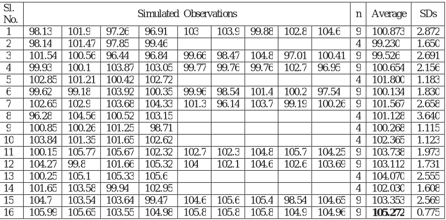
Charts with variable sample sizes can be used for certain advantages. Costa[3] has proposed a chart with variable sample sizes to study the process mean. The same concept is extended for CUSUM control chart. Consider a production process of forged piston rings with outer diameter (OD) as 100mm. The quality characteristics of the piston ring OD can be checked. In this case, the in–control production process is modeled as a normal process whose mean is equal to 100 mm with standard deviation 5 mm[13,5,7]. Box and Mullern[2] have suggested the method to simulate normal variable. Sample observations are simulated taking



= 100,



=5 for the first 10 samples (subgroups) and



= 101,



= 5 from 11th sample (subgroups) onwards. The sample sizes are taken as 9 or 4.

The Shewhart control limits for

X

chart with variable sample size are: UCL = 105.0; LCL = 95.0 for sample size n1 = 9 and

UCL = 107.5; LCL = 92.5 for sample size n2 = 4.

The simulated sample observations and subgroup averages are shown below.

Table 4

Sl.

No. Simulated Observations n Average SDs

1 98.13 101.9 97.26 96.91 103 103.9 99.88 102.8 104.6 9 100.873 2.872

2 98.14 101.47 97.85 99.46 4 99.230 1.650

3 101.54 100.56 96.44 96.84 99.66 98.47 104.8 97.01 100.41 9 99.526 2.691 4 99.93 100.1 103.87 103.05 99.77 99.76 99.76 102.7 96.95 9 100.654 2.156

5 102.85 101.21 100.42 102.72 4 101.800 1.183

6 99.62 99.18 103.92 100.35 99.96 98.54 101.4 100.2 97.54 9 100.134 1.830 7 102.65 102.9 103.68 104.33 101.3 96.14 103.7 99.19 100.26 9 101.567 2.658

8 96.28 104.56 100.52 103.15 4 101.128 3.640

9 100.85 100.26 101.25 98.71 4 100.268 1.115

10 103.84 101.35 101.65 102.62 4 102.365 1.123

11 100.15 105.77 105.67 102.32 102.7 102.3 104.8 105.7 104.25 9 103.738 1.973 12 104.27 99.8 101.66 105.32 104 102.1 104.6 102.6 103.69 9 103.112 1.731

13 100.25 105.1 105.33 105.6 4 104.070 2.555

14 101.65 103.58 99.94 102.95 4 102.030 1.608

15 104.7 103.54 103.64 99.47 104.6 105.6 105.4 98.54 104.65 9 103.353 2.569 16 105.99 105.65 103.55 104.98 105.8 105.8 105.8 104.9 104.96 9 105.272 0.775

The simulated inspection is terminated since the average goes beyond the UCL of the conventional Control Chart. By using the subgroup averages

X

_i the standardized CUSUM for each sample is calculated. For example, the

initial values are:

S

_H

(

0 )



0 

S

_L

(

0 )

0 .

303751

871501

.

12

100 8722

.

100 )

(

1 0 1

1











S

X

(4)

ISSN(Online): 2319-8753

ISSN (Print): 2347-6710

I

nternational

J

ournal of

I

nnovative

R

esearch in

S

cience,

E

ngineering and

T

echnology

and

S

_L

(

1 )



Max

[

0 ,

0 .

5 

Z

₁



S

_L

(

0 )]



Max

[

0 ,

0 .

5 

0 .

303751



0 ]



0 .

196249

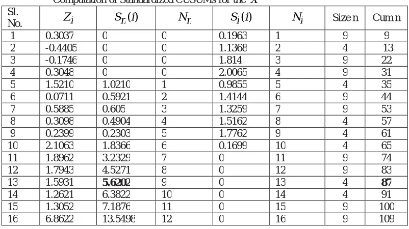
And so on. The computations are given in the Table 5 below:

Table 5

Computation of Standardized CUSUMs for the X

Sl.

No. Zi Sn(i) Nn Si(i) Ni Size n Cum n

1 0.3037 0 0 0.1963 1 9 9

2 -0.4405 0 0 1.1368 2 4 13

3 -0.1746 0 0 1.814 3 9 22

4 0.3048 0 0 2.0065 4 9 31

5 1.5210 1.0210 1 0.9855 5 4 35

6 0.0711 0.5921 2 1.4144 6 9 44

7 0.5885 0.605 3 1.3259 7 9 53

8 0.3098 0.4904 4 1.5162 8 4 57

9 0.2399 0.2303 5 1.7762 9 4 61

10 2.1063 1.8366 6 0.1699 10 4 65

11 1.8962 3.2329 7 0 11 9 74

12 1.7943 4.5271 8 0 12 9 83

13 1.5931 5.6202 9 0 13 4 87

14 1.2621 6.3822 10 0 14 4 91

15 1.3052 7.1876 11 0 15 9 100

16 6.8622 13.5498 12 0 16 9 109

The standardized CUSUM for X from the above Table 5 indicates that the process is out of control at sample 13 since SHis greater than 5.

Now we form the standardized CUSUM with the first initial value SH(0) = 2.5 = SL(0).

The computations are as follows:

SH(1) = Max[0, Z1-0.5 + SH(0)] = Max[0, 0.303751-0.5+2.5]=2.3038

SL(1) = Max[0, 0.5-Z1 + SL(0)] = Max[0, 0.5-0.303751+2.5]=2.6962

SH(2) = Max[0, Z2-0.5 + SH(1)] = Max[0, 0.440525-0.5+2.3038]=1.3632

SL(2) = Max[0, 0.5-Z2 + SL(1)] = Max[0, 0.5-(-0.440525)+2.6962]=3.66377

(5)

ISSN(Online): 2319-8753

ISSN (Print): 2347-6710

I

nternational

J

ournal of

I

nnovative

R

esearch in

S

cience,

E

ngineering and

T

echnology

The standardized CUSUM chart in the above table indicates the process is out of control at sample 12, since SHis greater than 5 the total sample inspection is only 83 when head start is H/2. The standardized CUSUM control

chart with variable sample size(VSS) takes 87 sample observations to signal when the initial value is 0.

(ii) Markov Dependent Sample Size

Markov chain rule plays an important role in sample selection. Pandurangan[7] has suggested various control charts under Markovian environment. Consider the illustration given in his work for Markov Dependent Sample Size (MDSS). The specified outer diameter (OD) of the piston rings was taken as 100 mm. In this case, the in-control production process whose mean is equal to 100mm with standard deviation 5 mm. To check the quality, sample observations were simulated for each subgroup of size 6 or 4 or 5.[7,5,7] The size of each subgroup is decided on Markov Chain rule.

To decide the size of an MDSS, the TPM was taken with weights 8, 7 and 5 respectively for the sample sizes 6,4 and 5.















5 /

1

5 /

3

5 /

1

7 /

2

7 /

2

7 /

3

8 /

2

8 /

3

8 /

3

(6)

ISSN(Online): 2319-8753

ISSN (Print): 2347-6710

I

nternational

J

ournal of

I

nnovative

R

esearch in

S

cience,

E

ngineering and

T

echnology

By a random technique (lottery method) an MDSS sequence is obtained as:

1 

3 

1 

3 

2 

1 

2 

3 

1 

3 

1 

2 

1

Where 1 denotes type-1 sample of size n1 = 6, 2 denotes type-2 sample of size n2 = 4 and 3 denotes type-3 sample of

size n3=5. Then the control limits for chart under MDSS are:

104 .

0411

3

2

3

2

1

2

1

0

3

0 





n

UCL







95 .

9589

3

2

3

2

1

2

1

0

3

0 





n

LCL







Sample observations were simulated with



= 100 mm and



= 5 mm for the first 10 samples and then



= 101 mm and



= 5 mm from the 11th sample onwards. The subgroup averages are shown in Table 7.

Table-7

The above table has issued an alarm at the 15th subgroup, since the mean value exceeds the UCL with n = 6. But actually the shift has occurred at the 11th sample. Total items inspected was 78.

By using

X

_ia tabular CUSUM is formed by standardizing the variable.

Then the calculation of SH(i) and SL(i) are as follows. The first initial value SH(0) = 0, SL(0) = 0 to be used

S.No n Mean SDs

1 101.35 98.50 100.85 99.65 103.00 103.92 6 101.212 2.024 2 100.35 102.45 102.85 101.65 100.55 5 101.570 1.112 3 100.25 98.85 99.85 100.20 99.66 100.35 6 99.860 0.560 4 102.05 100.25 103.87 103.05 99.77 5 101.798 1.763 5 102.85 98.20 100.42 99.15 4 100.155 2.014 6 100.55 99.18 98.48 102.42 99.96 99.16 6 99.958 1.403 7 102.35 102.90 99.58 104.33 101.25 99.14 6 101.592 1.998

8 101.45 98.54 100.52 99.15 4 99.915 1.316

9 101.52 100.26 102.32 102.71 101.25 5 101.612 0.958 10 100.15 101.66 99.45 98.25 102.65 100.25 6 100.402 1.566 11 104.27 102.25 103.66 104.33 104.55 5 103.812 0.933 12 102.85 105.45 103.65 103.40 102.85 103.65 6 103.642 0.957 13 103.25 104.35 105.65 102.38 4 103.908 1.414 14 104.17 104.32 104.35 102.85 4 103.923 0.719 15 105.92 104.94 105.40 105.20 104.35 105.65 6 105.243 0.555

(7)

ISSN(Online): 2319-8753

ISSN (Print): 2347-6710

I

nternational

J

ournal of

I

nnovative

R

esearch in

S

cience,

E

ngineering and

T

echnology

5988

.

0

024 .

2

100

212 .

101 )

(

1 0 1

1











S

X

Z



SH(1) = Max[0,Z1-0.5 + SH(0)]=Max[0,0.5988 - 0.5+0]=0.0988

SL(1) = Max[0,0.5-Z1 + SL(0)]=Max[0,0.5-0.5988+0]=0

SH(2) = Max[0,Z2-0.5 + SH(1)]=Max[0,1.4119-0.5+0.0988]=1.0107

SL(2) = Max[0,0.5-Z2 + SL(1)]=Max[0,0.5-(1.4119)+0]=0

And so on. The computations are given in the following Table 8.

Table-8

The above Table 8 indicates the process is out of control at sample 12, since SH is greater than 5. But in the case of

conventional MDSS control chart a signal was obtained in the 15th sample. The sample inspection in this case is 64 whereas it was 78 in the case of conventional MDSS system. Thus, the standardized CUSUM control chart system for average is more economical than the conventional Shewhart control chart for VSS or MDSS.

V. CONCLUSION

The Standardized CUSUM control chart is used to monitor the process mean. The Standardized CUSUM system can easily identify even a small shift in the process mean. This method is compared with the conventional Shewhart control chart for Fixed Sample Size (FSS), Variable Sample Size (VSS) and Markov Dependent Sample Size (MDSS). Among all the three methods, the Standardized CUSUM control chart with MDSS proposed in this paper is shown to be the most economical chart. This procedure can be extended to detect the small shift in the process mean by using the sample median.

S.No. Zi SH(i) NH SL(i) NL n cum n

1 0.5988 0.0988 1 0 0 6 6

2 1.4116 1.0104 2 0 0 5 11

3 -0.2500 0.2604 3 0.750 1 6 17

4 1.0198 0.7802 4 0.230 2 5 22

5 0.0770 0.3572 5 0.653 3 4 26

6 -0.0297 0.0 0 1.183 4 6 32

7 0.7966 0.2966 1 0.886 5 6 38

8 -0.0646 0.0 0 1.451 6 4 42

9 1.6819 1.1819 1 0.269 7 5 47

10 0.2565 0.9384 2 0.512 8 6 53

11 4.0836 4.5220 3 0 0 5 58

12 3.8041 7.8261 4 0 0 6 64

13 2.7636 10.0897 5 0 0 4 68

14 5.4530 15.0427 6 0 0 4 72

(8)

ISSN(Online): 2319-8753

ISSN (Print): 2347-6710

I

nternational

J

ournal of

I

nnovative

R

esearch in

S

cience,

E

ngineering and

T

echnology

REFERENCES

[1].Arnold Jesse C., and Reynolds Marion R. Jr., “CUSUM Control with Sample Size and Sampling Intervals”, Journal of Quality Technology,

33(1), pp. 66-81.(2001)

[2]Jayaraman B., Valiathan G.M., Jayakumar K., Palaniyandi A., Thenumgal S.J., Ramanathan A., "Lack of mutation in p53 and H-ras genes in phenytoin induced gingival overgrowth suggests its non cancerous nature", Asian Pacific journal of cancer prevention : APJCP, ISSN : 13(11) (2012) PP. 5535-5538.

[3].Box, and M. E. Mullerm “A Note on the Generation of Random Normal Deviates”, Ann. Math. Statistics, 29, pp. 610-611. (1958)

[4].Kalaiselvi V.S., Saikumar P., Prabhu K., Prashanth Krishna G., "The anti Mullerian hormone-a novel marker for assessing the ovarian reserve in women with regular menstrual cycles", Journal of Clinical and Diagnostic Research, ISSN : 0973 - 709X, 6(10) (2012) PP.1636-1639.

[5].Costa A. F. B., “Chart with Variable Sample Size”, Journal of Quality Technology, 26, pp.155-163. (1994)

[6].Subhashree A.R., Shanthi B., Parameaswari P.J., "The Red Cell Distribution Width as a sensitive biomarker for assessing the pulmonary function in automobile welders- a cross sectional study", Journal of Clinical and Diagnostic Research, ISSN : 0973 - 709X, 7(1) (2013) PP. 89-92.

[7].Lucas J. M., and Crosier R. B., “Fast Initial Response for CUSUM Quality Control Schemes”, Technometrics, 24, (1982).

[8].Gopalakrishnan K., Prem Jeya Kumar M., Sundeep Aanand J., Udayakumar R., "Analysis of static and dynamic load on hydrostatic bearing with variable viscosity and pressure", Indian Journal of Science and Technology, ISSN : 0974-6846, 6(S6) (2013) PP.4783-4788.

[9]. Montgomery D.C. Introduction to Statistical Quality Control, 5th_{Edn. John Wiley and Sons, New York. 2005.}

[10].Srinivasan V., "Analysis of static and dynamic load on hydrostatic bearing with variable viscosity and pressure", Indian Journal of Science and Technology, ISSN : 0974-6846, 6(S6) (2013) PP.4777-4782.

[11]. Page. E.S “Cumulative Sum Control Charts,” Technometrics, Vol 3, pp. 1-9. (1961)

[12]. Pandurangan A., “Some Applications of Markov Dependent Sampling Scheme in SQC”, Unpublished Ph.D Thesis, Bharathidasan University, Tiruchirappalli, (2002).