On Designing Skip- Lot Sampling System

On Designing Skip- Lot Sampling System

M.Saranya

, Dr.S.Muthulakshmi

Research Scholar, Department of Mathematics, Avinashilingam Institute for Home Science and Higher Education for

Women, Coimbatore, Tamil Nadu, India1

Professor, Department of Mathematics, Avinashilingam Institute for Home Science and Higher Education for Women,

Coimbatore , Tamil Nadu, India2

ABSTRACT: This paper deals with designing of a new skip-lot sampling system having two different reference sampling plans with same sample size and two different acceptance numbers. The operating procedure of the new system and the derivation of performance measures using Markov-chain formulation are given. The designing of the system for two specified points on the OC curve and AOQL of the developed plan are given. The effect of system parameters on the performance measures are evaluated. The efficiency of the proposed sampling system is illustrated with matched SkSP-2 and single sampling plans.

KEYWORDS: Acceptable quality level, Average sample number, Single sampling plan, Skip-lot sampling system, Operating characteristic function.

I. INTRODUCTION

The acceptance sampling plans have been widely used in industries for maintaining the high quality level of the product at the minimum inspection cost. The skip-lot sampling schemes, have the provision of inspecting only a fraction of lots. Dodge [5] introduced SkSP-1 plan in chemical and physical processes to reduce inspection cost as an extension of continuous sampling plan, CSP-1 of Dodge [4]. Perry [8] proposed skip-lot sampling plan of type SkSP-2 by using single sampling plan as the reference plan and discussed the applications of the plan. Brugger [3] provided the derivation measures by employing simplified Markov-chain approach for SkSP-2 plan. Perry [9] extended the single level SkSP-2 plan to two levels of skipping inspection and derived their performance measures.

Vijayaraghavan [12] extended the SkSP-2 beyond two levels of sampling and using a general non-cost based approach to design skip-lot sampling plans and obtained tables using Poisson model. Govindaraju [7] studied the properties of SkSP-2 plan using single sampling plan with zero acceptance number as the reference plan. Balamurali et.al [2] proposed SkSP-R plan by including resampling and provided their performance measures. Aslam et.al [1] proposed SkSP-2 plan with two-stage group acceptance sampling plan as reference plan.

II. RELATED WORK

Stephens and Larson [11] indicated that an acceptance sampling system consisting of two or more sampling inspection plans and the rules for switching between them to achieve blending of the advantageous features of each of the sampling plans. This motivated the researcher to design the general skip-lot sampling system with two different reference sampling plans as a generalization of SkSP-2. In this paper a new skip-lot sampling system having two different reference sampling plans with same sample sizes and different acceptance numbers is introduced.

III. OPERATING PROCEDURE OF THE SYSTEM

The operating procedure of general skip-lot sampling system (GSkSS) has the following steps.

1. Start with normal inspection, using the reference sampling plan, rN. At this stage every lot is inspected. 2. When i consecutive lots are accepted on normal inspection, switch to skipping inspection at rate f, using the

reference sampling plan rS.

3. When a lot is rejected, switch to normal inspection. Screen each rejected lot and replace all nonconforming units found.

This new system designated as GSkSS (i, f, n, cN, cS) – refers to a skip-lot sampling system where the normal and skipping single sampling plans have the same sample size n, but different acceptance numbers cN and cS with cN ≤ cS. where cN is the acceptance number for normal inspection reference plan, rN and cS is the acceptance number for skipping inspection reference plan,rS. If cN = cS the system degenerates into a skip-lot sampling plan of type SkSP-2 with parameters (i,f,n,c).

IV. MEASURES OF PERFORMANCE

The performance measures are derived using Markov-Chain approach due to Robert’s [10]. The states of GSkSS are defined as

NO - Lot rejected on normal inspection using reference plan rN.

NJ - j lots are consecutively accepted during normal inspection using reference plan rN, j = 1, 2, ……..,i

SA - lot is accepted during skipping inspection at rate f, using reference plan rS. SR - lot is rejected during skipping inspection at rate f, using reference plan rS. SN - lot is skipped during skipping inspection at rate f, using reference plan rS.

The one-step transition matrix for the GSkSS plan is presented in Table A

TABLE-A TRANSITION PROBABILITY MATRIX OF GSkSS

State at tth trial

Sta

te

a

t

(t

-1)

st t

ria

l

N0 N1 N2 … Ni SA SR SN

N0 Q P • • • • •

N1 Q • P • • • •

• • •

•

Ni-1 Q • • P • • •

Ni • • • • fP1 fQ1 (1-f)

SA • • • • fP1 fQ1 (1-f)

SR Q P • • • • •

SN • • • • fP1 fQ1 (1-f)

In the matrix,

P - the probability of acceptance of a lot according to reference plan rN

P1 - the probability of acceptance of a lot according to reference plan rS Q1 - 1 –P1

Using thistransition probability matrix, the steady state probabilities j satisfy the following conditions



j ≥ 0 for all (i+4) states and







4

1

i

j j



are derived as

N0 = (1–P

i

) fQQ1 / D

N1 = fQQ1P / D

Nj = fQQ1P/D, j = 2, 3, ……..,i (1)

SA = fQP1Pi / D

SR = fQQ1Pi / D

SN = (1–f)QP i

/ D, where D = fQ1 +P i

(Q–fQ1)

The operating characteristic function of GSkSS is Pa = 1 – SR – NO

= {fQ1P + P i

(Q – fQ1)} / D (2)

The average fraction of total lots inspected (AFI) comprised of lots from normal inspection and a fraction, f of the lots during skipping inspection. Therefore,

F = 1 – SN

= {fQ1(1–Pi) + fQPi} / D (3)

A very important property of skip-lot sampling scheme is that of reduced inspection, it will be investigated with the help of average sample numbers ASN (GSkSS) = F•ASN(R), where ASN(R) is the average sample number of units inspected per lot under normal and skipping inspection.

ASN(R) = n

V. MATHEMATICAL PROPERTIES OF Pa

The mathematical properties and relationships between Pa and each of its parameters – i, f, P and P1 are investigated. The results obtained will hold for all values of i and f.

i) Pa = 1 – [Q1(1 – P) / {Pi Q / f + Q1(1 – Pi)}]

implies Pa is a increasing function of f (i, P, P1 are fixed) ii) Pa = 1 – [{f Q1 Q} / {f Q1 + Pi(Q – fQ1) }]

implies Pa is a decreasing function of i (f, P, P1 are fixed) iii) Pa = P[Q1 + Pi-1(Q – fQ1)] / [fQ1 + Pi (Q – fQ1)]

implies Pa≥ P and Pa ≥ P1,since Pi < Pi-1

iv) Pa is a increasing function of P as well as P1 (i, f are fixed)

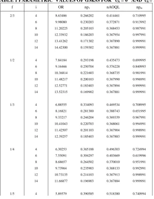
VI. DESIGNING OF SYSTEM FOR GIVEN TWO FIXED POINTS ON THE OC CURVE(P1,1-α), (P2,β)

Tables 1 and 2 may be used to design GSkSS with two reference single sampling plans having two different acceptance numbers but same sample size for a given p1, p2, α and β. Consider the designing of GSkSS for the given p1 = 0.006, p2 = 0.04, α = 0.05 and β = 0.10.

Compute the operating ratio, OR = p2/p1 = 6.66.

From Table 1 one obtains OR=6.8855. The associated np1 is 0.334093, therefore the sample size for normal and skipping reference plans is n = np1 / p1~ 56. Thus the required GSkSS (i, f, n, cN, cS) is (4, 1/3, 56, 0, 1).

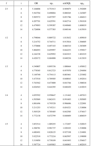
From Table 2 one obtains OR=6.7260. The associated np1 is 0.577383, which gives the sample size as n=96. Thus the required GSkSS (i, f, n, cN, cS) is (14, 2/3, 96, 1, 2).

VII. CALCULATION OF AOQL OF A GIVEN PLAN

Table 2 may be used to calculate AOQL and pm of given system. For example one requires AOQL for a given system with n=56, f=2/3, i=14, cN =1 and cS =2. Table 2 gives nAOQL =0.840146 and npm = 1.615019. Therefore AOQL= 0.015002 and pm= 0.028839. This indicates that the worst outgoing quality of using the plan GSkSS (14,2/3,56,1,2) is 0.028839 for any incoming lot quality.

VIII. EFFECT OF PARAMETERS i AND f ON PERFORMANCE MEASURES

The effect of i and f on probability of acceptance and average fraction of lots inspected are illustrated graphically. Probability of acceptance curves for fixed i and fixed f are presented in fig.1 and the corresponding AFI curves are presented in fig.2. Figures reveal that i) For a fixed i, increase in f increases OC value when the quality is good and increases AFI irrespective of the incoming quality ii) For a fixed f, increse in i decreases OC value when the quality is poor and increases AFI.

Fig-1 OC curves for same i different f OC curves for same f different i

Fig-2 AFI curves for same i different f AFI curves for same f different i

0 0.2 0.4 0.6 0.8 1 1.2

0 0.02 0.04 0.06

GSKSS(4,1/ 4,100,1,2) GSKSS(4,2/ 3,100,1,2)

0 0.2 0.4 0.6 0.8 1 1.2

0 0.02 0.04 0.06

GSKSS(4,1/4,1 00,1,2) GSKSS(10,1/4, 100,1,2)

0 0.2 0.4 0.6 0.8 1 1.2

0 0.02 0.04 0.06

GSKSS(4,1/ 2,100,1,2) GSKSS(4,1/ 3,100,1,2)

0 0.2 0.4 0.6 0.8 1 1.2

0 0.02 0.04 0.06

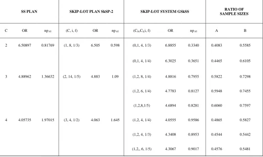
IX. COMPARISON OF GSKSS WITH SKSP-2 AND SS PLANS

Grubbs [6] suggested a measure to compare, called "Operating Ratio" which is defined as p0.10/p0.95 where p0.10 and p0.95 are the values of p with Pa = 0.10 and 0.95 respectively. This reflects the ability of a plan to discriminate between good and bad quality. The matched GSkSS, SkSP-2 and SS plans are obtained by means of nearly equal OR values.

Some GSkSS and reasonably well-matched SkSP-2 plans and single sampling plans are given in Table 3 Suppose that one requires a plan for p1 = 0.015 p2 = 0.072, α = 0.05, and β = 0.10. The operating ratio is 4.8. From Table 3

I) The SSP with n = 91, c = 3, np1 is 1.3663

ii) The SkSP-2 plan with i = 14, f = 1/5, n = 73, c = 2, np1 is 1.09 iii) GSkSS with f = 1/4/, i = 6, n = 54, cN = 1, cS = 2, np1 is 0.8127 iv) GSkSS with f = 1/4, i = 8, n = 54,cN =1, cS = 2 and np1 is 0.7955

Further, the last two columns in table 3 when subtracted from 1.0 represent the percent reduction in the sample size of GSkSS with that of SkSP-2 and SS matched plans. This shows reduction in sample size for GSkSS over SkSP-2 plan and single sampling plan. This suggests the economy of the proposed plan.

X. CONCLUSION

A new skip-lot sampling system called GSkSS has been proposed in this paper. The two points on the OC curve approach is adopted to design parameters of the proposed system. Various measures of performance for proposed system have been derived using Markov chain model. The proposed system is found to be more efficient than the matched single and SkSP-2 plans. It is found that the proposed system requires the less number of sample units for the inspection purpose than the conventional single and SkSP-2 plans. So the proposed system is useful in reducing the cost and the time of inspection of the material or the product.

XI. CONSTRUCTION OF TABLES

The OC function of GSkSS derived in (2) is

Pa = {Fq1 P + Pi(Q – Fq1)} / {Fq1 + Pi(Q – Fq1)} (4) Under Poisson model with single sampling reference plans,

P = exp(-np) (np)d /d! (5)

P = exp(-np) (np)d /d! ₍₆₎

when we use the reference sampling plans with different acceptance numbers and same sample size. Now for assumed values of i, f and Pa(p) (in equation 2) can be solved for np by the methods of successive approximation.

First and second columns of Tables 1 and 2 the values relating to operating ratio and np1 corresponding to α = 0.05 and β = 0.10 are obtained and furnished.

Assuming nAOQ = np.Pa(P), values of npmthat maximizes Naoq are obtained by the method of iterations and the nAOQL values are obtained as nAOQLm= npm.Pa(pm). The values of npm and nAOQL are provided in third and fourth columns of Tables 1 and 2. The tables are constructed by assuming cN (= 0,1),cS (= 1,2), i ( = 4, 6, 8, 10, 12, 14) and f (= 2/3, 1/2, 1/3,1/4, 1/5).

C+1

c

d=0

REFERENCES

[1]. Aslam, M. et.al ., ”Skip-Lot Sampling Plan of Type SkSP-2 with Two-Stage Group Acceptance as Reference Plan”, Communications in Statiatics-Simulation and Computation., pp. 777-789, 2015

[2]. Balamurali S., et.al, “A New System of Skip-Lot Sampling Plans including Resampling”, The scientific world journal, 5(2) pp. 1-6, 2014

[3]. Brugger, R.M., “A Simplification of Skip-Lot Procedure Formulation”, Journal of Quality Technology, 7 (4), pp. 165-167, 1975.

[4]. Dodge, H.F., “A Sampling Inspection Plan for Continuous Production”, Annals of Mathematical Statistics, 14, pp. 264- 279,1943.

[5]. Dodge, H.F., “Skip-Lot Sampling Plan Industrial Quality Control”, 11(5), pp. 3-5, 1955.

[6]. Grubbs, F.E.,"On Designing Single Sampling Inspection Plan", Annals of Mathematical Statistics, 20, pp. 242-256, 1949.

[7]. Govindaraju, K.,,”Contributions to the Study of Certain Special Purpose plans”, Ph.D. Thesis, Bharathiar University, Coimbatore, TamilNadu, India,1994.

[8]. Perry, R.L., “Skip-Lot Sampling Plans”, Journal of Quality Technology, 5 (3), pp. 123-130, 1973a,.

[9]. Perry, R.L., “Two-Level Skip-Lot Sampling Plans, Operating Characteristic Properties, Journal of Quality Technology, 5 (4), pp. 160-166,1973b.

[10]. Roberts., S., “Statesof Markov Chains for Evaluating Continuous Sampling Plans”, Transactions of the 17th _{Annual All Day Conference}

on Quality Control, Metropolitan Section, ASQC and Rutgers University, New Brunswick, N.J., pp. 106-111, 1965.

[11]. Stephens., K.S., and Larson, K.E, “An Evaluation of the MIL-STD-105D System of Sampling Plans”, Introduction to Quality Control, 23 (7), pp. 310-319, 1967.

[12]. Vijayaraghavan, R., “Contributions to the Study of Certain Sampling Inspection Plans by Attributes”, Ph.D. Thesis, Bharathiar University, Coimbatore, Tamil Nadu, India,1990.

TABLE 1 PARAMETRIC VALUES OF GSkSS FOR cN = 0 AND cS = 1

f i OR np1 nAOQL npm

2/3 4 8.63486 0.266202 0.414461 0.710995

6 9.98080 0.230203 0.372871 0.913992

8 11.20225 0.205103 0.368453 0.987991

10 12.33932 0.186203 0.367954 0.997991

12 13.41262 0.171302 0.367890 0.999991

14 14.42300 0.159302 0.367881 0.999991

1/2 4 7.84184 0.293198 0.435473 0.699995

6 9.16466 0.250704 0.376228 0.840993

8 10.36814 0.221603 0.368735 0.981991

10 11.48217 0.200103 0.367990 0.996991

12 12.52771 0.183403 0.367894 0.999991

14 13.52315 0.169902 0.367881 0.999991

1/3 4 6.88555 0.334093 0.469534 0.708995

6 8.16821 0.281300 0.388743 0.651995

8 9.33217 0.246204 0.369339 0.967991

10 10.41043 0.220703 0.368061 0.994991

12 11.42507 0.201103 0.367904 0.998991

14 12.39257 0.185403 0.367883 0.999991

1/4 4 6.30253 0.365188 0.496303 0.724994

6 7.55091 0.304297 0.403669 0.619996

8 8.68657 0.264502 0.370010 0.951991

10 9.73964 0.235903 0.368133 0.992991

12 10.73135 0.214103 0.367913 0.998991

14 11.66877 0.196903 0.367884 0.999991

6 7.11600 0.322894 0.417046 0.613996

8 8.22928 0.279200 0.370775 0.929992

10 9.26070 0.248104 0.368206 0.990991

12 10.23421 0.224503 0.367922 0.998991

14 11.15331 0.206003 0.367885 0.999991

TABLE 2 PARAMETRIC VALUES OF GSkSS FOR cN = 1 AND cS = 2

f i OR np1 nAOQL npm

2/3 4 5.166006 0.751913 0.969879 1.392009

6 5.563704 0.698004 0.888365 1.343007

8 5.905572 0.657597 0.851786 1.484013

10 6.207701 0.625591 0.842714 1.581018

12 6.479093 0.599387 0.840660 1.606019

14 6.726006 0.577383 0.840146 1.615019

1/2 4 4.798046 0.809722 1.013632 1.409010

6 5.214752 0.744711 0.913816 1.306005

8 5.570888 0.697103 0.860310 1.383009

10 5.884093 0.659997 0.844253 1.559017

12 6.164338 0.629992 0.841015 1.601019

14 6.420172 0.604888 0.840236 1.613019

1/3 4 4.340807 0.895336 1.080664 1.450012

6 4.778365 0.812723 0.957070 1.294004

8 5.149740 0.754113 0.883461 1.253002

10 5.473510 0.709505 0.848043 1.492014

12 5.763562 0.673800 0.841766 1.588018

14 6.026563 0.644395 0.840420 1.610019

1/4 4 4.055592 0.958647 1.131462 1.487013

6 4.503069 0.862431 0.991603 1.305005

8 4.881696 0.795520 0.906686 1.222001

10 5.211253 0.745211 0.854321 1.318006

12 5.505329 0.705405 0.842585 1.574017

14 5.772130 0.672799 0.840609 1.606019

1/5 4 3.853514 1.009255 1.172497 1.520015

6 4.306781 0.901737 1.020102 1.318006

8 4.689491 0.828125 0.927198 1.216001

10 5.022510 0.773216 0.865997 1.198000

12 5.319050 0.730109 0.843493 1.556017

TABLE 3 COMPARISON OF SAMPLE SIZES - GSkSS WITH SkSP-2 AND SSP

A = RATIO OF SAMPLE SIZES OF GSkSS WITH SS PLAN

B = RATIO OF SAMPLE SIZES OF GSkSS WITH SkSP-2 PLAN

SS PLAN SKIP-LOT PLAN SkSP-2 SKIP-LOT SYSTEM GSkSS RATIO OF SAMPLE SIZES

C OR np.95 (C, i, f) OR np.95 (CN,CS,i, f) OR np.95 A B

2 6.50897 0.81769 (1, 8, 1/3) 6.505 0.598 (0,1, 4, 1/3) 6.8855 0.3340 0.4083 0.5585

(0,1, 4, 1/4) 6.3025 0.3651 0.4465 0.6105

3 4.88962 1.36632 (2, 14, 1/5) 4.883 1.09 (1,2, 8, 1/4) 4.8816 0.7955 0.5822 0.7298

(1,2, 6, 1/4) 4.7783 0.8127 0.5948 0.7455

(1,2,8,1/5) 4.6894 0.8281 0.6060 0.7597

4 4.05735 1.97015 (3, 4, 1/2) 4.063 1.645 (1,2, 4, 1/4) 4.0555 0.9586 0.4865 0.5827

(1,2, 4, 1/3) 4.3408 0.8953 0.4544 0.5442