Response to perturbations for granular flow in a hopper
John F. Wambaugh
National Center for Computational Toxicology, US EPA, Research Triangle Park, NC 27711 and
Department of Physics and Center for Nonlinear and Complex Systems, Duke University, Durham, NC 27708∗
John V. Matthews
Department of Mathematics, University of Tennessee at Chattanooga, Chattanooga, TN 37403
Pierre A. Gremaud
Department of Mathematics and Center for Research in Scientific Computation, North Carolina State University, Raleigh NC, 27695-8205
Robert P. Behringer
Department of Physics and Center for Nonlinear and Complex Systems, Duke University, Durham, NC 27708∗
Abstract
We experimentally investigate the response to perturbations of circular symmetry for dense
granular flow inside a three-dimensional right-conical hopper. These experiments consist of
par-ticle tracking velocimetry for the flow at the outer boundary of the hopper. We are able to test
commonly used constitutive relations and observe new granular flow phenomena that we can model
numerically. Unperturbed conical hopper flow has been described as a radial velocity field with
no azimuthal component. Guided by numerical models based upon continuum descriptions, we
find experimental evidence for secondary, azimuthal circulation in response to perturbation by
tilting. For small perturbations we can discriminate between constitutive relations, based upon
the agreement between the numerical predictions they produce and our experimental results. We
find that the secondary circulation can be suppressed as wall friction is varied, also in agreement
with numerical predictions. For large tilt angles we observe the abrupt onset of circulation for
parameters where circulation was previously suppressed. Finally, we observe that for large tilt
angles the fluctuations in velocity grow, independently of the onset of circulation.
PACS numbers:
I. INTRODUCTION
Many practical processes involve the flow of dense granular materials. Applications range from food grains, ores, and coal to pharmaceutical powders. To predict flows of dense granular states, one would like a homogenized/continuum model that reflects the complexity of grain-scale interactions but can be applied at much larger scales. Continuum approaches frequently describe granular materials using elasto-plastic models in which the material can support shear stresses up to a certain value before yielding and deforming irreversibly. In the simplest case, this approach amounts to Coulomb’s law of friction.
The most common yield criterion is the Mohr-Coulomb criterion, which proposes a linear relationship between the magnitudes of normal stressσand shear stressτ in two-dimensions. Because the choice of axes dictates the relative magnitude of the normal and shear stresses, the range of possible axes maps out a circle in the space of normal and shear stress — the “Mohr circle”. The diameter of this circle is proportional to the magnitude of the stresses [1].
In the normal-shear stress space, the Mohr-Coulomb yield criterion is the straight line τ = µσ + c where µ is the coefficient of friction and c is the cohesion. It follows for cohesionless granular materials, the case we consider here, that the yield criterion must pass through the origin. The stress within the material, and hence the diameter of the Mohr circle, can increase only until the yield criterion is tangent to the circle. The point of contact then indicates an axis of a coordinate frame in which the ratio of shear to normal stress (equivalent to the mobilization of friction) is maximized. In this two-dimensional analysis of a three-dimensional material, the direction of the maximally mobilized shear stress and the third, neglected, axis span the “mobilized plane” along which motion of the granular material is most likely in response to stress [1].
Unfortunately, the mathematics of continuum descriptions of granular materials are rife with instatbilities, ill-posedness, and complex non-linearities [4]. This means that evaluating the response of granular materials to perturbations that cause unusual behavior in continuum models is necessary to determine the physical relevance of such approaches.
The right-conical hopper provides an ideal test system for granular flow in that it is not only an experimentally-accessible system, but also because the behavior is commonly as-sumed to tend to a steady-state with known velocity and stress field solutions derived from soil mechanics. The so-called Jenike radial solutions describe the velocity and stress fields in an infinite hopper as self-similar functions of radial position alone, without non-radial ve-locity components [5]. In two dimensions, such soil mechanics descriptions of wedge hoppers have been studied extensively both experimentally [6–9] and theoretically [10, 11]. Three-dimensional, right-conical hopper flow has been studied through experiments and discrete element simulations in the past[12, 13], but these studies did not make direct comparision to soil mechanics predictions.
Recent numerical work has taken advantage of the self-similar nature of the solution even in relatively general three-dimensional geometries such as “pyramidal” hoppers. By perturb-ing the geometry of the simulated hopper, the response of the continuum description can be examined. In particular, numerical work has found that secondary, non-radial circulation currents arise. These currents depend sharply upon model parameters in non-trivial ways [14–16].
II. SOIL MECHANICS APPROACHES TO GRANULAR MATTER
Before turning to the experiments, we give a brief summary of the relevant soil mechanics consitutive relations. At issue are the determining equations for the stress tensor. Force balance gives six equations for the nine components of the three dimensional stress tensor. To close this system of equations we need additional constitutive relations describing the yielding, plasticity and flow of the material [15]. Consideration of the velocity fieldv describ-ing the flow introduces three more unknowns brdescrib-ingdescrib-ing the necessary number of additional constraint equations to six.
We use Levy’s flow rule to introduce five constraints [1, 17]. Missing is a final constitutive relation describing the stress sufficient to cause plastic rearrangement, or yield, within the material [18].
In metal plasticity, the von Mises failure criterion is commonly used as a constitutive relation. The von Mises yield surface in stress space, however, is independent of the total pressure:
(σ1 −σ2) 2
+ (σ2−σ3) 2
+ (σ3 −σ1) 2
=c2
(1)
whereσ1,σ2,σ3 are the principal stresses denoted in order of magnitude andcis a constant.
This is necessarily at odds with the Coulomb nature of granular failure. Replacing the constant term on the right-hand side by a term involving the principal stresses generalizes the von Mises criterion to granular materials by the introduction of a pressure-dependent yield surface:
(σ1−σ2) 2
+ (σ2−σ3) 2
+ (σ3 −σ1) 2
= 6 sinθs
2
I2
1 (2)
or equivalently,
9I2
1 + 2I2 = 6 sinθs 2
∗I2
1 (3)
where the three stress invariants are I1 = 1
3(σ1+σ2+σ3)) (equivalent to the isotropic
pressure), I2 = −(σ2σ3+σ3σ1+σ1σ2)) and I3 = σ1σ2σ3 and θs is the internal angle of
friction of the sand [1, 2]. This “granular von Mises” condition is commonly used as the missing granular constitutive relation.
As an alternative, Matsuoka and Nakai [2] apply the Mohr-Coulomb failure criterion |σjk| ≤tanφiσkk for a cohesionless material to obtain, for each pair of axesj and k, a Mohr
origin such that cosφi =|σj −σk|/Ri. They argue for the following constitutive relation:
tanφ1 2
+ tanφ2 2
+ tanφ3 2
=c (4)
which they show to be equivalent to:
I1∗I2/I3 =c (5)
Gremaud et al. have computed flows in relatively general geometries for both of the above plasticity models [15, 16]. The authors model granular flow in a vertically oriented infinite right-conical hopper described in spherical coordinates where r is the distance from the origin, which is at the tip of the cone, θ is the angle measured away from the axis of symmetry andφ is the azimuthal position about the symmetry axis. The authors vary the wall angle azimuthally about the constant angle θw as θ =θw +%cosmφ. The case m = 1
corresponds to elongating the cross-section of the hopper in a manner that is roughly similar to the effect of tilting the hopper with respect to gravity. Assuming %is small (between −5o
and 5o for a tilted hopper), the velocity can be expanded as v = v0
+%v1
+... giving the radial and azimuthal components of the velocity as:
vr ≈ v
0
r +%v
1
r
vφ ≈ %v
1
φ (6)
where an unperturbed (%= 0) hopper has Jenike radial flow.
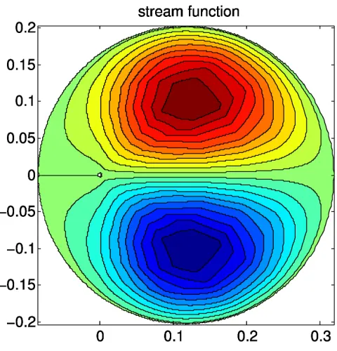
Two main observations were drawn from the numerical experiments of Gremaud et al. First, when vertical axisymmetry is broken, secondary circulation takes place, i.e., vφ
be-comes non-zero and leads to two counter-rotating cells perpendicular to the tilt axis, as in Fig. 1. Second, the computed circulation currents were much larger for a Matsuoka-Nakai material than for a von Mises one.
The numerically predicted components of velocity vh φ and v
h
r depend upon the choice of
model parameters and constitutive relation. When using the Matsuoka-Nakai relation, vh φ
varies strongly as a function of wall friction, µw, ranging from the same order as the radial
flow to three or more orders of magnitude smaller. Similar behavior is seen when the von Mises granular criterion is used, but the effect is smaller by orders of magnitude [16].
FIG. 1: Numerical simulations of tilted hoppers predict the rise of two secondary circulation cells,
rotating in opposite directions. The strength and shape of the cells depend on the angle of tilt,
angle of internal friction, and coefficient of wall friction. The azimuthal angleφis taken to be zero
on the line of symmetry between the two cells.
aboveµw = tan(θs) = 0.5, where the angle of friction of the simulated material wasθs= 30o
[14].
III. METHODOLOGY
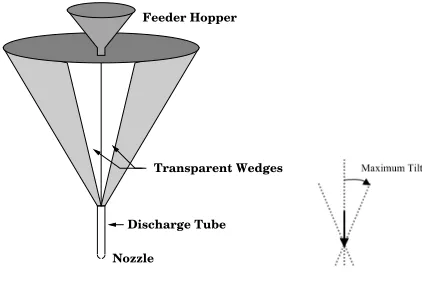
Our experimental test hopper is an approximately-conical, regular polyhedron composed of fourteen brass wedges (µw = 0.34 when bare) and two clear Plexiglas wedges. The hopper,
depicted in Fig. 2, is ∼45 cm wide at the top and the walls are angled at θw = 24o. Flow
Nozzle
Transparent Wedges Feeder Hopper
Discharge Tube
FIG. 2: Schematic of hopper in which we observe flowing sand. To perturb the flow we tilt the
hopper up to 23 degrees.
In these experiments we use Ottawa sand (ASTM C-190). The sand (coefficient of friction µsand= 0.42 and diameter 420≤d≤595µm) is mixed with a small quantity of tracer sand
that has been dyed dark red with instrument ink and repeatedly baked dry.
The entire hopper can be physically tilted. A digital (CCD) camera, bolted to the side of the hopper, tilts with the hopper and can be aligned with the Plexiglas “windows” in one of two configurations so that images showing the passage of sand may be recorded with a computer. The hopper is tilted so that the windows are on the axis of the tilt, where vφ is
predicted to be maximal. A plumb line is hung within the hopper and imaged to determine the direction of gravity in the frame of the camera for each tilt.
Since the conical hopper is made of flat wedges each wedge is oriented differently to form the cone. To account for the tilt of the camera relative to the orientation of the window wedges we mount the camera two different ways. In the first, we align the camera so that the tilts of the two windows are equal but opposite in orientation relative to the camera. In this arrangement, any geometric effect caused by the tilt of one window should be reversed in the other window.
We use the second camera arrangement when we line the walls of the hopper with ma-terials with different coefficients of friction. To minimize the impact of the viewing window when lining the hopper we cut a hole no bigger than the size of the field of view of the camera into the liner. In this case we align the camera flush with just one window of the hopper.
The coefficient of friction, µw, of a particular liner material is determined by using a
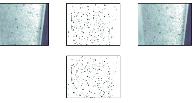
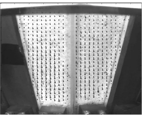
FIG. 3: Velocities are determined from identifying tracer particles and regressing over twenty-one
consecutive frames to assign a velocity to the eleventh frame. Shown here are the actual frames
(left) and thresholded tracer bitmaps (right) for a given frame (top) and the twentieth frame
later (bottom), corresponding to 40 s of experimental observation. The dark dots indicate centers
assigned to large tracer particles.
sand. We capture the motion of the tray using a high-speed digital camera and analyze the images to determine the acceleration of the tray. For each run there is a period where the forces on the sled are roughly constant and we perform a linear fit to the velocity in this region to determine acceleration. By varying the load applied to the tray as well as the weight acting through the pulley we can account for systematic frictional forces and deduce the sliding coefficient of friction for sand on the liner material.
Data sets for determining the velocity field typically consist of 1000 frames taken once every two seconds — covering roughly thirty-three minutes of flow. For a given combination of tilt and wall material, from two to six data sets are used to determine each plotted point for v.
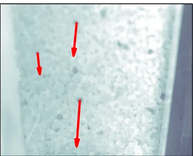
FIG. 4: The velocities assigned to the eleventh frame in the sequence depicted in Fig. 3 indicate
that in that frame only three tracer particles had sufficiently-long unambiguous tracks to be used.
Typically a dozen or more grains are tracked in a frame.
Since the grains are slightly irregular, the cluster identifying a given tracer grain changes as the particle rotates along the window surface. Typical tracer particles are roughly 20×20 pixels in size, though smaller dark or bright spots are tracked and used if possible. Each cluster is assigned a “center of mass” determined from the spatial distribution of its pixels, and then is identified with the nearest center of mass in the previous frame to construct a track of particle position in consecutive frames. If the nearest center of mass is outside a tunable maximum radius, the identification is rejected and a new particle track begins. Once a track is twenty-one frames long, a velocity is calculated using a least-squares fit and the interpolated velocity is assigned to the location of the tracer in the eleventh frame, as in Fig. 4, where out of the dozens of possible tracers only three are being used. If the velocity is zero, indicating an edge of the window is being tracked, it is ignored. Particle tracks begin and end as tracer particles move into and out of the field of view of the camera due to the overall flow and motion towards and away from the window — the mean track length is roughly 26 frames. In this manner we generate a time-integrated velocity field by binning velocities into regions by tracer location over the length of the run.
Once a velocity field is generated for a particular combination of tilt angle and wall friction, as in Fig. 5, we can calculate the ratio vφ/vr. If we have recorded using two,
FIG. 5: The time-averaged velocity field is generated by spatially binning the velocities for every
frame.
both components of velocity horizontally (fixed r) across the velocity field to the distance from the middle of the image to compensate for the slight tilt of the windows away from the camera. We interpolate using this fit to find the velocity components nearest the middle of the field of view of the camera from both windows, corresponding to φ =π/2 (φ = 0 is in the plane of the tilt). If we are using a single window, we perform a quadratic fit across the velocity field to account for φ variation (a higher order effect in the two-window case). We again interpolate the velocity components at φ=π/2.
We find both the azimuthal and radial components of the velocity to vary radially as 1/r2
, in agreement with mass conservation and the Jenike solutions. Given that both components vary as 1/r2
, the ratio of the two velocity components, vφ/vr, should be independent of r.
Linear fits to 1/r2
of the two velocity components are made and for each radial bin of the vector field the ratio of the vφ-fit to the vr-fit is calculated and the mean is recorded as the
observed ratio. Error bars are established using the standard deviation of these ratios.
IV. RESULTS
-0.2 -0.1 0 0.1 0.2 0.3
Tilt Angle
ε
(Radians)
-0.1 0 0.1 0.2
v
φ
/v
r
Left Window Right Window
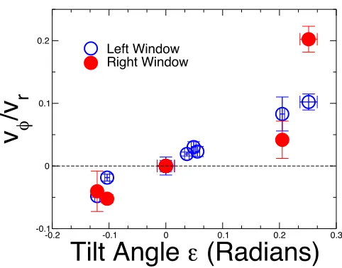
FIG. 6: The ratio of azimuthal to radial velocity for the right- (•) and left-hand (◦) windows for
a bare (µw = 0.34) hopper.
secondary-circulation. With careful alignment and balancing of our untilted experimental hopper we were able to reduce, but not completely eliminate, this apparent non-radial flow even for the untitled case. In order to compensate for the observed small non-radial component of the flow, we rotate the experimental images to a frame in which the untilted hopper flow is perfectly radial.
As the measurements from our test hopper shown in Fig. 6 indicate, in a bare brass hopper (µ= 0.34) secondary circulation does in fact follow linearly with tilt angle for small perturbations (% < 0.15). At larger angles, the dependence appears to depart from linear, which might be expected, since higher-order terms should eventually become important. Note that the ratio of azimuthal to radial velocity, vh
φ/vrh, follows systematically for tilts in
both directions, indicating that our observations are not an artifact. Numerically it is possible to predictvh
φ/vrh as a function ofµsand, θwall andµwall, although
-0.2 -0.1 0 0.1 0.2 0.3 0.4
Tilt Angle
ε
(Radians)
-0.2 -0.1 0 0.1 0.2
v
φ
/v
r
µ = 0.05 (Teflon)
µ = 0.26 (UHMWPE)
µ = 0.75 (Emery Paper)
Linear Fit to Bare Hopper Data (µ = 0.34)
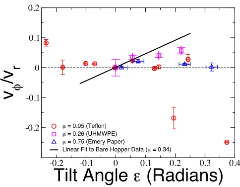
FIG. 7: Comparison of the ratio of azimuthal to radial velocity for Teflon (µw = 0.05 — (),
UHMWPE (µw= 0.26 —!) and Emery paper (µw = 0.75 —)) to a linear regression of the bare
(µw = 0.34) hopper observations (solid line).
As the tilt increases however, a strong azimuthal component is observed in the opposite direction of the flow in the bare hopper. The tilt angle for the onset of flow showed some variation, possibly indicating a bistable state, hysteretic effects or some other influence beyond the controls of the experiment.
As wall-friction is increased beyondµcritical, soil mechanics models of granular flow predict
a transition from mass-flow — where all the material in the hopper is moving — to funnel flow where there are non-moving, stagnant regions at the wall. However, when we line the hopper with Emery paper, which has a higher coefficient of friction µ= 0.75 than the interparticle frictionµcrit= tanθsand we continue to observe some radial flow at the window,
although there is no azimuthal component within measurement error.
Although extreme values of wall friction induce large changes in flow, we find that the flow is relatively robust to small variations in wall friction. Changing the wall friction slightly from the bare hopper (from µw = 0.34 to 0.26), by lining with low-friction Ultra-High
-0.2 -0.1 0 0.1 0.2 0.3
Tilt Angle
ε
(Radians)
-0.2 -0.1 0 0.1 0.2
v
azim
/v
r
von Mises Matsuoka-Nakai
FIG. 8: Ratio of azimuthal to radial velocity for a bare hopper as a function of hopper tilt angle"
as imaged through the right (•) and left (◦) windows of the test hopper, rotated to the frame where
the untilted flow is entirely radial. Lines indicate numerical predictions for von Mises (dotted) and
Matsuoka-Nakai (dashed) plasticity models.
0 0.1 0.2
Tilt
ε
(Radians)
-5x10⁻⁴
0
5x10⁻⁴
v
φ/v
r0 0.1 0.2 0.3 0.4
Tilt
ε
(Radians)
-0.3 -0.2 -0.1 0
v
φ/v
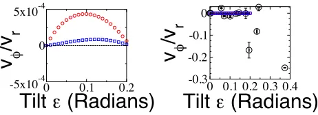
rFIG. 9: When wall friction is extremely low, µw = 0.05, the numerically-predicted ratio of
az-imuthal to radial velocity as a function of hopper tilt angle (left) is four orders of magnitude
smaller than the experimentally observed ratio at large tilt angles (right).
V. COMPARISON WITH SOIL MECHANICS PREDICTIONS
The dashed and dotted lines in Figure 8 show azimuthal to radial velocities ratios as calculated for varying tilts in a bare hopper using a spectral method [16]. We find that the values predicted using the Matsuoka-Nakai constitutive relation match our observations reasonably well for small angles, |%| < 0.1, while the granular von Mises relation predicts much too little circulation. This suggests that the Matsuoka-Nakai criterion may more accurately describe the yielding of dense granular flows in the regime we are studying.
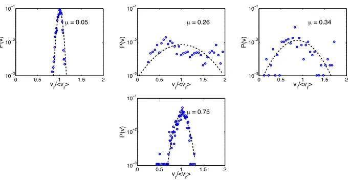
0 0.5 1 1.5 2 10−3
10−2
10−1
vr/<vr>
P(v)
µ = 0.05
0 0.5 1 1.5 2
10−3
10−2
10−1
vr/<vr>
P(v)
µ = 0.26
0 0.5 1 1.5 2
10−3
10−2
10−1
vr/<vr>
P(v)
µ = 0.34
0 0.5 1 1.5 2
10−3
10−2
10−1
vr/<vr>
P(v)
µ = 0.75
FIG. 10: The width of the probability distributions of radial velocity varies non-monotonically with
wall friction, with the extremes having much narrower distributions than more moderate friction
values. The distributions are roughly fit by Gaussians (dashed lines), with moderate values of
friction having positive skewness and extreme values having negative skewness.
when the hopper wall friction is lowered (e.g. Figure 7, teflon lining). The ratio vφ/vr is
numerically predicted to be very small for both the Matsuoka-Nakai and von Mises yield criteria, in agreement with what we observe for |%| < 0.2 but beneath the threshold to distinguish between them experimentally.
VI. VELOCITY FLUCTUATIONS
Although the numerical approach here describes the mean flow, we know that stress in hoppers is subject to large fluctuations about the mean [12]. Since Levy’s flow rule assumes that the velocity in our hopper is directly related to the stress, it is interesting to examine any fluctuations in our velocity distributions [17].
Previous work by Zhu and Yu using numerical Discrete Element Methods has studied the probability distribution of velocities in a flat-bottomed cylindrical hopper as wall friction was varied from µ = 0.1 to 0.5 [19]. Although their cylindrical system had notable differences from ours, including the presence of stagnant regions and plug flow, separate distributions for the radial component of flow were calculated, allowing rough comparison. In the DEM simulations it was found that the fluctuations decrease as wall friction is reduced.
−02 −1 0 1 2 0.02 0.04 0.06 0.08 0.1
v/<vr>
P(v)
a
−02 −1 0 1 2 0.02
0.04 0.06 0.08 0.1
vφ/vr
P(v
φ
/vr
)
b
−02 −1 0 1 2 0.02
0.04 0.06 0.08 0.1
v/<vr>
P(v)
c
−02 −1 0 1 2 0.02
0.04 0.06 0.08 0.1
vφ/vr
P(v
φ
/vr
)
d
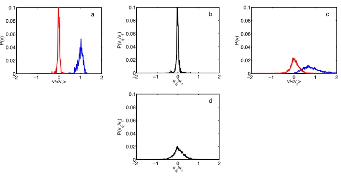
FIG. 11: Probability distributions of a) the azimuthal (left) and radial (right) components of the
velocity for flow in an untilted hopper,b) vφ
vr for an untilted hopper,c)the components in a hopper at tilt"= 0.14 andd) vφ
vr for"= 0.14. These results are for an Emery paper-lined hopper, although they are representative of other wall frictions.
the four wall frictions we examined. We generate our velocity histograms by scaling several sets of data by the mean radial velocity for that set. Since the mean velocity varied for some experiments, for each value of wall friction we use the largest data set with consistent radial velocities to generate our histograms. Within one data set, the velocity fluctuates sharply with time due to both our tracking technique which can produce frames in which no velocities are assigned and the large variability inherent to dense granular flows [20, 21]. The power spectrum for the time series does not indicate periodicity.
as the ratio of those two components for untilted and highly tilted cases. For both tilted and untilted hoppers the means are similar, but the distribution grows much wider with tilt angle. Interestingly, although the distributions are wider for the highly tilted hopper, the distribution of vφ/vr is of roughly the same width as that of vφ, indicating that the
fluctuations of the two components are correlated. This is associated with the fact that individual grains follow roughly fixed trajectories even if they are different from the mean flow. These persistent trajectories may indicate long-term correlation of particle contacts that might be expected for clusters of of grains moving together, such as the “granular eddies” of Erta¸s and Halsey [23].
VII. CONCLUSION
We have observed that real three-dimensional flows of granular matter are more complex than the idealized case of perfectly radial Jenike-like flow. In response to small perturbations (in the form of tilts), non-radial velocities arise leading to potentially large shifts in behavior. For small tilts we have found that the magnitude of circulation numerically predicted using the Matsuoka-Nakai constitutive relation is closer to observations than numeric predictions made with the more traditional, generalized von Mises condition. At larger tilts we observe that the non-radial flow becomes even more pronounced, exceeding numerical predictions for all constitutive relations.
We have examined the influence of wall friction and discovered that extreme values, low or high, act to suppress secondary circulation. In the case of large perturbations and low friction, we see an abrupt and unpredicted onset of secondary circulation in the opposite direction of the moderate friction case.
Acknowledgements
JFW and RPB acknowledge funding from National Science Foundation grants DMR-0137119, DMR0555431, and DMS-0204677 and NASA grant NNC04GB08G. PAG acknowl-edges funding from NSF Grants DMS-0244488 and DMS-0410561.
[1] R. Nedderman, Statics and Kinematics of Granular Materials (Cambridge University Press, 1992).
[2] H. Matsuoka and T. Nakai, Soils and Foundations 25, 123 (1985).
[3] H. Matsuoka, T. Hoshikawa, and K. Ueno, in Powders and Grains, edited by J. Biarez and R. Gourv´es (1989), pp. 339–346.
[4] D. G. Schaeffer, International Journal for Numerical and Analytical Methods in Geomechanics
14, 253 (1990).
[5] A. W. Jenike, Tech. Rep. 108, University of Utah (1961).
[6] J. Choi, A. Kudrolli, R. Rosales, and M. Bazant, Physical Review Letters92, 174301 (2004).
[7] S. Horl¨uck and P. Dimon, Physical Review E63, 031301 (2001).
[8] A. Medina, J. A. C´ordova, E. Luna, and C. Trevi˜no, Physics Letters A 250, 111 (1998).
[9] C. S. Chou, J. Y. Hsu, and Y. D. Lau, Physica A308, 46 (2002).
[10] J. R. Ducker, M. E. Ducker, and R. M. Nedderman, Powder Technology 42, 3 (1985).
[11] S. B. M. Moreea and R. M. Nedderman, Chemical Engineering Science51, 3931 (1996).
[12] G. W. Baxter, R. Leone, and R. P. Behringer, Europhysics Letters21, 569 (1993).
[13] G. H. Ristow, Ph.D. thesis, Philipps University-Marburg (1998).
[14] P. A. Gremaud, J. V. Matthews, and D. G. Schaeffer, SIAM Journal of Applied Mathematics
64, 583 (2003).
[15] P. A. Gremaud, J. V. Matthews, and M. O’Malley, Journal of Computational Physics 200,
639 (2004).
[16] P. A. Gremaud, J. V. Matthews, and D. G. Schaeffer, Journal of Computational Physics219,
443 (2006).
[17] A. W. Jenike, Powder Technology 50, 229 (1987).
[19] H. P. Zhu and A. B. Yu, Journal of Physics D 37, 1497 (2004).
[20] N. Menon and D. J. Durian, Science 275, 1920 (1997).
[21] E. Gardel, E. Keene, S. Dragulin, N. Easwar, and N. Menon, cond-mat/0601022 (2006).
[22] S. Moka and P. R. Nott, Physical Review Letters 95, 068003 (2005).