Original Research Open Access
Model choices to obtain adjusted risk difference estimates
from a binomial regression model with convergence
problems: An assessment of methods of adjusted risk
difference estimation
Mavuto Mukaka1,2,3,4*, Sarah A. White2, Victor Mwapasa2, Linda Kalilani-Phiri2, Dianne J Terlouw1,3 and E. Brian Faragher3
1Malawi-Liverpool-Wellcome Trust Clinical Research Programme, College of Medicine, University of Malawi, Malawi. 2Department of Public Health, College of Medicine, University of Malawi, Malawi.
3Liverpool School of Tropical Medicine, Pembroke Place, Liverpool, UK.
4Mahidol-Oxford Tropical Medicine Research Unit, Mahidol University, Ratchathewi District, Bangkok, Thailand. *Correspondence: [email protected]
Abstract
Background: Risk Difference (RD) is becoming the measure of choice for estimating effect size in antimalarial drug efficacy trials. Calculating RD using binomial regression is prone to model non-convergence. Cheung’s modified ordinary least squares (OLS) method is a proven technique for handling non-convergence when estimating RD. Other promising methods include the Poison, Additive Binomial Regression and binary regression models fitted using the statistical package R. (Deddens’) Copy method that was primarily developed to overcome non-convergence of log-binomial regression models when estimating risk ratios is another potential method. Simulations were conducted to compare the performance of the Copy method against four alternatives (Cheung’s modified OLS method, the Additive Binomial Regression Model fitted with the blm algorithm, the binary regression model fitted with the glm2 algorithm, and the Poisson model with identity link and robust standard errors fitted with the glm algorithm) for obtaining RD estimates when a binomial model fails to converge.
Methods: We computed estimates of efficiency and bias with treatment arm efficacies of (a) 60% vs. 85%, (b) 95% vs. 90%, (iii) 95% vs. 98% using simulation studies. A total of 5,000 datasets were simulated under each of these three scenarios.
Results: The modified OLS method and the binary regression model fitted using the glm2 algorithm in R provided unbiased, efficient estimates of RD across all assessed scenarios. In contrast, the Copy method yielded biased estimates of RD even when 100% convergence was achieved. The Poisson and Additive Binomial Regression models had 100% and almost 100% convergence rates respectively, but both produced very slightly biased RD estimates.
Conclusion: The Copy method is not suitable for estimating RD when binomial regression model fitting fails to converge. Cheung’s modified OLS or the binary regression model fitted using the glm2 algorithm in R should be the method of choice to overcome non-convergence with binomial models for calculating adjusted RD estimates.
Keywords: Copy method, risk difference, binary outcome, binomial model, Cheung’s modified least squares estimation, simulation, bias
© 2016 Mukaka et al; licensee Herbert Publications Ltd. This is an Open Access article distributed under the terms of Creative Commons Attribution License (http://creativecommons.org/licenses/by/3.0). This permits unrestricted use, distribution, and reproduction in any medium, provided the original work is properly cited.
Introduction
The most common measures for comparing binary outcomes between two groups include: a risk ratio (RR), an Odds Ratio (OR) and a risk difference (RD).
CrossMark
The risk ratio (RR) is an appropriate summary statistic in cohort studies where study participants are selected on the basis of their exposure to the risk factor of interest. However, the risk difference provides an appealing, informative alternative ef-fect estimate and increasingly is being used in randomized controlled trials.
One pitfall of the RR is the possibility of incorrect inter-pretation. For example, the risk ratio for the outcome being a success is not the inverse of the risk ratio for the (same) outcome being a failure [1], although the two ratios are complementary and should ideally lead to the same conclu-sion. Of particular concern is that, when risk ratios are used in Randomized Controlled Equivalence Trials, evidence of equivalence in the failure rates of two treatments does not necessarily imply evidence of equivalence in the success rates of the same two treatments [2]. The same may be true for non-inferiority studies also. A risk difference, on the other hand, has the same value irrespective of whether success or failure is modelled, so is a preferable headline summary statistic if only on the grounds of ease, and consistency, of interpretation.
Furthermore, when the failure levels are very low in both treatment arms, modeling treatment failure may result in a large risk ratio that represents only a small failure risk differ-ence. For example, consider a situation where the treatment failure rates for treatment A and B are 1% and 4% respectively. The treatment failure risk ratio (B to A) is 4; in simple terms, individuals receiving treatment B are 4 times more likely to experience a treatment failure than those receiving treat-ment A. Even if the sample size is sufficient for this RR to be statistically significantly different from the null hypothesis value of 1, it only reflects a RD of 3%. Of course, if “failure” is death, this may be a fair and sensible indication of the rela-tive efficacy of the treatments – but in many contexts, for example if failure is incomplete resolution of the symptoms associated with the common cold within a pre-specified time period, the real clinical significance of this difference may be considered to be small or even negligible. In this latter scenario, a RD is probably a more informative measure of relative treatment efficacy.
Two final considerations that may be important when se-lecting the most appropriate summary statistic for indicating the relative sizes of treatment effects: the confidence intervals (CIs) for RRs are not symmetric about the estimate (except on the log scale), which may serve to ‘exaggerate’ true relative effect; while many researchers continue to favor reporting odds ratios (ORs) in prevalence studies on the basis that many previous studies of a similar nature to their own have reported this statistic, it is a simple matter of fact that the interpretation of an OR is difficult for many researchers [3].
In summary, risk difference (RD) is often the effect measure of choice, particularly for malaria treatment efficacy studies, the focus of this paper. The RD has the considerable advantage of being much easier to interpret than the most commonly
used alternatives, RR and OR, and produces the same value irrespective of whether success or failure is measured so is flexible to use in practice. Unfortunately, however, the serious practical problems that can be experienced when calculat-ing RD values can exceed these advantages and either RR or (most usually) OR values are calculated.
Technically, the most straightforward way of calculating risk differences is by using standard binomial regression methods, but these are prone to convergence failure – and these model non-convergence problems increase as one or both efficacy levels approach a boundary value (i.e. as these approach either 0% or 100%), for the mathematical reasons described below.
Estimation of probabilities in a risk difference model using binomial regression
Consider the following generalized linear model (GLM):
g(u)=α+β1X1+β2X2 +………..+βkXk (1)
where g(u) is a link function identifying a function of the mean that is a linear function of the covariates;
X1, X2, ………., Xkform a set of k explanatory variables such as age, sex, location, etc.
Using an identity link with a response on a continuous scale in the above GLM model would yield a multiple linear regression model.
When the outcome is binary, u (often alternatively repre-sented as π) in this model is the probability of observing a specific category of the binary outcome. The GLM with binary outcome and identity link reduces to:
g(u) = π=α+β1X1+β2X2 + ……….. +βkXk (2)
Because the expression α+β1X1+β2X2 + ……….. +βkXk is unbounded, the estimate of π is a linear function of the explanatory vari-ables and can thus yield estimates of outcome probabilities that are outside the valid range of 0 to 1.
Let us now reconsider equation (2).If X1 is a binary expo-sure (0 or 1) denoting the treatment / intervention to which an individual is randomized in a clinical trial, the estimate of the adjusted risk difference (RD) becomes:
RD =
π
ˆ
1-π
ˆ
0 (3)Substituting from equation (1) gives:
RD=[(a b1*1+b2X2+ ……+bkXk)–(a+b1*0+b2X2+ ……..+bkXk)] (4a)
where a and bi are estimates of α and βi respectively. When, as occurs in most conventional clinical trials, there are only two treatments this reduces to:
For a binary outcome and binary exposure, equation (5a) reduces to
RD =
π
ˆ
1−
π
ˆ
0 (5b)which is exactly the same as the RD estimated by a binomial regression [2].
Cheung shows that using the Huber-White robust estimate of variance for the OLS RD gives the same variance as that provided by the maximum likelihood binomial regression. The Huber-White estimate of variance in matrix form is given as:
Where X is the design matrix with xi as the ith row of the matrix;
is the residual
y
i−
x
ib
; is the vector of OLS estimates.The OLS estimate of the risk difference is just b1. In contrast to the estimation of probabilities, this has less stringent boundary constraints suggesting that, if the interest is in estimating the risk difference rather than the individual risks (probabilities) themselves, estimates of the risk difference based on the above linear model would be valid.
Cheung demonstrated both algebraically and using simula-tions that Ordinary Least Squares estimation methods with Huber White standard errors are valid for the estimation of risk differences. This method also avoids the non-convergence problems that can be experienced when using a binomial regression model with an identity link function [2]. Cheung’s modified least squares method is a simple method with appealing properties that can be applied in many standard software packages.
Deddens and Petersen [4] proposed the Copy method to
address the problem of non-convergence when estimating risk ratios with the log-binomial model using Maximum Likeli-hood Estimation (MLE). Non-convergence usually occurs when the effect estimates are near the boundary of the parameter space (when either or both of the risk estimates is close to 0% or 100%, the risk ratio itself is either close to zero or ap-proaching infinity). As its name suggests, in this approach multiple copies of the dataset are added to the original set. For a risk ratio, the Copy method involves calculating MLEs using a log-binomial model on an expanded version of the data set that contains K-1 copies of the original dataset plus one copy of the original dataset in which the values of the binary outcome variable are reversed (the 1’s (successes) are all changed to 0’s (fails) and the 0’s (fails) are all changed to
1’s (successes)). For a log-binomial model, if the total number of dataset copies, K, is finite, the estimate is an MLE for the “copied” dataset [5]. When the binomial regression model is applied to this modified data set, the model converges and approximate maximum likelihood estimates of the risk ratio are obtained [4-6].
Petersen and Deddens [5,6] recommend that K should be at least 100 (in their paper they used a value of K=1,000). The standard error estimates for the MLEs obtained with the Copy method are based on K copies so have to be multiplied by √(K) to convert them to estimates for the original (single) dataset. Mathematically, expanding the original data set in the manner required for the copy method is simply equiva-lent to creating a new data set consisting of one copy of the original data set, having a weight of K-1, and one copy of the original data set with the outcome values reversed, having a weight of one. Lumley [7] showed that use of the weights (K-1)/K and 1/K for the original outcome and the reversed outcome datasets respectively eliminates the need to adjust the standard error [7].
A number of methods have been suggested for estimating (adjusted) risk differences. Early methods were based either on simple formulas derived from odds ratios (Greenland and Holland [8]) or on generalized linear models (Wacholder [9]). Later methods include a modified Poisson regression model fitted using the software package SAS [10]; this involves some very simple and straightforward coding but as SAS is expensive it is often not accessible by many researchers, and there are well documented situations in which this model fails to converge [2,11].
Another approach proposed for calculating model-adjusted risk difference estimates uses mean marginal predictions from a logistic regression model ([11]). This model can be fitted with the SUDAAN software package which is capable of handling complex data; algorithms for fitting this model are also available for software packages such as SPSS and Stata but again the cost of these may be prohibitive for some researchers. Almost certainly, this model can be fitted using the free software package R;, however, although R is perfectly capable of handling complex statistical analyses, we note that Stata/SPSS users frequently fail to migrate to R even after several attempts due to the steep learning curve involved. In addition, Williamson, Eliasziw and Fick [12] experienced convergence problems with this and less standard models in all of the software packages they used, including both R and Stata. Even the powerful SAS software package sometimes failed to converge for the log-binomial model [12,13], and convergence failed with Stata due to the iterations going to a wrong place and then being unable to return to the parameter space.
It is acknowledged that several methods have been pro-posed to tackle the problem of non-convergence. As most of these focus on risk ratio estimation with only a few attempt-ing to tackle this problem in the context of risk difference
1 1 1
1 OLS 2
2 1
1
(
)(
)
RD
(
)
n n n
i i i i
i i i
n
n i i
i i
y x
y
x
b
x
x
n
= = =
= =
−
=
=
−
∑
∑
∑
∑
∑
(5a)
(6)
-1 2 -1
1
ˆ
Var( ) (X'X) (
b
=
∑
ni=e x x
i i' )(X'X)
ii
estimation, however, we agree with Williamson [12] that, despite the increasing volume of research being published attempting to deal with non-convergence in log-binomial models, this problem still exists, especially when estimating risk differences. There have been recent extensive develop-ments in software packages such as SAS, Stata and SUDAAN attempting to resolve problems of non-convergence. The most attractive and promising of these appear to be in R, for example fitting Additive Binomial Regression Models with the blm algorithm, fitting the binary regression model using the glm2 package, and fitting the Poisson model with identity link and robust standard errors through the glm algorithm.
The Binomial linear model (BLM) is defined as follows: Let Y be a binary random variable. Under the binomial linear model (BLM), the probability of an outcome is a linear function of a covariates x, is:
P(Y=1| x)=xTβ
where Y=1 if the outcome is observed and 0 otherwise [14]. Each of the estimated coefficients of β is the adjusted risk difference as-sociated with a unit increase in the corresponding covariate [14]. Although Cheung’s modified OLS and BLM appeared to be possible solutions to the problem of model non-convergence, we could find no documented evidence in the literature on whether or not the copy method can be applied to overcome non-convergence when fitting a binomial regression model using the identity link function to obtain risk differences. Thus, to address this, we used simulation methods to assess the performance of the copy method when applied to risk difference modeling in situations where the original binomial model fails to converge, comparing its performance to four alternatives: the established Cheung’s modified OLS method, the Additive Binomial Regression Model output with the blm package, the binary regression model fitted via glm2 pack-age in R, and the Poisson model with identity link and robust standard errors fitted via glm in R.
Methods
In order to simulate covariate data that reflected a real life situation, parameter values were derived from a malaria drug efficacy study conducted in Malawi between 2003 and 2006 [15]. The covariates of interest were hemoglobin (Hb), age and weight (wt) because these are likely to be associated with both treatment and outcome, consequently there may be need to adjust for them when estimating treatment effect. That is, they are potential confounders. Outcome data were simulated for three different scenarios using Bernoulli distributions: (i) with an efficacy level of 0.85 (85%) for group A and 0.60 (60%) for group B, a true absolute efficacy difference of 0.25 (25%); (ii) an efficacy level of 0.90 (90%) for group A and 0.95 (95%) for group B; and (iii) an efficacy level of 0.98 (98%) for group A and 0.95 (95%) for group B. The aim of considering these dif-ferent efficacy levels was to allow for generalizability of the
findings across a range of outcome scenarios.
Parameter values for simulation of covariates and the assessment criteria
The simulations were performed using the Stata 13 software. For each scenario 5,000 simulated datasets were used. The covariates in each model were hemoglobin (Hb), age and weight. Treatment group was included as a factor.
The matrices of parameters for simulating the baseline covariates were as follows:
where: X is a vector of the three covariates (measured on a logarithmic scale for age and wt but using the original scale units for hemoglobin (Hb));
μ is a vector of the mean values for log(age), Hb; log(weight) respectively.
The outcome was simulated as a binary variable with the desired success rates in each group. Models involving treat-ment group as a factor and age, Hb and weight as covariates were fitted under the following strategies:
1. Binomial regression on the original dataset.
2. The copy method with K values ranging between 10 and 100,000.
3. Cheung’s modified OLS method.
4. The binary regression model fitted via glm2 package in R. 5. The Poisson model with identity link and robust standard errors fitted via glm package in R software.
6. The Additive Binomial Regression Model fitted via the blm package in R software.
The following statistics were obtained from each of these analyses: the percentage of simulated datasets for which the model fitting converged, the degree of bias in the MLEs of the true efficacy difference and the average (mean) 95% lower and upper limits of the confidence intervals statistical coverage.
Results
Simulation results
Standard binomial regression model
In all three of the simulated scenarios, convergence problems were encountered when the binomial regression model was fitted (Table 1). The problem worsened as efficacy rates approached a boundary value. Even when neither rate was near a boundary, approximately 5% of the models failed to converge. When both efficacy rates were at least 95%, however, model fitting failed to converge for over 60% of the simulated
datasets. When convergence did occur, the estimates were biased for each of the scenarios investigated. Coverage was unacceptably low, being just under 90% for the scenario involving 60% and 85%efficacy rates and below 40% for the scenario where both efficacy levels were close to 100%.
Cheung’s modified OLS method and binary regression model fitted via glm2 in R
The Cheung’s modified OLS approach and the binary regres-sion model fitted using the glm2 algorithm in R performed consistently well across the range of scenarios considered in terms of convergence rates and bias (Tables 2 and3). There was 100% convergence and the mean bias was zero for all three assessed scenarios. The coverage was high being around 95% for all assessed scenarios for the OLS approach while the binary regression model fitted using glm2 was conservatively
too high being 100% for all the scenarios being investigated.
Poisson model with identity link and robust standard errors fitted via glm in R
The Poisson model with identity link and robust standard er-rors fitted using the glm algorithm in R also achieved 100% convergence but experience some, arguably negligible, bias in the estimated RD values (Table 4). The coverage was too high being 100% for all the scenarios that we considered.
Additive Binomial Regression Model fitted via blm in R
The Additive Binomial Regression Model fitted using the blm algorithm in R software experienced some non-convergence but in only a few simulated sets. The convergence rates were above 98%. Some (negligible) bias was observed (Table 5). The Statistical coverage was very variable and to high for some
Efficacy rates
(%) TrueRD Converged N (%) Estimated RD (SE) 95% CI*LL UL Coverage (%) Bias
85 vs 60 0.250 4755 (95.1) 0.240 (0.060) 0.122 0.358 0.896 -0.010
90 vs 95 0.050 3550 (71.0) 0.037 (0.036) -0.034 0.108 0.162 -0.013
98 vs 95 0.030 1987 (39.7) 0.036 (0.025) -0.013 0.085 0.360 +0.006
Table 1. Percentage convergence, efficiency, coverage and bias for the binomial model for each scenario.
Table 2. Percentage convergence, efficiency, coverage and bias for Cheung’s OLS method of RD estimation for each scenario.
Table 3. Percentage convergence, efficiency, coverage and bias for binary regression model using glm2 algorithm in R.
Table 4. Percentage convergence, efficiency, coverage and bias for Poisson model with identity link and robust standard errors using glm algorithm in R.
amean SE over 5000 simulations, *mean lower and upper CIs over 5000 datasets
amean SE over 5000 simulations, *mean lower and upper CIs over 5000 datasets
amean SE over 5000 simulations, *mean lower and upper CIs over 5000 datasets
amean SE over 5000 simulations, *mean lower and upper CIs over 5000 datasets
Efficacy rates
(%) True RD Converged N (%) RD (SE)
a 95% CI* Coverage (%) Bias
LL UL
85 vs 60 0.250 5000 (100) 0.250 (0.061) 0.130 0.369 0.950 0.000
90 vs 95 0.050 5000 (100) 0.050 (0.037) -0.022 0.122 0.945 0.000
98 vs 95 0.030 5000 (100) 0.030 (0.026) -0.021 0.079 0.950 0.000
Efficacy rates
(%) True RD Converged N (%) RD (SE)
a 95% CI* Coverage Bias
LL UL
85 vs 60 0.250 5000 (100) 0.250 (0.061) 0.130 0.370 100 0.000
90 vs 95 0.050 5000 (100) 0.050 (0.037) -0.023 0.123 100 0.000
98 vs 95 0.030 5000 (100) 0.030 (0.026) -0.021 0.081 100 0.000
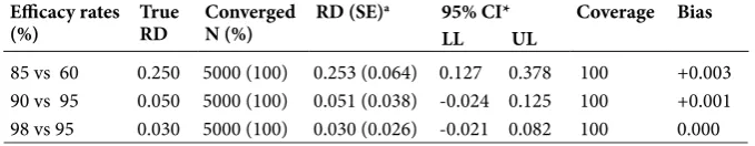
85 vs 60 0.250 5000 (100) 0.253 (0.064) 0.127 0.378 100 +0.003
90 vs 95 0.050 5000 (100) 0.051 (0.038) -0.024 0.125 100 +0.001
98 vs 95 0.030 5000 (100) 0.030 (0.026) -0.021 0.082 100 0.000
Efficacy rates
(%) True RD Converged N (%) RD (SE)
a 95% CI* Coverage Bias
scenarios. The coverage was 91.8% for the 98% vs 95% efficacy rates; 98.5% for the 95% vs 90% efficacy scenarios and 100% for the 85% vs 60% efficacy scenarios.
Simulation results: Deddens’ Copy method
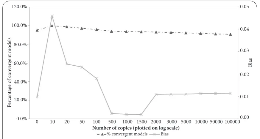
For each simulated scenario, the percentage of non-convergent models was least when the number of copies (K) used was 10. When 20 or more copies were used, the percentage of non-convergent models increased (Figures 1-3) and continued to do so consistently as K was increased. However, for all three scenarios, the non-convergence rates were better than the rate obtained using no copies for up to at least 100 copies, although beyond 5,000 copies the non-convergence rates were worse for all the scenarios. In addition, some datasets that converged when analyzed conventionally failed to con-verge when the copy method was adopted.
Bias was observed irrespective of the number of copies used. With just 10 copies, risk difference was underestimated in all three scenarios. Tables of the parameter estimates are presented in detail in Supplementary Tables S1-S3.
Discussion
The Copy method did not provide a remedy to the
non-conver-gence problem when modeling risk differences. These findings agree with those reported by Petersen and Deddens [5] and also by Chen, Shi and Qian [16] in a discussion of their finding that non-convergence occasionally occurs for log-binomial models even if the COPY method is applied. So, while the Copy method has been found to be effective in solving non-convergence problems when using log-binomial models to estimate risk ratios [4-6], our findings demonstrate clearly that the method is not appropriate for modeling risk differences. In all of the simulation scenarios we considered, 100% con-vergence was often achieved when around 10 copies were used but this was found to be the number of copies at which the estimates for the risk difference were most biased. Increasing the number of copies beyond 10 simply increased the likeli-hood of non-convergence. The most likely explanation for this is that, although close to 100% convergence can be achieved with K=10, the effect of the reversed copy is not diluted suf-ficiently to provide unbiased estimates of risk differences. Perhaps surprisingly at first glance, convergence failure rates became more common when the number of copies was increased beyond 5000, but this is due to the fact that increasing K yields an outcome distribution similar to the original in which the binomial model failed, thus resulting Efficacy rates
(%) True RD Converged N (%) RD (SE)
a 95% CI* Coverage(%) Bias
LL UL
85 vs 60 0.250 4999 (99.9) 0.250 (0.067) 0.120 0.379 100.0 0.000
90 vs 95 0.050 4985 (99.7) 0.047 (0.026) -0.003 0.097 98.5 -0.003
98 vs 95 0.030 4945 (98.9) 0.026 (0.013) -0.000 0.051 91.8 -0.004
Table 5. Percentage convergence, efficiency, coverage and bias for Additive Binomial Regression Models using blm algorithm in R.
amean SE over 5000 simulations, *mean lower and upper CIs over 5000 datasets
Figure 1. Percentage Convergence and (absolute) Bias for selected Numbers of Copies (85% vs. 60%). 0 10 20 50 100 500 1000 1500 2000 3000 5000 10000 50000 1000000.00
0.01 0.02 0.03 0.04 0.05 120.0%
100.0%
0.0%
Per
cen
ta
ge o
f co
nv
er
gen
t m
ode
ls
80.0%
60.0%
40.0%
20.0%
Bi
as
in the model failing again. Hence the finding that datasets that did not converge with the original binomial model also tended to be more likely to fail to converge with the Copy method, particularly when large numbers of copies were made. Some of the datasets that were convergent with the origi-nal binomial regression model become non-convergent with the Copy method. A possible reason for this is that the Copy method creates very large datasets. In general, very large and very small datasets are both susceptible to non-convergence problems [13]. In addition, bias patterns were found to be
very irregular with increasing number of copies, probably because fitted models that converge do not do so at random; those models that fail to converge when just a few copies are used will also fail to converge when more copies are added. This was not explored in any more depth in this paper as our primary focus was merely on whether the non-convergence problem would be solved or not.
The Cheung’s modified OLS method and the binary re-gression model fitted using the glm2 algorithm in R appear to be the optimum approaches for estimating adjusted risk Figure 2. Percentage Convergence and (absolute) Bias for Increasing Numbers of Copies (95% vs. 90%).
Figure 3. Percentage convergence and (absolute) bias for increasing numbers of copies (98% vs. 95%). 0 10 20 50 100 500 1000 1500 2000 3000 5000 10000 50000100000
Number of copies (plotted on log scale)
0 10 20 50 100 500 1000 1500 2000 3000 5000 10000 50000 100000
Number of copies (plotted on log scale)
120.0%
100.0%
0.0%
Per
cen
ta
ge o
f co
nv
er
gen
t m
ode
ls
80.0%
60.0%
40.0%
20.0% 120.0%
100.0%
0.0%
Per
cen
ta
ge o
f co
nv
er
gen
t m
ode
ls
80.0%
60.0%
40.0%
20.0%
0.00 0.01 0.02 0.03 0.04 0.05 0.00 0.01 0.02 0.03 0.04 0.05
differences. Our findings confirm that both of these methods not only converge but also provide unbiased estimates of risk differences when standard methods of binomial regression fail to converge. Both methods remains robust even when several covariates are included in the regression model, mak-ing them useful for controllmak-ing for potential confounders and also for identifying independent predictors of outcome when modeling risk differences. In addition, the methods yield unbiased estimates of risk differences with robust standard errors, thus offering clear statistical advantages over the use of the binomial regression method when the binomial model fails to converge. Efficient standard errors for the modified OLS are obtained via Huber-White standard errors. However the glm2 binary regression model suffers from too high (conservative) statistical coverage that remained at 100% for all scenarios. This coverage property puts Cheung’s OLS at a statistical property advantage over the glm2 model.
The Poisson model with identity link and robust standard errors fitted using the glm algorithm in R also emerged in our simulations as a promising method for estimating risk differ-ences. Model convergence is assured using this approach; while some bias can be expected with this method, it is likely to be very minimal. Minimal bias risk also occurred when the Additive Binomial Regression Model was fitted with the blm algorithm in R, but disappointingly a small chance of model non-convergence was also identified.
Conclusion
The standard binomial model with an identity link function is the method of first choice for estimating risk/efficacy dif-ferences, provided the model converges. When a model fails to converge, this problem can be addressed most efficiently using either Cheung’s modified OLS approach or by fitting a binary regression model with the glm2 package in R; both of these methods converge and provide efficient unbiased esti-mates of adjusted risk differences. The Cheung’s OLS method offers a statistical coverage property over the glm2 approach. The Poisson model with identity link and robust standard errors fitted using the glm algorithm in R and the Additive Binomial Regression Model fitted using the blm algorithm in R are possible alternatives as they have 100% and almost 100% convergence rates respectively, but both produce very slightly biased risk difference estimates. In addition the Poisson model has too high coverage while the blm approach produces variable statistical coverage depending on efficacy scenarios. The Copy method is not a suitable approach for estimating ad-justed risk differences and is now effectively rendered obsolete in the presence of methods such as Cheung’s modified OLS and the binary regression model fitted using the glm2 package in R.
Additional files
Competing interests
The authors declare that they have no competing interests. Authors’ contributions
Acknowledgement
This work was supported by the European and Developing Countries Clinical Trials Partnership (EDCTP) grant number IP.2007.31060.03; and the Johns Hopkins University Center for AIDS Research (Grant Number1P30AI094189) from the National Institute of Allergy And Infectious Diseases. Publication history
EIC: Jimmy Efird, East Carolina University, USA. Received: 12-Feb-2016 Final Revised: 14-Mar-2016 Accepted: 25-Mar-2016 Published: 05-Apr-2016
Supplementary Table S1 Supplementary Table S2 Supplementary Table S3
Authors’ contributions MM SAW VM LK DJT BF Research concept and design ✓ ✓ ✓ ✓ ✓ ✓ Collection and/or assembly of data ✓ ✓ -- -- -- ✓ Data analysis and interpretation ✓ ✓ -- -- -- ✓ Writing the article ✓ ✓ ✓ ✓ ✓ ✓ Critical revision of the article ✓ ✓ ✓ ✓ ✓ ✓ Final approval of article ✓ ✓ ✓ ✓ ✓ ✓ Statistical analysis ✓ -- -- -- --
--References
1. Blizzard L and Hosmer DW. Parameter estimation and goodness-of-fit in
log binomial regression. Biom J. 2006; 48:5-22. | Article | PubMed
2. Cheung YB. A modified least-squares regression approach to the
estimation of risk difference. Am J Epidemiol. 2007; 166:1337-44. |
Article | PubMed
3. Greenland S. Interpretation and choice of effect measures in
epidemiologic analyses. Am J Epidemiol. 1987; 125:761-8. | Article |
PubMed
4. Deddens J and Petersen MR. Estimation of prevalence ratios when PROC
GENMOD does not converge. In: Proceedings of the28th Annual SAS
Users Group International Conference. Cary, NC: SAS Institute Inc. 2003; 270-28 . | Pdf
5. Petersen MR and Deddens JA. A revised SAS macro for maximum
likelihood estimation of prevalence ratios using the COPY method. Occup Environ Med. 2009; 66:639. | Article | PubMed
6. Deddens JA and Petersen MR. Approaches for estimating prevalence
ratios. Occup Environ Med. 2008; 65:481, 501-6. | Article | PubMed
7. Lumley T, Kronmal R and Ma S. Relative risk regression in medical
research: models, contrasts, estimators, and algorithms. UW
Biostatistics Working Paper Series. 2006; 293.
8. Greenland S and Holland P. Estimating standardized risk differences
from odds ratios. Biometrics. 1991; 47:319-22. | Article | PubMed
9. Wacholder S. Binomial regression in GLIM: estimating risk ratios and risk differences. Am J Epidemiol. 1986; 123:174-84. | Article | PubMed
10. Spiegelman D and Hertzmark E. Easy SAS calculations for risk or
prevalence ratios and differences. Am J Epidemiol. 2005; 162:199-200. |
Article | PubMed
11. Bieler GS, Brown GG, Williams RL and Brogan DJ. Estimating
model-adjusted risks, risk differences, and risk ratios from complex survey data. Am J Epidemiol. 2010; 171:618-23. | Article | PubMed
12. Williamson T, Eliasziw M and Fick GH. Log-binomial models: exploring failed convergence. Emerg Themes Epidemiol. 2013; 10:14. | Article |
PubMed Abstract | PubMed FullText
13. SAS/STAT(R) 9.2 User’s Guide SEe. SAS Technical Support. 2009. |
14. Kovalchik S and Varadhan R. Fitting Additive Binomial Regression Models with the R Package blm. Journal of Statistical Software. 2013; 54. 15. Bell DJ, Nyirongo SK, Mukaka M, Zijlstra EE, Plowe CV, Molyneux ME,
Ward SA and Winstanley PA. Sulfadoxine-pyrimethamine-based
combinations for malaria: a randomised blinded trial to compare efficacy, safety and selection of resistance in Malawi. PLoS One. 2008;
3:e1578. | Article | PubMed Abstract | PubMed FullText
16. Chen W, Shi J, Qian L and Azen SP. Comparison of robustness to outliers
between robust poisson models and log-binomial models when estimating relative risks for common binary outcomes: a simulation study. BMC Med Res Methodol. 2014; 14:82. | Article | PubMed Abstract
| PubMed FullText
Citation:
Mukaka M, White SA, Mwapasa V, Kalilani-Phiri L, Terlouw DJ and Faragher EB. Model choices to obtain adjusted risk difference estimates from a binomial regression model with convergence problems: An assessment of methods of adjusted risk difference estimation. J Med Stat Inform. 2016; 4:5.