Accuracy of MFCC-Based Speaker Recognition
in Series 60 Device
Juhani Saastamoinen
Department of Computer Science, University of Joensuu, P.O. Box 111, 80101 Joensuu, Finland Email:[email protected]
Evgeny Karpov
Department of Computer Science, University of Joensuu, P.O. Box 111, 80101 Joensuu, Finland Email:[email protected]
Ville Hautam ¨aki
Department of Computer Science, University of Joensuu, P.O. Box 111, 80101 Joensuu, Finland Email:[email protected]
Pasi Fr ¨anti
Department of Computer Science, University of Joensuu, P.O. Box 111, 80101 Joensuu, Finland Email:[email protected]
Received 1 October 2004; Revised 14 June 2005; Recommended for Publication by Markus Rupp
A fixed point implementation of speaker recognition based on MFCC signal processing is considered. We analyze the numerical error of the MFCC and its effect on the recognition accuracy. Techniques to reduce the information loss in a converted fixed point implementation are introduced. We increase the signal processing accuracy by adjusting the ratio of presentation accuracy of the operators and the signal. The signal processing error is found out to be more important to the speaker recognition accuracy than the error in the classification algorithm. The results are verified by applying the alternative technique to speech data. We also discuss the specific programming requirements set up by the Symbian and Series 60.
Keywords and phrases:speaker identification, fixed point arithmetic, round-offerror, MFCC, FFT, Symbian.
1. INTRODUCTION
The speech research and application development deal with three main problems: speech synthesis, speech recognition, and speaker recognition. We are working in a speech tech-nology project, where one of the main goals is to integrate automatic speaker recognition technique into Series 60 mo-bile phones.
In speaker recognition, we have a recorded speech sam-ple and we try to determine to whom the voice belongs. This study involvesclosed-set speaker identification, where an un-known sample is compared to previously trained voice mod-els in a speaker database.
The speaker identification is a speech classification prob-lem. Based on the training material, we create speaker-specific voice models, which divide the feature space into dis-tinct classes. Unknown speech is transformed to a sequence of features, which are scored against voice models. That speaker is identified and his model has the best overall match
with the input features. There are many ways to choose the used features and how they are used. Our research team has studied, for example, how the feature design [1], or the con-current use of multiple features [2], affects the recognition accuracy.
Our speaker identification method is a generic automatic learning classification with mel-frequency cepstral coefficient (MFCC) features. The classification algorithm that we use in this study is a common unsupervised vector quantizer. We have ported the identification system to a Series 60 Symbian mobile phone. In this study, we introduce the Series 60 plat-form and the ported system. In particular, we focus on the numerical analysis of the signal processing algorithms which had to be converted to fixed point arithmetic.
Decision Speaker recognition classify input speech based on existing profiles
Read and use all profiles during recognition
Speaker profile database Add/remove speaker profiles during training Speech
audio Signal processing and
feature extraction Feature vectors
Speaker modeling create speaker
profile
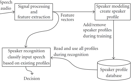
Figure1: Closed-set speaker identification system.
our proposed system. For example, with 100 TIMIT speak-ers, the recognition rates for different implementations are 100% (floating point), 9.7% (straightforward fixed point), and 95.8% (proposed system).
2. SPEAKER IDENTIFICATION SYSTEM
We consider a speaker identification system with separate modules for speech signal processing, training and classifi-cation, and speaker database (Figure 1). The system oper-ates in training mode or recognition mode. The two different chains of arrows starting from the signal processing module describe the data flow (Figure 1).
The system input in training mode is a collection of speech samples fromNdifferent speakers. A signal process-ing model is applied to produce a set of feature vectors for each speaker separately. Then a mathematical model is fitted to the feature vector set. We use thevector quantization(VQ) model to represent the statistical distribution of the features of each speaker. Each feature vector set is replaced by a code-book, which is a smaller set ofcode vectors with fixed size. Codebooks are stored in the speaker database to represent the speakers. A common goal of the codebook design is to min-imize the quantization distortion of the training data, that is, we look for code vectors which minimize the distortion, when training vectors are replaced by their nearest neigh-bors in the codebook. We use thegeneralized Lloyd algorithm (GLA) [3] to generate the codebook.
In therecognition mode, the input speech sample is pro-cessed by the same signal processing methods as in the train-ing. The features are quantized using each codebook in the database. The speaker whose codebook gives the least dis-tortion is identified. If needed, the system lists the smallest distortions and corresponding speakers.
The signal processing module computes MFCC features (Figure 2). They are commonly used in speech recognition [4]. The speech is divided into overlapping frames. Within a frame, the signal is preemphasized and multiplied by a win-dowing function before computing the Fourier spectrum. A mel-filter bank is applied to the magnitude spectrum, and logarithm of the filter bank output is finally cosine
Feature vector
DCT Log Filter
bank Absolute
DFT Time
windowing Preemphasis
Digital speech signal frame
Figure2: MFCC signal processing steps.
transformed. The first coefficient of the cosine transform is omitted as it depends on the signal energy. We want to dis-card absolute energy information which depends, for exam-ple, on the distance to the microphone, or on the voicing de-gree. If we kept the first coefficient, then the vectors with high overall intensity, for example vowels, would dominate the distance computations. Only part of the cosine-transform output coefficients are used as the feature vector.
3. SYMBIAN ENVIRONMENT
The small size of mobile phones is demanding for manufac-turers. A hardware design must be cheap to manufacture, fit in small space, and have low power consumption.
The company Advanced RISC Machines (ARM) has de-veloped the most commonly used mobile phone processors. They are fully 32-bit RISC processors with a 4 GB address range. A three-stage pipeline is used, which allows execution of one instruction per every cycle [5].
One drawback of the ARM processors is that they have no floating point support because of its complexity and hard power consumption.
3.1. Symbian OS and Series 60
In order to reduce phone development costs, the leading manufacturers started developing an industry standard op-erating system for advanced, data-enabled mobile phones [6]. The company Symbian was formed in 1998 by the leaders of the mobile industry: Nokia, Ericsson, Panasonic, Motorola, Psion, Siemens, and Sony Ericsson. They devel-oped theSymbian OS operating system [7], which evolved from the EPOC operating system developed by Psion. It has a modular microkernel-based architecture [6], whose core consists ofbase(microkernel and device drivers),middleware (system servers), andcommunications(telephony, messaging, etc.) [6].
The Symbian OS can be combined with different user interface (UI) platforms. A UI platform is a set of pro-grammable UI controls, which all have similar style. There are three UI platforms known to the authors: UIQ (oped by Sony Ericsson), Series 60, and Series 80 (both devel-oped by Nokia).
3.2. Programming for Symbian OS
Programs for Symbian OS can be written in Java and C++. The Java API and execution speed are limited, so C++ is used for computationally intensive programs. A lot of APIs are available for the C++ programmer, and there is also a lim-ited ANSI C standard library [6,7].
The main difference to conventional PC programming in Symbian OS is that the program must always be ready for ex-ceptional situations. Device can easily use all available mem-ory or program can be interrupted by incoming phone call, which has higher priority. Programs must also be as small and efficient as possible to not overwhelm the limited hard-ware resources. Robustness is also important, because mobile phones are supposed to work without restart for months or even more [7].
The used algorithms must be selected carefully, numer-ically stable low-time complexity methods are preferred. There is no hardware floating point support. There exists a software implementation of double-precision floating point arithmetic but it should be used rarely because of its com-plexity and higher power consumption. Also there is a 64-bit integer type available for the programmer, but it is a software implementation where the data is stored in a pair of 32-bit integers. The ported algorithms must be efficient, therefore we use fixed point arithmetic and only native data types, that is, integers whose basic operations are directly supported by the processor.
3.3. C++ restrictions
The Symbian OS restricts the use of C++ features. There is no standard exception handling. Symbian designers im-plemented their own mechanism for it, mainly because the GCC compiler used in target builds did not support it at the time [7]. Consequently, a C++ class constructor cannot cre-ate other objects. It might cause an exception, and Symbian has no way to handle exceptions thrown from a constructor. Therefore, atwo-phase constructionmust be used, where ob-ject creation and initialization are separated [7]. As another consequence, the memory stack is not unrolled after an ex-ception, so the programmer must use acleanup stack frame-work, which unrolls the stack automatically after an excep-tion [7]. That is why all objects allocated from the heap must be derived from a common base class (CBase), added to the stack immediately after allocation, and removed only just be-fore deletion [7]. Here, conventional C++ compiler duties have become manual programming tasks.
Efficiency requirements dictate another important aspect of Symbian programming. Applications or DLLs can be ex-ecuted from the ROM without copying them first to the RAM. It creates another programming limitation: an appli-cation stored in a DLL has no modifiable segment and cannot
use static data [7]. However, Symbian provides athread-local
storagemechanism for static data [7]. Basically, any
applica-tion interacting with the user is stored in a DLL and loaded by the framework, when a user selects to execute the particu-lar program [7].
We implemented most of the computational algorithms in the ANSI C language and used the POSIX standard where applicable. The reasons were good portability, an existing prototype written in C, and the ANSI/POSIX support of the system. The Symbian OS has a standard C library, so pro-grams are easy to port to it. The main limitation is that static data, that is, global variables cannot be used. Also file handling is restricted: fopen and other file-processing func-tions may not work as expected in multithreaded programs. The developers are encouraged to use the providedfile server mechanisms instead.
4. NUMERICAL ANALYSIS OF MFCC AND VQ IN FIXED POINT ARITHMETIC
During the recognition, the speaker information carried by the signal propagates through the signal processing (Figure 2) and classification to a speaker identity decision. The mappings involved in the MFCC process are smooth and numerically stable. In fact, the MFCC steps are one-to-one mappings, except those where the mapping is to a lower-dimensional vector space, for example, computing magni-tudes of the elements of the complex Fourier spectrum.
The MFCC algorithm consists of evaluations of different vector mappings f between vector spaces, denote such eval-uation by f(x). A computer implementation evaluates val-ues f(x), wherexis an approximation ofx represented in a finite-accuracy number system, and the computer imple-mentation ftries to capture the behavior of f. When im-plementing f, we aim at minimizing therelative errorof the values f(x),
= f(x) −f(x)
f(x) , (1)
instead of theirabsolute errorf(x)−f(x). The motivation for using relative error is that all elements of all vectors, dur-ing all MFCC stages, may carry information that is crucial to the final identification decision. The importance of each el-ement to the final speaker discrimination is independent of the numerical scale of the data in the subspace correspond-ing to the element. The inputxis usually the output of the previous step.
We consider a system capable of fixed point arithmetic with signed integers stored in at most 32 bits. The input con-sists of sampled signal amplitudes represented as signed 16-bit integers. In many parts, we use different integer value in-terpretation, a scaling integerI >1 represents 1 in the normal algorithm. Often we must also divide input, output, or inter-mediate result to ensure that it fits in a 32-bit integer. We now analyze the system.
4.1. Preemphasis
Many speech processing systems apply apreemphasisfilter to the signal before further processing. The difference formula yt = xt −αxt−1is applied to the signal xt, our choice is a commonα=0.97. The filter produces output signalytwhere higher frequencies are emphasized and lowest frequencies are damped.
4.2. Signal windowing
Numerically speaking, there is nothing special in the signal windowing. A signal frame is pointwise multiplied with a
window function. The motivation is to avoid artifacts in the
Fourier spectrum that are likely to appear because of the signal periodicity assumption in the Fourier analysis the-ory. Therefore, the window function has usually a taper-like shape, such that the multiplied signal amplitude is near-original in the middle of the frame but gradually forced to zero near the endpoints. Getting the multiplied signal grad-ually to zero requires using enough bits to represent the win-dow function values. For example, in the extreme case of us-ing only one bit, the transition from original signal to a ze-roed multiplied signal is sudden, not gradual. We use 15 bits in the experiments.
4.3. Fourier spectrum
The frequency spectrum is computed as theN-pointdiscrete
Fourier transform(DFT)F :CN →CN,
F(x)= N−1
k=0
e−2πiωk/Nxk, ω=0,. . .,N−1. (2)
As a linear map,F has a corresponding matrixF ∈CN×N, andF(x) can be computed as the matrix-vector productFx using O(N2) operations. Theradix-2 fast Fourier transform
(FFT) [8] utilizes the structure of F and computes Fx in O(NlogN) operations forN=2m,m >0. The FFT executes the computations in log2Nlayers ofN/2butterflies,
fl+1
k =fkl+Wklfkl+T,
fkl++1T =fkl−Wklfkl+T.
(3)
Superscripts denote the layer and the constants Wkl ∈ C are called twiddle factors. The first layer input is the signal
f0
k =xk,k =0,. . .,N−1. The offset constantTvaries be-tween layers, the value depends on whether the FFT element reordering [8] is done for input or output.
4.3.1. Existing fixed point implementations
The FFT efficiency is based on the layer structure. However, fixed point implementations introduce significant error. The round-offerrors accumulate in the repeatedly applied but-terfly layers.
Our reference FFT is C code generated by thefftgen soft-ware [9]. he generated code computes the squared FFT mag-nitude spectrum (Section 4.4) of a signal in fixed point arith-metic. The butterfly layers and the element reordering are all merged in few subroutines, with all loops unrolled. It uses 16-bit integer representation for the input signal, intermedi-ate results between layers, and the automatically computed power spectrum output. Multiplication results in (3) are 32-bit integers, but stored in 16-32-bit integers after shifting 16 32-bits to the right in order to keep the next layer input in proper range. Overflowing 16-bit result of addition and subtraction in (3) is avoided by shifting their inputs 1 bit to the right. The truncations increase error and introduce information loss.
We employed the generated FFT code in the fixed point MFCC implementation and compared it to the floating point counterpart. The MFCC outputs computed from identical inputs with the two implementations did not correlate much. It might originate from the accumulation of errors in the MFCC process. However, detailed analysis showed that the greatest error source is FFT (DFT inFigure 2). We also ver-ified that the error does not originate from the final trunca-tion of the power spectrum elements to 16 bits, but from the FFT algorithm itself. In order to verify it, we tuned the gen-erated code to output the complex FFT spectrum instead of the power spectrum.
Many techniques have been developed for decreasing the error in fixed point implementations. A comprehensive anal-ysis of various possibilities was presented by Tran-Thong and Liu in [10]. There are also many improvements tailored for specific microprocessors and applications. For example, Sa-yar and Kabal consider an implementation for a TMS320 dig-ital signal processor [11].
4.3.2. Proposed FFT
Our approach is more general than the implementations listed above. We consider any processor capable of integer arithmetic with signed 32-bit integers. We use an existing radix-2 complex FFT implementation [12] as the starting point. First, we change the data types, additions, and mul-tiplications similar to thefftgen-generated code.
Consider the DFT in the operator form f =Fx, and our implementation f = Fx. The approximation error f − f consists of the input error x−x and the implementation error. SinceFandFare linear, the implementation error is F−F. This is not exactly true, as we have a limited-accuracy numeric implementation, which is only linear up to the nu-meric accuracy.
Now repeat the same analysis but consider a linear but-terfly layer in the FFT algorithmg=Gy, and its implementa-tiong=Gy. The inputsycarry information about accurate valuesy, that is, information about the signalx. In the butter-fly (3), each multiplication of the layer input elementfkl∈C with the operator constantWkl ∈Cexpands to two additions and four multiplications of real values. If we use more than 16 bits for the real values that correspond to fl
k, then we must use less bits for the real values that correspond to the oper-ator constantWkl, in order to represent the real values that correspond to the multiplication result with 32 bits.
We allow increase in the relative error of the layer op-erator G −G/G, meanwhile the relative input error y−y/yis decreased so that more information about yfits intoy, and more is preserved in the multiplication re-sult. Consequently, more information aboutypropagates to the next layer input gin all layers, therefore less informa-tion is lost in the whole FFT. We increase the FFT opera-tor errorF−F/Flittle but preserve more information aboutx. Consequently, the relative errorFx−Fx/Fx decreases. This is the main idea and it can also be applied to other algorithms implemented in fixed point arithmetic. Here the norm of a linear operator Ais defined asA = maxx=1Ax/x, and the differenceA−Bof the
opera-torsAandBis defined by (A−B)x=Ax−Bx, for allx.
4.3.3. Bit allocation
The twiddle factors of anN-point DFT are constructed from the values±sinπk/Nand±cosπk/N,k=0,. . .,N/2−1. Be-fore deciding how the bits are allocated for the signal and the operator, we look at the relative trigonometric value round-offerrors for different FFT sizesNand bit allocationsB >0. For eachB, we look for a scaling integercwhich gives small value of the maximum error
E(c,N)= max k=0,...,N/2−1
sk−sk
sk , (4)
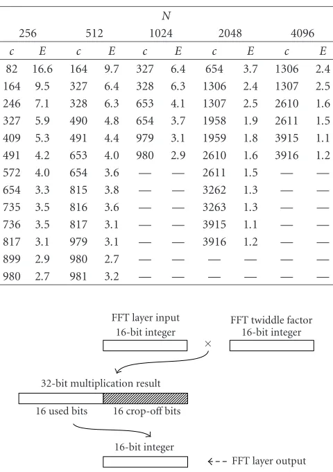
wheresk=csinπk/Nandskdenotesskrounded to the near-est integer. It is enough to consider only the positive sines, since the cosine values are in the same set. ForN=256, 512, 1024, 2048, and 4096, there are several peaks downwards in the graph ofE(c,N) as a function ofc. They are good choices ofc, even if they do not minimizeE(c,N).Table 1shows the pairs of good values ofcandE(c,N) for differentN. The bit allocationBis defined as the number of bits needed to store c.
We decided to limit the FFT size toN ≤ 1024 and not minimizeE(c,N) for eachNseparately. For allN=256, 512, and 1024, the valuec=980 is the best choice withB=10.
Table1: Pairs of valuescandE(c,N) for different FFT sizesN, the pairs are selected whereEis small; the values of the functionEhave been multiplied by 103.
N
256 512 1024 2048 4096
c E c E c E c E c E
82 16.6 164 9.7 327 6.4 654 3.7 1306 2.4 164 9.5 327 6.4 328 6.3 1306 2.4 1307 2.5 246 7.1 328 6.3 653 4.1 1307 2.5 2610 1.6 327 5.9 490 4.8 654 3.7 1958 1.9 2611 1.5 409 5.3 491 4.4 979 3.1 1959 1.8 3915 1.1 491 4.2 653 4.0 980 2.9 2610 1.6 3916 1.2 572 4.0 654 3.6 — — 2611 1.5 — — 654 3.3 815 3.8 — — 3262 1.3 — — 735 3.5 816 3.6 — — 3263 1.3 — — 736 3.5 817 3.1 — — 3915 1.1 — — 817 3.1 979 3.1 — — 3916 1.2 — —
899 2.9 980 2.7 — — — — — —
980 2.7 981 3.2 — — — — — —
FFT twiddle factor 16-bit integer ×
FFT layer input 16-bit integer
32-bit multiplication result 16 used bits 16 crop-offbits
16-bit integer
FFT layer output
Figure3: Multiplication of a 16-bit integer, followed by a bit shift in a layer of thefftgenFFT.
That leaves 22 bits for the signal information. Thus, we re-place the signal/operator bit allocation 16/16 with 22/10. The choice with onecfor allNandB =10 is good enough for us, as we mostly use N = 256. The diagrams in Figures 3-4 illustrate the bit allocation in integer multiplications and truncations in a layer of thefftgenFFT and the proposed FFT.
4.3.4. Evaluation of the accuracy
We compare the proposed fixed point solution to thefftgen generated FFT code. In our floating point MFCC implemen-tation, we compute FFT using theFastest Fourier Transform
in the West(FFTW) C library [13]. The FFTW relative error
is very small. We refer to FFTW output as the accurate so-lution when comparing the fixed point algorithms. We use a TIMIT speech segment as the input signal, resampled at 8 kHz (Figure 5).
FFT twiddle factor 16-bit integer, 10 bits used ×
FFT layer input 32-bit integer, 22 bits used
32-bit multiplication result 22 used bits 10 crop-offbits
32-bit integer, 22 bits used
FFT layer output
Figure4: Multiplication of a 22-bit integer, followed by a bit shift in a layer of the proposed FFT.
0 2000 4000 6000
−7000 0 7000
PCM
sample
value
Sample index
Figure5: A speech sample from the TIMIT corpus.
Comparison of the FFT magnitude scatter plots in Fig-ures 6-7shows that in fixed point arithmetic, we may de-crease the error by using the integer scale more efficiently. The proposed FFT is accurate without scaling also. Also note that the proposed FFT has an increased range of accurate val-ues, that is, the distance along the diagonal from the right-most observation to the place where the observations start to deviate from the diagonal is much longer for the proposed FFT than thefftgenFFT.
The statistical distribution of the relative error of the fixed point FFT elements is very skew, but the logarithmic error behaves nearly like a normal distribution. The his-tograms in Figures8-9illustrate the distribution of log10= log10(|fk−fk|/|fk|), which is the same as the signal-to-noise ratio in decibels divided by−10. Here fkand fkare elements of the correct FFT and the fixed point FFT, correspondingly. ThefftgenFFT error histogram is shown inFigure 8, whereas Figure 9shows the error of the proposed FFT. For statistical analysis, it makes sense to consider the logarithmic errors. Their interpretation is easier because of the original skew er-ror distribution.
Table 2summarizes the logarithmic error statistics. The numbers −0.775 and−2.118, for example, suggest that for the test signal, the proposed method has less than 1% error per element on average, whereas the same value is more than 10% for thefftgen. In terms of signal-to-noise ratio, the ad-vantage of our method is 13.43 dB for the original signal, and also a significant 10.32 dB for the more optimally scaled sig-nal. The statistics state clearly that the proposed FFT is a lot more accurate.
1 1000 1e + 006
FFTW output 0
1000 1e + 006
ff
tge
n
FFT
output
(a)
1 1000 1e + 006
FFTW output 0
1000 1e + 006
ff
tge
n
FFT
output
(b)
Figure6: Scatter plot offftgenFFT output against FFTW output for the TIMIT signalx(a) and 4x(b), scales are logarithmic.
Until now, we have only described the advantages of the proposed FFT but it also has little drawbacks. The scaling of the numbers between the FFT layers requires more opera-tions than thefftgenimplementation.
rep-1 1000 1e + 006 FFTW output
0 1000 1e + 006
P
roposed
FFT
output
(a)
1 1000 1e + 006
FFTW output 0
1000 1e + 006
P
roposed
FFT
output
(b)
Figure7: Scatter plot of proposed FFT output against FFTW out-put for the TIMIT signalx(a) and 4x(b), scales are logarithmic.
resented using integers. Therefore, before the addition and subtraction in a butterfly (3), we must scale up fl
k before adding it to the result of the complex multiplicationWklfkl.
In other parts of the MFCC algorithm, the more accurate 22-bit representation of the proposed FFT output could be utilized instead of scaling down to 16 bits. However, based on our error analysis and the statistic inTable 2, the 16-bit output offftgenFFT is really not accurate up to 16 bits, and neither is the proposed FFT. On average, there are 3–5 most significant bits correct in thefftgenFFT output and 7-8 most significant bits correct in the proposed FFT. Thus, there is no need to use more than 16 bits for the real part and 16 bits for the imaginary part of the FFT output elements.
−6 −4 −2 0 2
0 1000 2000
O
b
se
rv
ed
fr
eq
ue
ncy
Logarithm of the relative error (a)
−6 −4 −2 0 2
0 1000 2000
O
b
se
rv
ed
fr
eq
ue
ncy
Logarithm of the relative error (b)
Figure8: Histogram of logarithmic relative error values for theff t-genFFT with input signalsx(a) and 4x(b), the error increases to the right.
4.4. Magnitude spectrum
The Fourier spectrum is{fk ∈C; k =0,. . .,N/2−1}, the power spectrum is {|fk|2 ∈ R}, and the magnitude
spec-trum is{|fk| ∈R}. The squaring has no significant effect in the recognition rate for the floating point implementation. In fixed point arithmetic, the usage of the number range is not uniform for the power spectrum. The distribution of values |fk|2is dense for small|fk|and sparse for large|fk|. The
−6 −4 −2 0 2 0
1000 2000
O
b
se
rv
ed
fr
eq
ue
ncy
Logarithm of the relative error (a)
−6 −4 −2 0 2
0 1000 2000
O
b
se
rv
ed
fr
eq
ue
ncy
Logarithm of the relative error (b)
Figure9: Histogram of logarithmic relative error values for the pro-posed FFT with input signalsx(a) and 4x(b), the error increases to the right.
Without loss of generality, assume that |a| ≥ |b| and |a|>0 for fk=a+ ib. We may write
fk=
a2+b2= |a|
1 + b a
2
, (5)
where 1 + (b/a)2∈[1, 2] always. By introducing a parameter
t= |b/a| ∈[0, 1], we can approximate|fk|with
fk= |a|
1 +t2≈ |a|P
n(t), (6)
Table2: Average (AVG) and standard deviation (SD) of the base-10 logarithm of the relative error, and signal-to-noise ratio (SNR) in decibels for two FFT implementations, applied to the same signal on two different scales.
Used FFT Input AVG SD SNR (dB)
fftgen x −0.775 0.797 7.75
fftgen 4x −1.374 0.797 13.74
Proposed x −2.118 0.590 21.18
Proposed 4x −2.406 0.687 24.06
wherePn : [0, 1] → [1, √
2] is a polynomial of ordern≥1 with the boundary conditions
Pn(0)=1, Pn(1)= √
2. (7)
In order to satisfy boundary conditions, we actually find the orthogonal projection of√1 +t2−(1 + (√2−1)t) into the
function space spanned by the set of functionsS= {t−t2,t−
t3,t−t4,t−t5}, that is, fit a least-squares polynomial. Our
approximation is
1 +t2≈1 +√2−1t
−0.505404t−t2+ 0.017075t−t3
+ 0.116815t−t4−0.043182(t−t5, (8)
with the maximum relative error 1.30×10⁻⁵.
The motivation for our boundary conditions (7) is that a least-squares polynomial often has a relatively large maximal error in the endpoints of the approximation interval. Here the polynomial is used for evaluation of MFCCs, and accu-rate approximation is needed regardless oft, the ratio of real and imaginary parts of fk.
4.4.1. Complex magnitude with fixed point numbers
There probably are numerically better choices for the basis besidesS. However, it is straightforward to evaluatetp+1from
tpandtin our scaled integer arithmetic. Moreover, the basis Smeets the boundary conditions. Note also that 0≤t,tp,t− tp ≤ 1 fort ∈ [0, 1] so that all intermediate results in the polynomial evaluation are always within our number range.
In the fixed point implementation, we choose an integer scaling factor d ∈ [1, 215) to represent 1, because the
mul-tiplication results must always fit in 32 bits. The valuetand coefficients of 1,t,. . .,t−t5, are evaluated to rescaled
inte-gers before the polynomial evaluation. We chosed=20263 because it minimizes the average relative round-offerror in the scaled polynomial coefficients. The fixed point arithmetic square root approximation is
202631 +t2≈20263 + 8393t
−10241t−t2+ 346t−t3
+ 2367t−t4−875t−t5,
where the originalt ∈[0, 1] is multiplied withdand trun-cated to integer before the evaluation. During the evaluation, all multiplication inputs are within [0,d] and multiplication results are always divided withd. The maximum relative er-ror is 1.855×10⁻⁵fort=0.9427.
4.5. Filter bank
Applying a linear filter in the frequency domain is techni-cally similar to the signal windowing in the time domain, a spectrum is pointwise multiplied with a frequency response. Each filter output is a weighted sum of the magnitude spec-trum or power specspec-trum values. Applying alinear filter bank (FB) means applying several filters, and it is the same as com-puting a matrix-vector product where matrix rows consist of the filter frequency responses.
Numerically, the fixed point implementation is not com-plicated, we just need enough bits to represent the frequency response values. By our standard, we are using enough bits if a graphical visualization of the filter bank filters realizes our visual idea of the desired filter shape. We use 7 bits in the experiments, Technically, the purpose of filter bank is to measure energies in subbands of the frequency domain of the signal, with possible overlap between adjacent subbands. It is commonplace to define the filter bank so that
(i) for all input spectrum elements, the sum of weights over all filters is the same;
(ii) the width of the filters is defined by a monotonic
frequency-warping function[4], such that
(a) in the warped frequency domain, all filters have equal spacing, width, and overlap;
(b) in the warped frequency domain, all filters have the same shape, for example, triangular or bell.
The shape of filters is not important for speaker recognition but the choice of the frequency warping function has sig-nificant effect on the recognition accuracy [1]. Our choice is the commonly used, although not optimal mel-frequency warped FB with triangular filter shape.
One could argue that the FB smoothing effect compen-sates the numeric error of the FFT and magnitude computa-tions. However, discrimination information will be lost both in the numeric round-offand in the smoothing.
4.6. Logarithm
The nonnegative FB outputs are transformed into logarith-mic scale during the MFCC processing. Several methods for evaluation of log2have been introduced in [14] and there is a thorough error analysis in [15].
We use a modification of the method in [14], which uses a lookup table and linear interpolation. Consider an integer n >0 whose bit representation is
n=0 0 0 0 1bm. . . b1
m+1 bits
. (10)
The integer part of log2n is m. The decimal part is en-coded in the bitsbm,. . .,b1. We use the 8 most significant bits
bm,. . .,bm−7 as an index to a lookup table consisting of the
values log2(1+j/256),j=0,. . ., 256. The next 7 bits form the interpolation coefficients between two consecutive lookup table values. The maximum relative error 4.65×10⁻⁶occurs
forn = 272063, where the correct value is log2272063 = 18.053581 and our approximation is 18.053497.
4.7. Discrete cosine transformation
Discrete cosine transformation (DCT) is a linear invertible
mapping, which is most efficiently computed using the FFT and some additional processing. In our application, we trans-form 25–50-dimensional vectors to 10–15-dimensional vec-tors and use only part of the DCT output, so we compute it with the direct formula without FFT. We utilize the most common DCT form called DCT-II [16],
µj= NFB−1
k=0
lkcos π NFB k
+1 2
j
, (11)
where j = 0,. . .,NMFCC−1, andNMFCC is the number of
the MFCC coefficients needed. The inputlkconsists of the FB outputs or their logarithms,k=0,. . .,NFB−1. Usually,
µ0 is ignored as it only depends on the signal energy. The
DCT-II form is orthogonal ifµ0is multiplied by 1/
√ 2 and all coefficients are output [16]. DCT is applied to FB outputs in speech applications for many reasons. Here the rescaling and decorrelating of the FB outputs improves the clustering and the VQ classification.
We did not carefully analyze the DCT error in the fixed point implementation. The reason is that we found out that the FFT and the logarithm were the MFCC accuracy bottle-necks. We simply assign the scaling factor 32767 for cosine values and truncate 16 bits from the 32-bit input values. We might gain accuracy by similar analysis that we did with the FFT but not much. In contrast to the FFT, the direct DCT computation has only one layer.
4.8. Model creation and recognition
The GLA algorithm [3] constructs a codebook{ck}that aims at minimizing the MSE distortion
MSE(X,C)= N
j=1
min
1≤k≤K
xj−ck2
(12)
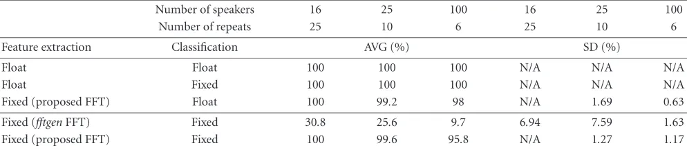
Table3: Recognition rate average and standard deviation for five different implementations of the MFCC-based speaker recognition system,
varying number of speakers taken from the TIMIT corpus and number of repeated cycles of training, and recognition.
Number of speakers 16 25 100 16 25 100
Number of repeats 25 10 6 25 10 6
Feature extraction Classification AVG (%) SD (%)
Float Float 100 100 100 N/A N/A N/A
Float Fixed 100 100 100 N/A N/A N/A
Fixed (proposed FFT) Float 100 99.2 98 N/A 1.69 0.63
Fixed (fftgenFFT) Fixed 30.8 25.6 9.7 6.94 7.59 1.63
Fixed (proposed FFT) Fixed 100 99.6 95.8 N/A 1.27 1.17
In speaker identification, the distortion (12) of input speech is computed for codebooks of all speakers stored in the speaker database. The result is a list of speakers and matching scores, sorted according to the score.
5. SPEAKER RECOGNITION EXPERIMENTS
In our training-recognition experiments, we use 8 kHz signal sampling rate,α=0.97 for the preemphasis, 30-millisecond frame length, 10-millisecond frame overlap, Hamming win-dow, FFT size 256, 30 filters in mel FB, and 12 coefficients from the DCT. The GLA speaker modeling uses 5 different random initial solutions picked from the training data. The codebook size is 64. We use 1-norm in (12) instead of the usual 2-norm. Everything else is kept as defined above. The motivation for using the 1-norm is the decreased computa-tional complexity. Before the experiments, we compared two systems where the only difference was the norm in (12) and there was no difference in recognition rates between 1-norm and 2-norm.
5.1. Simulations with PC
The TIMIT corpus has 630 speakers, 10 speech files per speaker. We divided them into independent training and test data consisting of 7 and 3 files, correspondingly. The results of the TIMIT experiments are listed inTable 3.
There are three columns of average recognition rates and three corresponding columns of standard deviations in Table 3. The statistics are computed for recognition rates in repeated cycles of training and recognition for subsets of 16, 25, and 100 speakers from the TIMIT corpus. The effect of the random initial solutions for the GLA, that are sampled from the training data, is taken into account in two ways. First, for each of the three TIMIT subsets, we use the same randomly picked GLA initial solutions in all experiments with the different computational techniques. On the other hand, repeating the same run with same technique but dif-ferent GLA initial solutions informs us about the effect of randomness in the recognition accuracy. The standard devi-ation of the recognition rate measures it. If the recognition rate was the same in all repeats, we inserted “not available” (N/A) for the standard deviation. The used number of re-peated training and recognition cycles was 25 repeats for the
16-speaker subset, 10 repeats for the 25-speaker subset, and 6 repeats for the 100-speaker subset.
For all used database sizes, the accurate floating point im-plementation of the MFCC-based speaker identification per-forms perfectly. The same is true even if we use the accurate features with a less accurate fixed point classification. If we use the fixed point features (proposed FFT) in combination with the floating point classification, the recognition rate de-creases slightly. Based on this, we conclude that the numer-ical accuracy of the signal processing is more important to the recognition accuracy than the numerical accuracy of the classification.
When we use the straightforward fixed point implemen-tation, less than 10 out of 100 speakers are identified cor-rectly. The reason is the FFT inaccuracy. When the fftgen FFT is replaced by the proposed FFT, the recognition rate in-creases near the 100% level again.
5.2. Mobile phone
We tested our implementation in a Nokia 3660 mobile phone for some time outside the laboratory conditions. The recog-nition accuracy was poor and we decided to investigate the effect of different signals. We created a 16-speaker GSM/PC corpus of dual recordings, which was later extended to con-sist of 25 speakers. The speech was recorded to two files si-multaneously with a Symbian phone via the Symbian API, and with a laptop that was equipped with a basic PC mi-crophone. The PC microphone was attached to the side of the phone with a rubber band. Each recorded file consists of nearly 1 minute of speech. All speakers spoke the same text.
For each speaker, the recording program was started manually in both devices, so the signal contained in the pairs of recorded sound files are little misaligned. The first 16 files were clear speech. The extended data set has many files with a mixture of speech and a lot of impulsive noise caused by scratching the microphones. However, we used all available data in the experiments.
Table 4: Recognition rate average and standard deviation for GSM/PC experiments with 25 speakers, 5 repeated cycles of train-ing, and recognition.
Audio Software AVG SD
PC Float 100.0 N/A
PC Fixed 100.0 N/A
Symbian Float 83.2 4.38
Symbian Fixed 76.0 2.83
time by using a multiresolution algorithm, so that we have file pairs where the only difference is the used microphone. There were 3 pairs in the extended data set where our auto-matic time-alignment method could not perfectly align the pair of signals. Those files were used as such regardless of a possible misalignment. After the MFCC computation, fea-tures resulting from all files were similarly split into separate training and test segments.
We repeated the training and recognition cycle 5 times for all combinations of GSM and PC data, and two im-plementations (the floating point implementation and the proposed algorithm). We eliminated the effect of the random GLA initial solutions by using the same initial solutions for both data sets and for the different implementations.Table 4 lists the results. If the recognition rate was the same in all repeats, we inserted “not available” (N/A) for standard devi-ation.
Based on the statistics inTable 4, we conclude that the Symbian sound recordings have a negative effect on the speaker recognition accuracy, when compared to PC micro-phone recordings of the same speech. Also we notice that the recognition rate depends on whether we use floating point arithmetic or fixed point arithmetic. However, the au-dio source is the most significant factor.
6. CONCLUSION
We ported an MFCC-based speaker identification method to Series 60 mobile phone. We encountered four problems: lim-ited memory, numeric accuracy, processing power, and Sym-bian programming constraints. A careful numerical analy-sis helped us to achieve good recognition accuracy in the fixed point implementation. The memory usage and compu-tational complexity of the speaker identification algorithms are low enough for interactive operation in today’s mo-bile phones. The Symbian programming constraints require some learning effort from a programmer familiar with more common platforms.
The numerical accuracy of the MFCC signal processing is important to the speaker recognition, especially the FFT accuracy. Recognition is accurate with floating point sig-nal processing, even if fixed point arithmetic is used for the classifier. If we combine fixed point signal processing (pro-posed FFT) and the accurate classification, the recognition rate slightly decreases. The signal processing accuracy is more important for correct recognition than the classifier accuracy.
The recognition results are poor when only fixed point arithmetic is used by the system and we are using thefftgen FFT. When the FFT is replaced by the proposed FFT, the re-sults are good again. The FFT seems to be the most critical part in the fixed point implementation.
Further improvement could be obtained by utilizing a better filter bank [1], and replacing DCT with a transforma-tion which is optimized for discriminatransforma-tion of speakers.
The FFT we implemented has a double loop. The inner-most loop table indexes are computed from the outerinner-most loop index. A better solution would integrate the proposed accuracy improvements in thefftgenmethod.
We also plan to include in our Symbian port the speed improvements that were introduced in [17].
The sound quality is currently the biggest problem. The audio system of the phone attenuates frequencies below 400 Hz and above 3400 Hz, because these are not needed in telephone networks. This has a negative effect on the recog-nition rate.
7. ACKNOWLEDGMENTS
The research was carried out in the ProjectNew Methods and
Applications of Speech Processing, http://www.cs.joensuu.fi/
pages/pums, and was supported by the Finnish Technology Agency and Nokia Research Center.
REFERENCES
[1] T. Kinnunen,Spectral features for automatic text-independent speaker recognition, Licentiate thesis, Department of Com-puter Science, University of Joensuu, Joensuu, Finland, February 2004.
[2] T. Kinnunen, V. Hautam¨aki, and P. Fr¨anti, “On the fusion of dissimilarity-based classifiers for speaker identification,” inProc. 8th European Conference on Speech Communiation and Technology (EUROSPEECH ’03), pp. 2641–2644, Geneva, Switzerland, September 2003.
[3] Y. Linde, A. Buzo, and R. M. Gray, “An algorithm for vec-tor quantizer design,”IEEE Trans. Commun., vol. 28, no. 1, pp. 84–95, 1980.
[4] L. Rabiner and B.-H. Juang,Fundamentals of Speech Recogni-tion, Prentice-Hall, Englewood Cliffs, NJ, USA, 1993. [5] O. Gunasekara, “Developing a digital cellular phone using
a 32-bit microcontroller,” Tech. Rep., Advanced RISC Ma-chines, Cambridge, UK, 1998.
[6] Digia Incorporation,Programming for the Series 60 Platform and Symbian OS, John Wiley & Sons, Chichester, UK, 2003. [7] R. Harrison,Symbian OS C++ for Mobile Phones, John Wiley
& Sons, Chichester, UK, 2003.
[8] J. Walker,Fast Fourier Transforms, CRC Press, Boca Raton, Fla, USA, 1992.
[9] E. Lebedinsky, “C program for generating FFT code,” June 2004,http://www.jjj.de/fft/fftgen.tgz.
[10] T. Thong and B. Liu, “Fixed-point fast Fourier transform er-ror analysis,”IEEE Trans. Acoust., Speech, Signal Processing, vol. 24, no. 6, pp. 563–573, 1976.
[12] J. Saastamoinen,Explicit feature enhancement in visual qual-ity inspection, Licentiate thesis, Department of Mathematics, University of Joensuu, Joensuu, Finland, 1997.
[13] M. Frigo and S. G. Johnson, “FFTW: an adaptive software ar-chitecture for the FFT,” inProc. IEEE International Conference on Acoustics, Speech, and Signal Processing (ICASSP ’98), vol. 3, pp. 1381–1384, Seattle, Wash, USA, May 1998.
[14] S. Dattalo, “Logarithms,” December 2003, http://www. dattalo.com/technical/theory/logs.html.
[15] M. Arnold, T. Bailey, and J. Cowles, “Error analysis of the Kmetz/Maenner algorithm,”Journal of VLSI Signal Processing, vol. 33, no. 1-2, pp. 37–53, 2003.
[16] “Discrete cosine transform,” in Wikipedia, the free en-cyclopedia, July 2004,http://en.wikipedia.org/wiki/Discrete cosine transform.
[17] T. Kinnunen, E. Karpov, and P. Fr¨anti, “Real-time speaker identification and verification,” to appear in IEEE Trans. Speech Audio Processing.
Juhani Saastamoinen received his M.S. (1995) and Ph.Lic. (1997) degrees in ap-plied mathematics from University of Joen-suu, Finland, and the ECMI Industrial Mathematics Postgraduate degree in 1998. Currently, he is doing automatic speech analysis research in the Department of Computer Science in the University of Joen-suu.
Evgeny Karpovreceived his M.S. degree in applied mathematics from Saint-Petersburg state University, Russia, in 2001, and the M.S. degree in computer science from the University of Joensuu, Finland, in 2003. Currently, he works at the Nokia Research Center in Tampere, Finland, and is a doc-toral student in computer science in the University of Joensuu. His research topics include automatic speaker recognition and signal processing algorithms for mobile devices.
Ville Hautam¨aki received his M.S. degree in computer science in 2005 from the Uni-versity of Joensuu where he is currently a doctoral student. His main research topic is clustering algorithms.