Two new integral transforms and their applications

AND THEIR APPLICATIONS Thesis by

X X Newhall

In Partial Fulfillment of the Requirements for the Degree of

Doctor of Philosophy

California Institute of Technology Pasadena, California

1972

ACKNOWLEDGMENTS

The author expresses his gratitude and appreciation to his advisor, Professor DonaldS. Cohen, for suggesting the problems and directing the research. His encouragement and patient

guidance were invaluable throughout the author's graduate studies. The opportunity to carry out this research was provided by California Institute of Technology Graduate Teaching and Research Assistantships, a National Science Foundation Graduate Fellowship, and a California State Scholarship, for which the author extends his appreciation.

He also wishes to thank Mrs. Linda Palmrose, Mrs. Marian Salzberg, and Mrs. Alrae Tingley for their expert typing of a

ABSTRACT

This thesis is in two parts. In Part I the independent variable 8 in the trigonometric form of Legendre's equation is

extended to the range ( -oo, oo). The associated spectral representation i.s an infinite integral transform whose kernel is the analytic continuation of the associated Legendre function of the second kind into the complex 8 -plane. This new transform is applied to the problems of waves on a spherical shell, heat flow on a spherical shell, and the gravitational potential of a sphere. In each case the resulting alternative representation of the solution is more suited to direct physical interpretation than the standard forms.

In Part I I separation of variables is applied to the initial-value problem of the pre>pagation of acoustic waves in an underwater sound channel. The Epstein symmetric profile is taken to describe the variation of sound with depth. The spectral

representation associated with the separated depth equation is found to contain an integral and a series. A point source is assumed to be located in the channel. The nature of the

TABLE OF CONTENTS TITLE

INTRODUCTION PART I.

PART II.

AN INFINITE-ANGLE GENERALIZED MEHLER TRANSFORM AND ITS APPLICATION

1. Introduction

2. Interpretation of the Infinite Range of 8

3. The Analytic Continuation of Legendre Functions

4. Derivation of the Transform 5. Application to Waves on a Sphere 6. The Flow of Heat on a Spherical Shell 7. The Potential of a Sphere

SOUND WAVES IN THE OCEAN

PAGE 1

3 3

5

8 15 20 36

42

50

8. Introduction 50

9. Derivation of the Spectral Representation 51 10. Application to Sound Waves in the Ocean 59

APPENDICES 66

INTRODUCTION

Series and integral transforms are a powerful and widely used method of solving differential equations. The appropriate ones to apply to a given separable PDE are determined by the separated ODE's. Each of those transforms is called the

spectral representation associated with the corresponding ODE. Given a PDE in n variables we may apply successively any n-1 of the n associated spectral representations. The resulting ODE may be solved by any of the usual techniques. The ultimate form of the solution of the PDE is determined by which n-l representations are applied. These different (but equivalent) forms are called alternative representations. The alternative representation most suitable for a given PDE is often not obvious beforehand.

The spectral representation associated with an ODE is found by a contour integration of the Green's function. We exploit that method in both parts of this thesis. In Part I we .extend the domain of the angle

e

of Legendre's equation to -oo < 8 < oo. The resulting spectral representation is a new integral transform that provides

concise alternative representations for the solutions of a variety of well-known problems.

·variables. Two of the three associated spectral representations are the familiar Fourier and Hankel transforms, which lead to an alternative representation that can be analyzed only with

difficulty. We derive the spectral representation associated with the third separated ODE and apply it to get a more useful form of the solution.

PART I

An Infinite-Angle Generalized Mehler Transform and its Application.

Section 1. Introduction.

We shall need the spectral representation associated with

the DE

1

sinS < 00.

( l. 1)

This equation arises from expressing the equation for electrostatic potential in spherical coordinates. The special case with !.J.

=

independent variable

e

In the first three of the following sections we derive the spectral representation for ( 1. 1). Section 2 interprets the infinite angle 8. We define the solutions of ( 1. 1) in Section 3 and derive

some of their properties. Finally in Section 4 we obtain two forms of the spectral representation along with the useful special case

for !.J. = 0.

The remainder of Part I is devoted to the application of

Section 2. Interpretation of the Infinite Range of 8.

Throughout nature a vast assortment of problem s relate to

the propagation of waves. One class of wave phenomena is that of long waves on the surface of a sphere. In the case of the earth

itself seismic sea waves and extreme acoustical disturbances in the atmosphere are prominent examples.

For axisymmetric sphere surface waves initially confined close to one pole the qualitative behavior is easy to guess. The wave

front will proceed symmetrically toward the opposite pole, reflect or run through itself there, and continue on toward the starting pole. It will again meet itself and continue on to the opposite pole,

repeating this process indefinitely.

The fact that the wave front evidently proceeds forever

suggests that we choose as our polar coordinate the total arc length

or latitude 8 over which the disturbance travels. For reasons of symmetry in the spectral representation, we define the physical surface of the sphere to be defined by the variables:

physical latitude, physical azimuth,

- ; r <t'1 < iT 0 <

¢

( 2. 1) ( 2. 2)

I I I I I I I I I

~Pole

I I I I I I

I

I I

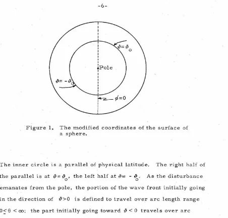
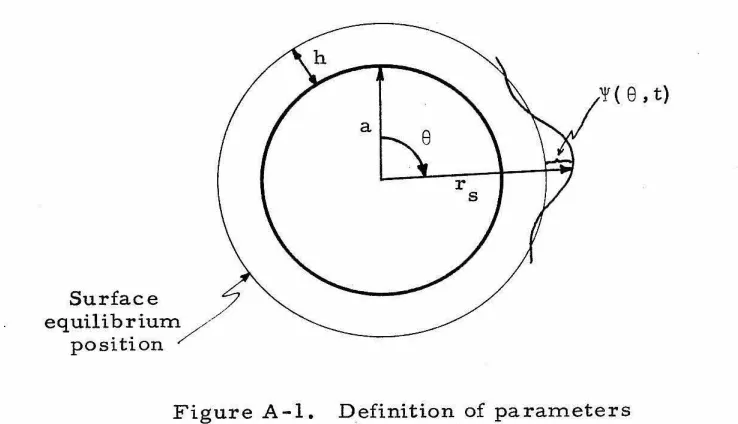
Figure 1. The modified coordinates of the surface of a sphere.

The inner circle is a parallel of physical latitude. The right half of

the parallel is at ~ = ~ ₀ , the left half at ·'1= _.

-

emanates from the pole, the portion of the wave front initially going

in the direction of ~>0 is defined to travel over arc length range

0~ 8 < oo; the part initially going toward ~ < 0 travels over arc

length 0 > 8 > -en.

Using this convention, an observer situated at physical

latitude ~> 0 sees the first pass of the wave front when 8= .J.

The other half of the wave passes him on its first return trip to the

starting pole, at 8 = -2rr

+

on its second journey toward the opposite pole, he sees the portion

the other half meets him at 8= -41T

+

=

fact is of great importance in the analysis of the problems in the following sections. It should be noted that ??-

=

Section 3. The Analytic Continuation of Legendre Functions.

In this section we examine the nature of the solutions of

Legendre's equation (1. 1) defined on the infinite 8-interval. When

this equation is restricted to the customary range 0<

e

two usual notations for the solutions are

w

=

\)-2 and ( 3. 1)

They are called the associated Legendre functions of the first and

second kinds, respectively. We choose degree \) -~ because

pf-L ₁ (cos 8)

\)-z

Qf-L ₁ (cos 8) -\)-2

1s an even function of \)1 ( [ 1], p. 140, (1) ), and

is a solution independent from Qf-L 1 (cos 8). \)-2

To extend these solutions to an infinite 8 interval, one

might be tempted to observe that cos ( 8

+

=

hold that

and

QfJ.

\)-z

+

pf-L J._ (cos ( 8

+

\)-2

=

However, such a direct extension of the solutions is in error. The

notation (3. 1) for the solutions is intended only for the range

[ 0, 1T]. It is well established (see [ 1

J ,

Legendre functions have branch points at 8

=

=

must use another device to bypass the branch points and continue

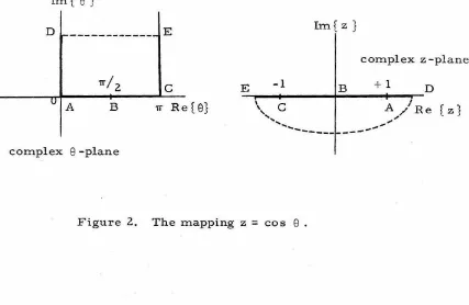
We let 8 be an unrestricted complex variable and

consider the mapping z

=

Im { 8}

--- E Im{ z}

complex z-plane

c

+

B rr· Re{e}

'\.,, c

... ...

_____ _

{z}

complex 8 -plane

Figure 2. The mapping z

=

From this illustration it is apparent that the lower half of the

z-plane ..P m { z}-:: 0 maps onto the upper semi-infinite strip

in the 8-plane: O~Re { 8}-:: 1r; ..Pm {8}:;: 0.

By making the substitution z

=

algebraic form of Legendre's equation:

(3. 2)

This equation is of hypergeometric type. Of the many

choose ( [ 1], pp. 136-137):

. zF 1

[t

+ f.l,

t

+ \) + f.L;

+

+

where 1( C) is the gamma function and

2F 1 [a, b;c;

C

J

=

+

f

+

a(a~f~~l~+l) ~

+ .

.

.

is the hypergeometric series.

Expression (3. 3) has branch points at z

=

(3. 4)

define the branches so that when .,Pm [z} < 0 {3. 3) converges for

..;m [

e}

=

e.

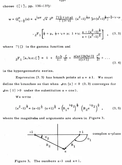
We write

2

~

icp1)~

(

i

cpz)t

=

=

1e R2e , (3. 5)

where the magnitudes and arguments are shown in Figure 3.

-1

+

z

2

As z-0 from any point in the lower half plane, (z -1)--1,

Therefore

( 3. 6)

'lri

1

--z-

and ( z 2 - 1) 2

=

Then if we choose the principal branch of the square root, the

substitution z = cos 8 gives, from (3. 7)'

(z2

-1)~

Making these substitutions in {3. 3) we see that the entire expression

will be a function of 8. Emphasizing that we wish to consider 8

and not cos 8 as the independent variable, the result is

'lrij.L

r<~

+

v

+

r (l+v)

"""r (

.

e stn e .

[

1 l. . . 2i8l

. _{2F 1} 2

+

+

v

+

+

v

,

J

( 3. 9)

The quantity El-L 1 ( 8) is of course equal to Q!-L 1 (cos 8) for 8

v-2 v-~

on the real axis between 0 and 1r. ~'<

*The notation

E~-i

(

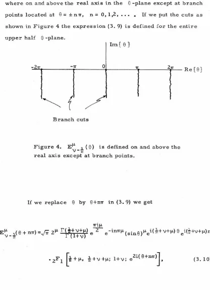
The hypergeometric series in (3. 9) conv.erges every-where on and above the real axis in the 8 -plane except at branch points located at

e

=

=

e

Im{ 8}

-~2~1T4r---~1T ________ 0~,~---~~~---2~1T~-Re{8}

Branch cuts

Figure 4. El-L 1 ( 8) is defined on and above the

\1-z

real axis except at branch points.

If we replace

e

from which we get the important result

E l-l. .(e+n.,.)=l... " ·neinlT\1 El-l. :L (8) , n = ' 0 ±1 ±2 ' , . . . •

\1-z

\1-

z

Equation (3. 11) is the addition formula. It shows directly that the analytic continuation of

oi-L

non-\}-z

periodic. Equation (3. 11) is crucial in the evaluation of integrals occurring later.

One may ask why we chose to extend

oi-L

\)-2

than the more common solution pl-l. ~(cos 8). The reason is that

\1-z

the hypergeometric representations for pl-l. ~(cos e) do not yield

\)

-z-the convenient form of -z-the addition formula (3. 11).

However, it is of interest to examine some form of the continuation of pl-l. 1c (cos 8). There are a number of identities

\1-z

relating the two standard solutions. In particular, from [ 1], p. 140, we have

The substitution z = cos 8, J1rn [z} "'::: 0, and \! _, \!-~ in the above form gives the continuation of the left-hand side and consequently the right side. Thus, we can define

to be the continuation of pf.i. ~(cos 8). Similarly, using V--z

Q~v-1

Q~

we get

e -if.I.TT [

E~

~

E~

t (

J

Another fundamental definition is

(3.13)

E r- (8)-~'IT i e pr- ,(cos8)+

11 eif.i.TT [ iTTV u

V-t

--z

P~ -~

8)]

for

o-:;

r

formula (3. 11) we get the identity

cos VTT pf.i. ~(cos 8), cos TT(V+f.L) v--₂

(3. 15)

O<Re [ 8} ":: 1r.

These relationships are useful for the evaluation of certain integrals. It should be mentioned that while (3. 12) does give the analytic continuation of pf.i. ~(cos 8), it is not especially useful

v

--z

Section 4. Derivation of the Transform.

In this section we derive two forms of the spectral representation associated with (1. 1). Appendix B outlines the theory of constructing the spectral representation associated with an ODE. (For a full treatment of the subject, see Titchmarsh [ 3].)

Starting from (B. 7), we define A.

=

v

-%.

fundamental formula is the contour integral expansion theorem for Dirac's a-function:

=

~

J~(

'ITl 0 v dv

cl

where .1>-(8, 8

0 , v) is the Green's function for (1.1) and

c

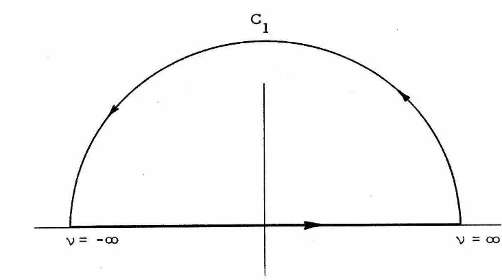
the infinite semicircle shown in Figure 5.

( 4. 1)

v

=

v

In Appendix C one form of the Green's function for (1. 1) is

shown to be

where

,.Bi(8,

e

=

0 .

Ef-1. :L ( 8 ) Ef-1. ₁( 8 ) sin 8 e -2if-l.1T

v-z > -v -2 < o _{( 4. 2)}

are the greater and lesser of 8 and 8 ' respectively.

0

We note that 6( 8 - 8 ) is the value of the integral in (4. 1)

0

taken along the arc

c

1 itself. To get an equivalent representation

for the right -hand side of ( 4. 1), we close the contour

c

1 along the

real axis (Figure 5) and apply Cauchy's integral theorem.

The spectral expansion ( 4. l) becomes

6(8- 8 )=

0 l / 00

- . - ${8, 8 , v) v dv

+

1T 1 0 ( 4. 3)

-oo

By comparing (4. 2) with (3. 9), we observe that the I'-functions in

the denominator of (4. 2) cancel those contributed to the numerator

by the E' s. The factor I' ( l

+

denominator obeys the identity

l ( l

+

=

and is canceled by the remaining factors in v$( 8 I 8 ' v). Therefore

0

the integrand in ( 4. 3) has no singularities, and we get the 6-function

6 (8-8 )

0

i -2ij.L1T

= --

Each side is symmetric in 8 and 8 •

0 Therefore, we can set

8 = 8 and 9> = 9. Multiply each side by f( 8 ) and integrate

< 0 0

from -oo to oo to get the transform pair:

00

£( 9)

=I

f(

-oo

..., i

f(v)=--1T

00

e-2ij.L1T

f

-oo

El-L ~ ( 8) sin 9 d 9 .

-v-~

(4. 4)

( 4. 5)

( 4. 6)

These last two expressions are called the infinite-angle generalized

Mehler transform, after F •. Mehler [ 4] who constructed a

some-what similar transform in connection with the conical functions

P. ~(cos 9).

lV-

z-We can set the order j.L = 0 in (4. 5) and (4. 6). If we define

E0

~

=

~

~

v-~ v-₂ v-₂

transform pair reduces to

00

f(9) = ;

J

Ev-

~

(

9

)

f(v)= -

.i_

J

00

f(9)E

~(

9

)

1T -v-z

-00

( 4. 7)

This special case was derived by Clemmow [2 ] . In some of the

examples that follow it will turn out that ( 4. 7) -( 4. 8) is the

appropriate transform pair to use.

In the special case of the reduced transform, the expansion

of the a-function becomes

6(8- 8 ) =

0

i

- --z

v--z o

Tf

( 4. 9)

We will offer an alternate form of (4. 4)-(4. 6). We can

choose Ef.l

d

v -2 and E-f.l - \)- 2 ~ ( 8) as our independent solutions to

( 1. 1). Appendix C shows that with this pair the Green's function

is

1

=

-sin rr v

( 4. 1 0)

Definition ( 3. 9) implies that the numerator of ( 4. 1 0) contains the

factor

( 4. 11)

and the demoninator contains

1(1

+

=

These factors cancel with others in (4. 10), so there will be no

get the expansion of the 6 -function:

6(8- 8 )=

-~

00

EIJ.

:~J8)

~

o 1r"' v-~ -v-2 o o sin n v

-oo

The resulting transform pair is

1

100,...,

£(

e

= -

~

cos 1T ( V+IJ.) sinrrv

f

.L

fa;(

rr -v-~

-oo

( 4. 13)

dv, ( 4. 14)

Section 5. Application to Waves on a Sphere.

An elegant use of the infinite-angle transform is its

applica-tion to axisymmetric waves on a sphere. The physical problem

selected for study is long free-surface water waves on a shallow

spherical ocean. In Appendix A we show that the linearized

equation for such waves is

si~

8~~

=

where (8, t) is the elevation of the free surface above the eq

uilib-rium position. As explained in Section 2, the variable 9 in (5.1)

can be regarded as the total arc length covered by the wave front,

so -oo

<

<

Equation (5.1) with 0 ~ 9 ~ or has no doubt been solved in

-numerable times using the standard Legendre polynomial expansion.

However, this form of the solution is difficult to analyze or inter

-pret physically. We seek a more transparent expression.

shall examine ( 5.1) with initial conditions

ljJ(S, 0)

=

v₀ ,

jej

lj;t(8,0)

=

<

jej

<

-v 0 ' 1r- 8o

<

\

ej

<

We

(5. 2) (5. 3a)

(5. 3b)

(5. 3c)

These conditions correspond to the sphere's being given an initial

outward velocity throughout a zone at one pole and an identical

inward velocity around the other pole. (This balanced initial

From the pr~nciple of superposition we can treat (5. 3a) and (5. 3c) separately. To illustrate the use of our transform, we will solve the problem with condition (5. 3a) only, stressing that the case with (5. 3c) follows in the identical manner. The conventional form of the solution of (5.1)-(5. 3a) is

~(9, t) = iv₀t(l-cos9_{0 )} +

Vo oo 1

~ n+ 7

c n=l ..fn(n+I)

9o

J

Pn(cos~) sin~ d~

0

• P(cos9)sin{n(n+I)ct.

n ( 5. 5)

It is difficult to interpret (5. 5) directly. For example, it is not at all clear that, for sufficiently small t, ~(9, t)

=

>

then ( 5. 3) implies that the entire sphere is given an initial outward

velocity. It is easily shown that

TT

/Pn(coss) sins ds = 0

0

for n

=

'¥(8,t)

=

0

The entire sphere expands uniformly into space forever. Such

behavior may be at odds with one's intuition, but the result is

( 5. 6)

correct for the very simple physical system which equation (5. 1)

describes. )

We will now extract the solution of (5.1)-(5. 3a) using the

infinite-angle transform. From ( 4. 9) and ( 4. 1 0), define

and

1(8,t)

=+

~~

-oo

'l' ( v' t) = sin

e

{ 5. 7)

( 5. 8)

Multiply (5. 1) by i E l ( 8) sin 8 and integrate from

rr

-v-

The first integral in ( 5. 9) can be integrated by parts:

1

ae

00

. 00

(sin8~~)

=sine~@

E_'V_i(8)1--co

00

-

f

o'¥ .

ae

e

-00

We assume '¥(8,t) and '¥

8(8,t)-0 as 8-±CD. Therefore, the boundary term in (5. 10) vanishes and we get

CD

f

~ ~

°

'V-~(

°

-~(8)1

00

+

-CD

-CD

( 5. 9)

(5. 10)

(5.11)

Now E _{-v -2} 1 ( 8) is a solution to Legendre's equation (1. 1) with f-1.=0, so (5. 12) becomes

(5.13)

Appealing to (5. 8), this becomes

( 5. 14)

Transforming the initial conditions (5. 2) and (5. 3) gives

·~(v,O)=O

. Je

- - v E

d£)

-rr o -v-2

- 8 0

It follows that

~(v,t) = sin£d£· ( 5. 15)

and the inverse transform (4. 7) yields the solution

v cot -rr v d v .

This solves (5. 1) - (5. 3) for -oo < 8 < oo. Interchange the order of integration and rearrange terms to get

8 00 _ _ _..,

v o

i

sinV} -

i

'!' (

e

,

=

ds·

- L

- 8 rr -oo ~I 2 1

0

"v

-

E _

v

_

(

s)

v

_

(

s

v

v

v.

( 5. 1 7)

As stated before, the variable 8 in (5. 17) represents total arc length, measured from the starting pole, covered by the wave. In Section 2 we showed that the disturbance ~ ( ~?, t) observed at physical latitude

(} is the sum of the individual disturbances at arc lengths (}

+ 2nrr,

n

=

00

qi ( (}, t) x

2:

+

or

qi ( (} ' t)

OJ

J

=

0

dsf

sin~

v

-i

c _n-

~

v

2

0 ' 4•

( 5. 18)

oo

je

H~.

=

L (

e

d~

~

,-..---..

. 2 ~ 2.

s1n \1 - 4 ct 1nrrv e

n= -oo o

(5.19)

The \1 -integral in (5. 19) has the structure of a Fourier transform.

We will evaluate it using the convolution theorem for Fourier

integrals. Let F(\1) be the Fourier transform of f(a.):

1/

-1 \)a.

F(v)= ₂rr f(a.) e do..

-<X>

If G( \1) is the Fourier transform of g( a.), then the convolution

theorem states that

00 00

I

=

2

~

j

-oo -oo

(5. 20)

Define F( \1)

-.•

r;-;_

smlv""-i ct.

~

\)

2

-i

(5. 21)

Then, from [ 6] , p. 26. (30). we find that

(5.22)

where I (z) is the modified Bessel function of the first kind, order

zero, and H(x) is the Heaviside unit function' H(x)

=

~~:

~;~

Define G( v) - - (

1

> )

E _-v-2 1 (~) E _{v -2} dt?) sin~ v cotrrv dv (5. 23)

Fror:n the ()-function expansion (4.13) and the addition formula (3.11)

we get the representation

i/

6(??

+

(5. 24)

Let a.= 4nrr and each side of (5. 24) is a function of a.. We get the

Fourier formula

1

eia.v

.I-~)

1

(~)

~(??)sin~

o(t?+cx.-~).

00 \" rr - v-2 v -2

(5. 25)

From the results in (5. 22) and (5. 25) we will use the convolution

formula (5. 20) to determine the v-integral in (5. 19).

00

1

00

Evaluating the integrand at the zero of the a-function argument yields

'H~.

t)

~

[2;

-l)nf

8

\

0

[~~t

2

-

(,Hz:;-S>zJ

H(ct-

J

~+Zntt-5!)

df;.

0

(5. 26)

For any finite t this expression contains only a finite number

of terms, each one representing a separate passage of the wave front

around the sphere. We shall analyze the behavior of the wave.

From the symmetry of the physical problem the solution

must be symmetric in rJ. Therefore, we will consider the

behavior seen by an observer at latitude rJ >0.

Case 1. rJ > 8 .

0

In this situation the observer is located outside the zone

of initial velocity. We examine H ( ct -

I

+

g

I)

The argument first becomes positive in the n

=

0

The integration variable ~ is confined to (-8 , 8 ) , and hence

0 0

il>(.,,t) - 0 for t<

"-8

This fact shows directly that the initial wavefront travels with speed

c into a quiescent medium and that there is no advance disturbance.

After the wave front first arrives the expression (5. 26)becornes

rJ-8

0

- -

2rr- rJ-8

0

c

where A is the algebraically lesser of -8 and {)- ct. This

0 0

expression represents the first passage of the initial wave front.

Now, I {z) is bounded near the origin. Its appearance in the

0

integrand of {5. 27) implies that the surface level rises continuously

and monotonically from zero for the time interval specified

in {5. 27).

This behavior shows that the wave propagation on the

sphere is not "clean-cut" but leaves an infinitely long wake.

At time

t

=

2rr-{)-8

0

c

the n=-1 term q>_

1{{), t) in {5. 26) appears. It represents the first

return trip of the wave front to the starting pole. In the interval

<

<

c

the total disturbance is

v q> { {). t)=

2~

2rr+{)-8

0

c

I

₀

~ ~t

2

_(.?-:~-")Jd"

Here A ₀ is defined as for { 5. 2 7), and A _

1 is the algebraically

smaller of 8

0 and {)+ct -2rr. The disturbance obeys this formulation

until

2rr + {) - 8

t= _ _ _ _ _ -o

c at which time the n= 1 term q>l { {), t) appears

(5.29)

where Al l S the algebraically lesser of - eo and {)-

+

The next two terms to enter are then= -2 and n = 2 terms,

respectively. From the factor ( -l)n in (5. 26) it is evident that

successive pairs of terms are alternately positive and negative.

This fact has the remarkable interpretation of a phase reversal

occurring at the far pole but not at the starting pole. ~ , the

. 0

initial wave coming from the starting pole, is positive. The

contribution from ~-l, the first return from the far pole, is

negative. The term \P

1, representing the second pass from the

starting pole, is also negative, indicating no change of sign.

The second return wave ~ ~

2

of sign at the far pole.

Case 2. {)- < 8 .

0

The observer here is situated within the zone of initial

velocity. Rather than evaluate ( 5. 26) directly we make the

following observation. The single initial condition ( 5. 3) can be

written as the swn of the two conditions

·where

(5.30)

and f₂(

e

= -

e

<

l·.e I

<

0 0 . - (5. 32)

This corresponds physically to our combining the solutions to separate initial-value problems: one in which the entire sphere

receives an initial outward velocity, and one where the zone now under consideration is initially quiet while the remainder of the sphere is given an inward velocity -v .

0

It follows either from (5, 5) or directly from (5. 1) and (5. 2)

that, with condition (5. 31) as the initial velocity,

q> (t?,t)

=

0 ( 5. 33)

When we include (5. 32) as our initial velocity distribution,

the~; except for a change in coordinate limits, we have precisely the physical problem of Ca~e 1 above. Making the necessary adjustments in the notation of (5. 26), we can combine the separate solutions to the problems using (5. 31) and (5. 32) individually to get

211"-8

<!(-' •

t):

t'

~~ ~:(

- l ) t

\

[

~

t

2

_(-'+Z:n-g)

2

]H(ct-1

-'+2nn-g

~

as the solution to our original problem (5. 1)-(5. 3) with t?< 8 •

0

( 5. 34)

We shall analyze (5. 34) for the first few moments of wave travel. For

8 -t?

t

<

the series contributes nothing, and

= v t

0 •

a uniform outward motion. At

8 -{}

t = 0 c

the n=O term <P ({},t) entersandweget

0

<P ( {} • t) = v t

0

8 -{} 8 +?'J _o __ < t < _o _ _

c c

(5.35)

where A is the lesser of ~

+

0 0

represents the propagation of the effects of initial quiescence from

the nearer boundary of the initial disturbance inward to the observer's

latitude.

t

=

At

8 +{}

0

c

the n = 1 term appears. It can be interpreted as the arrival of

quiescence effects from the far boundary of the initial disturbance.

As in Case 1, (5. 34) admits more and more terms as t

increases. However, we must make the distinction that (5. 34)

describes the disturbance in terms of the propagation of quiescence

effects, whereas (5. 26) represents the acutal disturbance itself.

Thus, we find that while the physical wave undergoes a phase reversal

at the far pole, the quiescence terms encounter such a change only

Propagation Of An Explosion.

Of particular interest is a special case of the above problem representing the behavior of the sphere following a point explosion at one pole. We reduce the size of the zone

I

e

I

e

0

increase the velocity v

0 in such a way that the total initial energy

remains constant as

e

.... o.

0

We define the initial energy per unit area to be the total energy E: exhibited by initial condition (5. 3) is

0

so,

2

e

0

=

e

>,

v

=

0

1

- cos

e

0

Substitute (5. 36) into the solution (5. 26) to get

q, ( t<i ' t) =

rc

1 ...

1 -;;-J

re;;

-==1====->: ( -1)

,:.

nf

e·

.

o

1 -cos

e

e

Applying the mean value theorem for integrals and expanding

"h

e

0

in a power series for

e

0

Then

(5.36)

1

~

r;:

g)( t?' t)

=

-f

where - 8 < 8 < 8 .

0 1 0

Take the limit of (5. 38) as 8 -+ 0 to yield

0

( t?+2mr -

8

1

~

. 2 8 .

0

c

( 5. 3 8)

It? +2mr

1)

as the representation for the disturbance at any physical latitude t?

resulting from an explosion at the starting pole at t = 0. It· reveals

quite clearly the behavior of the wave.

The first contribution again comes from the n

=

factor H(ct-t?) shows that there is no disturbance at t? before

t

=

c

Now I (0)

=

0

surface elevation jumps abruptly to height

t?

1~

~(t?. - )

= -

c c 1T

As the wave proceeds, the surface at t? continues to rise

2•rr- !?-In the interval

c

q>(t?-,t)

<

<

t?-+2rr

The n

=

=

the wave on its second trip toward the far pole.

Because of the infinite initial velocity at one pole it is

worthwhile to examine the wave for possible subsequent singularities

at either pole. From (5. 39), there is no disturbance for t < ~ .

The first wave contributes

'lr 3rr

c

<

<

We see that, although the radial velocity of the wave front changes

abruptly with the arrival of the wave, the amplitude remains bounded

and has no physical singularity. From (5 .. 39) we deduce that similar

Section 6. The Flow of Heat on a Spherical Shell.

In this section we derive an alternative representation for

an axisymmetric initial-value heat-flow problem on a spherical

shell. The standard form of the heat diffusion equation is

2

k'V u - u = O t

We consider an initial distribution of temperature over a zone. Equation (6. 1) becomes

si~

~~)

- at

au

=

with initial condition u( 8,

o>

0 ,

I

I

<

Classically, the eigenfunction expression in terms of Legendre

polynomials yields

00

u( 8, t)

=L

n n

n=O

with the result

( 6. 1)

(6. 2)

(6. 3)

P(cos8)· n

-n(n+l) kt

e .

This equation is useful for large kt. The total heat remains constant, and the temperature tends to a uniform distribution over the entire sphere.

For small kt the series in (6. 4) is· slowly convergent. To get a more rapidly convergent form, we define 8 to be arc length on the sphere and hence -oo

<

<

of heat in an initial-value problem resembles an infinitely fast,

exponentially weak wave. Therefore, we follow Section 2 and note that the temperature U { t?, t) at physical latitude {1 is

00

U( '!?, t)

=L.:

Now we shall solve {6. 2)-{6. 3). Multiply

(6.

i.._

1T -\)-2

and integrate from - oo to oo.

( 6. 6)

From the exponential decay of the solution to the heat

equation in an infinite domain we assume u{ 8, t) _,Q for 8--+ ± oo.

Therefore when we integrate the first term in (6. 6) by parts twice

-

~

k1:

e

+

~~= ~~

=

( 6.

E ~( 8) satisfies (1. 1) with tJ.

=

-\)-2

<X>

8 d 8

+

l_l

d

= 0.

(6. 8)

Each term here has the form of the infinite-angle transform ( 4. 15 ),

so (6. 8) becomes

'"" 2~,..., )

ut(v, t)

+

-·:d

=

Transforming the initial condition (6. 3) solves (6. 9):

I

e

,..., i 1-.kt 0

u (

v,

= - -

f

~

~)

1T 0 \ )

--

e

0

sin ; d ;

~

The inverse transform (4. 14) gives

2

-\) kt

e

(6. 9)

Equation ( 6. 9) gives the temperature at any arc length 8. To

calculate the result at physical latitude iJ, we appeal to (6. 5);

this expression, together with the addition formula (3. 11) and

interchanging the order of integration, gives

It is well known that

f

-v~

t

e e v

=

-(X)

E \J _

t

(

2

a

- 4kt

e

(6. 1 0)

(6. 11)

Incorporating (6. 11) and (5. 25) into the convolution theorem, we

get

2

ei2nTTV e -v kt E ~ (s) Ev_.1.(iJ) sins v cot TTV dv =

-v-2 :;>

(2 - 4kt

e 0 ( ?.?+ 2nTT -

C

.., S)

C

ikt co

le

u e o

U(

~,

=

~

"'""' (

2 'ITkt ~

n=-co -

e

0

e

2

(!~+2n'IT -~)

4 kt

We shall analyze the behavior of the temperature U{ {}, t).

Case 1. {} >8 .

0

( 6. 12)

For kt sufficiently small the n=-0 term dominates all others because of the rapid decay of the exponential in the integrand. (It also dominates the factor

~

'ITkt

or

U( {}, t) ~

u

0

U(t'l,t) ~

-

,;;-We can write this as

u

u (-{},

-f

{}+ 8

0

l,_ktf

2Jkt

e4 .

19-e

d ~ '

ei kt

(E

E

fh)) .

Case 2. {)< 8 . 0

In this case the observer is situated within the zone of

initial temperature u • As with the wave problem of the previous

0

section we treat this case as the superposition of separate

problems, one with initial condition

and the other with initial condition

u

2 ( 8, O)

=

<

I

I<

The solution to

(6.

u

0

( 6.

(6.15)

(6. 16)

We can solve (6. 2) and (6. 15) by a change in the integral limits

in

(6.

U( .,'), t)

=

0

u e

0

%k.t

21T'-8

L

n= -co o

e

Here again, for sufficiently small kt, the n=O term dominates, and

(

.;hkt 21T'-8 o

U(.,'}, t)

~

4

-

r

o

2..,r;kt.J

e

0

2 - (£-.,'))

Section 7. The Potential of a Sphere.

In this section we apply the generalized transform to obtain an alternative representation for the electrostatic or gravitational potential of a sphere.

We solve Laplace's equation in spherical coordinates:

+

si~

~~)

+

v

=

cpq> (7. 1)

0 2

8 s1n

with boundary conditions

V(a, 8, lfl) = f(8,qJ), 0 < 8 < rr, 0 <CD < 2rr ( 7 0 2)

lim r

v (

r-+OO

We specify that -oo <8,q> <oo in (?.!).Laplace's equation is one of static equilibriUJ;n, so we cannot interpret the solution as the contribution from a traveling disturbance. Because lfl as well as

e occupies an infinite range, we must now distinguish between the extended azimuth

cp

c/

J

cj

observer. The total potential at physical point (r, {},

¢)

+

¢

+

=

1 !2'11"

:('IT

~

V(r,

8

,q>)=

2

'1T(~)

d~

.

d

C

sinCf(

C

,~L

· o o n=O

n

m=-n

a n

For r> >a the factor ( -) implies that the series is rapidly

r

(7. 4)

convergent. The first few terms give a good approximation to the

actual potential.

For r ~a we would require an inconvenient number of

terms for accurate d~scription of the potential, since ( ~ )~ 1s

no longer dominant. This fact,for instance, hampers concise

calculation of the gravity force on a spacecraft orbiting a planet.

We will use the Mehler transform to derive a representation useful

for r~ a.

We define the Fourier transform

g

Take the Fourier transform of (7. 1). The boundary terms arising

from the integration by parts of the last term vanish, leaving

2- - 1

a

r

v

-8

<=>

e

rr r s1n u

(

.

.

e

oV

f.L~

_L

e

)

Sln (}

e

.

e

Multiply ( 7. 6) by i E-JJ. de) sine

'IT - v-~ and integrate over e

from -oo to oo. We integrate the third term by parts. The boundary terms again vanish and we get

f

i 2 -jJ.

- - r · V ( r, e, JJ.) E ~ ( e)

'IT _

00

00

v(r,e,JJ.).

'IT r

-oo

sin _{e d 8}

-n:-

as

a (

aeE-~-

a _

~

(

8

)

)

./00

+

'IT

-oo

2

iJ. V( r 8 n) E-JJ. " ( 8) d 8 = 0 .

sine ' ...

-v-t

( 7. 7)

With the aid of Legendre's equation (1. 1) we can simplify the third and fourth integrals; combining terms in the resulting expression gives

= 0 •

(7. 8)

From the Mehler transform formula (4. 15) we define

. /00

'l'(r, v, JJ.)

=-

V

-oo . -v-2 sin e de. ( 7. 9)

whose solution is

'¥ = A( v, !J.) r

v

-

.J..

+

(v,

-v-

i

,..._ / c o i!J.cp

V(r, 8, !J.)

=

-oo

Boundary condition (7. 3) implies

lim ra V(r, 8, q>)

=

r--eo

which together with (7. 12) gives

lim ra V(r, S,iJ.)

=

hnposing (7.13) on (7.9), we get.

lim ra'l:'(r, v, !J.) = 0 for a < 1 • r->oo

Therefore, the solution (7. 11) becomes

'¥ ( r, v, !J.)

=

A(

v,

v,

v

-.J..

r 2

r -v-~

-~ <v<~

(7.10)

(7.11)

(7.12)

(7. 13)

By transforming initial condition (7. 3) and inverting (7. 12) and

(7. 9) we find the result

sin r ~ v ---:---'----!..."'-cosrr(v+f.L) H (

I I

v -

) \

)

sin rr v C

'(7. 15)

where H(x) is the Heaviside unit function.

This expression is the potential at the extended coordinates 8 and

cp. The total physical potential iJ.i(r,,9,¢') is given by

(X) (X)

iJ.i(r,?J,¢')

=L

L

m= -co n= -co

From the addition formula (3. 11} we get

S l n r ~\) cosrr( . Vl-f.L)

s ln 1T \)

(7.16)

We first evaluate the v -integral in (7. 16). Recalling the

i E-1-1 (r) El-L (")sin r \) cos'l!" ('V+IJ.)

- -z -

i

"'

'II"

=

2i1? 2F 1 [ . . . e

J.

(7.17)

Integrate both sides of (7. 1 7) over \) from -oo to co. The left-hand side is just the 6 -function expansion (4. 13). Therefore

( 7. 18)

where C( 8, C ,IJ., 'V} represents the remaining factors on the right-hand side of (7. 17).

Another well-known expansion is i'V("-C) 1 d e

""""2ir

( Subtracting (7. 19} from (7. 18) we obtain that

1

C(1?, C ,IJ., 'V)

=

2'iT

and hence

(7. 20)

N as

or

Let N standforthe v-integralin(7.16). Wecanwri.te

N= 2 \ J

(~)l

v

l

-oo

1 00 \)

N=-J

(~)

or ~ r .

2

The result is

N=..!__/i(-l}n or~r

log(~) cos i (?J-C)- (?Jt2nrr-i.:)sin-t(?J-C)

2 2

[log(~)] + [~ + 2nor-CJ

There is no f.L-dependence in this integral, so we can do the

f.L-integral in (7. 16} to give

foodf.Le-if.l(~

-ro

(7.21)

Now O<s< 2or, so the only contribution to (7. 16) from (7. 21) is for

m= 0. Therefore ourfinal result is

00

rr . !log(2:.)cos-t(tJ-C)-(?.?+2nrr-C)sini(?J-C)

~

(r,?.?,¢')=-1 (~)""-"

J

rr

rL.J

n=-oo [log (a)

J

J

d (

This representation for the potential is superior to the

usual expression (7. 4). In modern applications (7. 4) has been

used extensively in the calculation of the gravitational force of a

celestial body on a nearby spacecraft. Not only do we have to

calculate a double integral numerically, but also for r ~ a several

dozen terms in the double series are required for a good

approx-imation to the potential. Unfortunately, the calculation of such a

large number of associated Legendre functions poses serious

num-erical problems.

In (7.22) we have the advantage of having to evaluate only

a single integral and series. Even more significantly, we need

only sines and cosines and avoid completely the computation of

PART II

Sound Waves in the Ocean

Section 8. Introduction.

We shall derive the spectral representation associated with the DE

w _,,

+ [ "'

2 (

1

+

.

M ) -A]

0

(

c. cosh2 (tmz)

00

and apply it to solve the PDE modeling the propagation of sound waves in the ocean. The spectrum is found to be mixed, requiring both an integral and a series to constitute the complete

representation.

Equation (8.1) arises from the separation of variables method applied to the linear wave equation with variable sound speed. In Section 9 we start with the PDE and derive the

Section 9. Derivation of the Spectral Representation.

A problem of interest is the propagation of small-amplitude

sound waves in the ocean. It has been widely determined

experimentally that the speed of sound in the oceans of the earth

is non-uniform. There is a decided minimum speed at a depth

of roughly 1200 meters, with a sharp increase above and below it.

The depth of minimum speed is called the sound channel.

The far field in the vicinity of the channel shows prominently the

trapping and focusing effects caused by the non-uniform sound

speed when a point source is located in the channel.

There has been substantial investigation of the steady- state

case of this problem, using a variety of models for the variation of

sound speed with depth. (For an extensive bibliography, see the

paper by Deavenport [9].) Blum and Cohen [8] investigated the

initial-value problem, where the source begins emitting sound at

time t

=

representation to an asymptotically more convenient form by a

Watson contour integration. One of our aims is to derive the

exact expression for this form using a new spectral representation.

For simplicity we consider an ocean of infinite extent in all

directions with a vertical variation of sound speed. Because of the

horizontal uniformity we express our problem in cylindrical

coordinates, with the origin in the channel and the z -axis directed

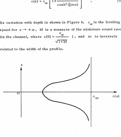
speed c(z):

c(z)

=

-Yz

[

1+ M

cosh2 (tmz)

]

Its variation with depth is shown in Figure 6.

( 9.1)

c is the limiting 00

speed for z - ± oo, M is a measure of the minimum sound speed

c

00 (in the charmel, where c(O) =

---Jl+M

related to the width of the profile.

z

) , and m is inversely

c c( z)

(X)

The initial-value problem we study using speed (9.1) is

p (r,z,t)+-p (r,z,t)+p 1 (r,z,t) 1 [ 1+--~;__ M __

J

rr r r zz c: cosh2 H·mz)

= -

/Tr

o~r)

(9.2)

-oo

<

<

<

<

<

p(r, z, 0)

=

(9.4)

p(r, z, t) - 0 and outgoing waves

(9.5)

as r-oo, z - ± oo.

The quantity p(r, z, t) is the observed deviation at point (r, z) from

the ambient pressure. This problem represents a point source at

radius r

=

=

according to f(t) beginning at time t

=

We separate variables in the homogeneous form of (9. 2):

_R"

+l-R\~"-

[l +--::.:.M=---]

2 1

c

00 cosh2 (-zmz)

T"

Til

Define

T

= -

Fourier transform. Equation (9.6) becomes

R 11 _{1 R} 1 _Z 11 _w2

- + - - + - + -

0()

[

1+

M

J

cosh2 _(-~mz)

=

The terms are separately functions of r and z. Define

and the equation for Z yields

z

=

Z"

+

[

1

+

coshz (tmz)

It can be easily shown that two solutions of (9.8) are

(9.7)

(9.8)

Z

=

=

V-72 V-72

where

V"'(t+4

M)

~

w

cZmZ

0()

(9.10)

and

~"'~(\

)

~

(Principal Branch)

--cZ

0()

By imposing the outgoing wave condition (9.5) we construct the Green's function

{j

q

(z, z_{0 ,} f.l(\))

= -

· r

(t

+

v

+

r

<i -

v

+

where z> and z< are the greater and lesser of z and z₀ ,

respectively.

(9.12)

Now we can apply the fundamental spectral formula (B.7):

o(z - z_{0 )}

=

2

~

s

q

+

l

CB A. -plane). (9.13)

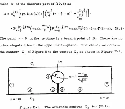
From (9.11) and (9.12) we see that the point fJ.

=

convergence of the solutions at z

=

m2 w2

Therefore we make the change of variable A. =

4

+-cz

00

ioo

>--=

>-.-plane f.L- plane

(a) (b)

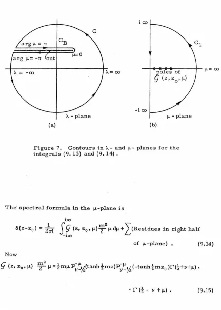
Figure 7. Contours in>-.- and f.L- planes for the

integrals (9. 13) and (9. 14).

The· spectral formula in the f.L-plane is

ioo

O(z-zo)

=

}rri

s

~

f.L)~

2

f.LdJJ.+ l(Residues in right half

-100

of f.L -plane) • (9.14)

Now

The function p-IJ._{1 ;} {~) is an entire function of IJ.. In

V-72.

Appendix E we show that

v

that there are simple poles from the r-functions at 1-L =

1

-

n = 0 , 1 , ••• , N , where N is the largest integer less than

lv 1-

~.

The o-function expansion (9.14) becomes

· r

v

I-n) •

Multiply each side of (9.16) by f{z_{0 )} and integrate over z₀ from

-oci to oo. The resulting transform pair is ioo

f{ z)

=

S

f

~z)

v

-v

n*l-!

+

L

f

(~~)n P;!~~-~)+n

~z)

{I

vi-~

where 00

f

=

S

f{z)P;~

Yz

~z)

-oo

and

00

- ms

fn

=

T

f(z)P-(l~j-Yz)+n(-tanh

For any fixed ll this spectral representation contains an integral

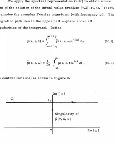
Section 10. Application to Sound Waves in the Ocean.

We apply the spectral representation (9.17) to obtain a new form of the solution of the initial-value problem (9.2)-(9.5). First, we employ the complex Fourier transform (with frequency w ). The integration path lies in the upper half w-plane above all

singularities of the integrand. Define

oo+i'Y

S

'

-

=

-oo

+

00

- 1

p(r, z, w)

=

271'

S

iwt p(r, z, t)e dt •

-oo

The contour for (10.1) is shown in Figure 8.

i

0

Im [ w}

Singularity of p(r,z, w)

Figure 8. Integration path for (10. 1).

Re[w}

(10.1)

00

We define F(w)

= -

i1T

S

0

transforms to

[

1+ M

coshz (imz) ]

- ..§J.!l

p = Z1rr c5{z-z₀ )F(w).

{10.3)

Now we apply the transform (9.17)-{9.19). Multiply {10.3) by

P~~Yz

~z)

Equation {10. 3) becomes

[ 1+ _{coshz (imz)} M p-IJ.ll/

v-

( -tanh

~zo

From {9.5) it follows that p, pz' - 0 as z - ± oo.

Therefore, we can integrate the third term on the left in {10.4) by parts twice and the boundary terms vanish. Combining this result with the fact that

P;~Vz

~z)

{9.8),

( (

~rr +~ ~r

+

(~

2

- ..§itl.

1; (-tanh m₂z 0 ₎

- 27Tr v-72 (10. 5)

From (9.18) we define

00

~

S

p

w)~"!Yz

~z

=

which yields from (10.5)

1 (mZ wZ ) im -f.L (

mzo)

t/J

+-1/J

-

t/J

-rr r r 4 z

8 z v-72 2

c 1T

00

.2J.!.l

r . (10. 7)

We recognize (10. 7) as the zero-order Bessel equation. Its solution obeying the outgoing wave condition with time factor

-iwt

H~

)

(z) is the Hankel function of the first kind, and

sgn (x)

=

1

-1,

x<O

x>O

To get the full representation for p(r, z, w) (and consequently for

p(r, z, t) ), (9.17) implies that we must have a contribution lf; (r, w)

n

from the discrete spectrum. It is derived precisely as lf; (r, f.L, w).

It is shown in Appendix E that we can translate the w-contour down

to the real axis in the discrete spectrum. The variable v is real

for real w, so the inverse transforms (9.17) and (10.1) give the final

result

oo+i"Y

S

p(r, z, t)

=

-oo+ i "Y

oo

nivi-Yz

[

im -iwt -1 n 1

+s

S_:we

~

H~

Yz

• p-(!v!-Yz)+n (-tanh mzo)

v-Yz

p-(!v!-

v-Yz

~z

!v

· r

I

v

1-

This expression represents the complete disturbance observed at any point (r, z} with the source located at (0, z₀ }. We shall analyze certain aspects of this result.

When the source and receiver are both far above the channel it is apparent from Figure 6 that the surrounding speed is nearly uniform. Therefore, the corresponding solution will not differ significantly from a pure spherical wave.

The behavior of the solution in the vicinity of the channel is more complex. (The variation of sound speed throughout the actual oceans of the earth compares quite favorably with the central portion of the Epstein profile.} By performing a Watson transformation on the Hankel representation of p(r, z, t) ,

Blum and Cohen ( 8] obtained an expression for the case

z = z₀ = 0 (source and receiver in the channel) asymptotically valid for r - oo. We can reduce expression (10.8) to theirs i f

we ignore the continuous spectrum , set z

=

=

not n clean-cut"- they have tails or wakes that tend to obscure

It is known [8] that the continuous spectrum in (10.8) is

0 (

~

o(;.. )

=

=

(10.8) becomes

· <!vi -

t-

r (

From

[1],

fJ. _ 1 ( 1

+

)Yz

p

v

r

+v,

-

v'

t -t

from which (10. 9) becomes, after interchanging summation and

integration,

00 00

p(r,z,t) ....

,i~

l S

H~

)[••••]P~~~~-l/z)+n(O)·

1

r<t

+

•F(!+v,!-v;!+lvl-n; 1 )

_!!!, (

lvl-~-

I

l+emz {10.10)

For mz << 1 , each of the integrals in the series is reduced by a factor

-

~ <!vi-~-

e Because of the exponential the

high-frequency components of F{w) will be drastically attenuated,

even at a small distance from the channel. The implication is that if

the forcing function f{t) at the source is a sharp pulse, the

dominant behavior just outside the channel will be a smooth rise and

long decay. Thus, long distance, high frequency communication is

APPENDIX A

Derivation of the Equation for Waves on a Sphere

We shall derive the equation for the axisymmetric free-surface

water waves on a shallow ocean covering a solid sphere. For

in-viscid, incompressible, irrotational fluids the fundamental equations

are

Continuity:

\1·

Momentum: "'i'\7'"t

au

+

=

where u

=

+

+

of fluid, F is the vector sum of external forces, p is the constant

density, and p is the local pressure. The symbol

\1

operator, and \lu is a dyadic appropriate to spherical coordinates.

In the simplest approximation we ignore the non-linear term

u • \lu. For axisymmetric waves there is no azimuth dependence and

a - o

aq;

= •

(A. 3)

which can be written as

(A. 4)

In the momentum equation we assume that the only external force is

gravity and that it is constant throughout the depth of the ocean. Then

and (A. 2) reduces to the pair of equations

au

a t

=-g-p8r

ap

1

ap

p;a-e

(A. 6)