Theory and simulation of passive scalar mixing in the presence of a mean scalar gradient

(1)

the Presence of a Mean Scalar Gradient

Thesis by

Paul O’Gorman

In Partial Fulfillment of the Requirements for the Degree of

Doctor of Philosophy

1 8 9 1

C A L

IF

O

RN

IA

IN STI T U

T E_{O F}

T

E C

H

N

O

L

O

G

Y

California Institute of Technology Pasadena, California

2004

(2)

c

° 2004

(3)

Acknowledgements

Studying and performing research at Caltech was a rewarding and pleasant experience for me. I would like to thank my advisor, Dale Pullin, for making this possible, and providing the necessary guidance and encouragement. Almost all the work for this thesis was carried out in the Iris lab, and so I thank my friends who worked there for the range of conversation and strange debates that made it easy to come to work each day.

A special mention goes to my housemates at 201 South Michigan, where we stayed for four years, despite heat, cold, and poor cleaning. The last year has been extra fun thanks to Rosie and Cathy.

I would like to thank my parents, Ambrose and Imelda, and my sister Mary. They provided a good perspective on what is important in life, and have supported me well at each turning point.

(4)

Abstract

The turbulent mixing of a passive scalar in the presence of a mean scalar gradient was investigated using theory and simulation. The velocity-scalar cospectrum measures the distribution of the mean scalar flux across scales. An inequality is shown to bound the magnitude of the cospectrum in terms of the shell-summed energy and scalar spectra. At high Schmidt number this bound limits the possible contribution of the sub-Kolmogorov scales to the scalar flux. At low Schmidt number we use an argument of Batchelor, Howells, and Townsend (1959) to derive a new asymptotic result for the cospectrum in the inertial-diffusive range, with a −11/3 power law wavenumber dependence. A comparison is made with results from large-eddy simulation at low Schmidt number.

The sparse direct-interaction perturbation (SDIP) was used to calculate the cospec-trum for a range of Schmidt numbers. The Kolmogorov type scaling result is recovered in the inertial-convective range, and the constant of proportionality was calculated. At high Schmidt numbers, the cospectrum is found to decay exponentially in the viscous-convective range, and at low Schmidt numbers the −11/3 power law is ob-served in the inertial-diffusive range. The stretched-spiral vortex model was used to calculate the cospectrum, and asymptotic expressions were found for the contribu-tion to the cospectrum from the axial velocity in the vortex structures. Results are reported for the cospectrum from a direct numerical simulation at a Taylor Reynolds number of 265, and a comparison is made of results for the cospectrum from the SDIP, the stretched-spiral vortex model, simulation, and experiment.

(5)

(6)

List of Figures

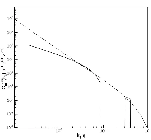
2.1 Comparison of the scalar spectrum from the LES (solid) and the low Schmidt number asymptotic form given by equation (2.36). . . 21 2.2 Comparison of the velocity-scalar cospectrum from the LES (solid) and

the low Schmidt number asymptotic form given by equation (2.31). . 21 2.3 Comparison of the energy spectrum from the LES (solid) and inertial

range form given by equation (2.30). . . 22 2.4 Schematic representation of the winding of the axial velocity in a vortex

structure. Scalar variations in the axial direction are in turn distorted by the axial velocity. . . 26 2.5 Schematic representation of a stretched vortex structure and the mean

scalar gradient. . . 29 2.6 The 1D cospectrum contributed by the axial velocity from the

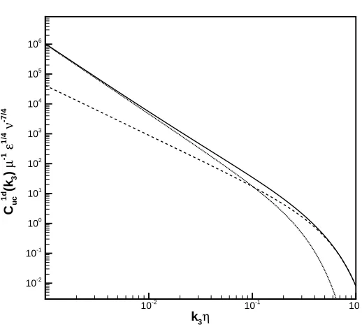
stretched-spiral vortex model. Dashed, -5/3 component. Dotted, -7/3 compo-nent. Solid, both components. . . 42 2.7 Comparison of the 1D cospectrum contributed by the axial velocity

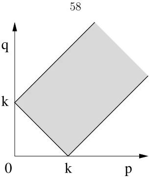
and the planar velocity from the stretched-spiral vortex model. Solid, planar contribution. Dashed, axial contribution. . . 43 2.8 Integration region used in the SDIP integrals, denoted by 4k. . . 58

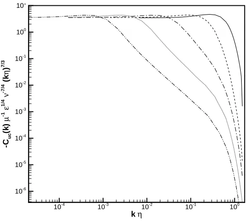
2.9 SDIP results for the compensated shell-summed velocity-scalar cospec-trum at Schmidt numbers 1 (solid), 2 (dashed), 10 (dotted), and 100 (dash-dotted). . . 64 2.10 SDIP results for the compensated shell-summed velocity-scalar

(9)

2.11 SDIP results for the compensated shell-summed velocity-scalar cospec-trum at low Schmidt numbers (same key as Figure 2.10). Here the wavenumber has been normalized with the Obukhov-Corrsin wavenum-ber, and the thick solid line shows the inertial-diffusive asymptotic result given by equation (2.31). . . 67 2.12 SDIP result for the compensated shell-summed velocity-scalar

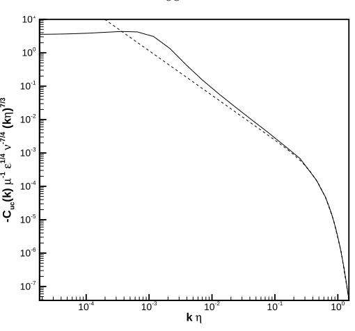
cospec-trum at Schmidt number 10−4 (solid) compared with the SDIP asymp-totic form given by equation (2.210) (dashed). . . 68 2.13 SDIP results for the shell-summed velocity-scalar cospectrum

(uncom-pensated) at Schmidt numbers 10−4 (dashed), 1 (solid), and 104 (dot-ted). The power laws k−7/3 _and _k−11/3 _{are also shown for reference. .} ₆₉

2.14 Cross-section of the total scalar field with 5122 gridpoints, including the mean gradient in the horizontal direction. The scalar values are normalized as (c+µ x₁)/(µ l). . . 72 2.15 Isosurfaces of the vorticity magnitude and the scalar fluctuation. The

volume shown is 1/64 of the compuational domain. (a) Isosurface of the magnitude of the vorticity, at a value three standard deviations above the mean value. (b) Isosurfaces of the scalar fluctuation at c/(µ l) of

−2.0 (yellow), 0.0 (green), 2.0 (blue). . . 73 2.16 Spectra from the DNS at 5123 (full line) and 2563 (dashed line): (a)

energy spectra in compensated form, (b) scalar spectra compared with

k−5/3, and the stretched-spiral vortex result from reference [40] (dotted line). . . 75 2.17 (a) Velocity-scalar cospectra from the DNS at 5123 (full line) and 2563

(dashed line) compared with a k−7/3 _{power law. (b) Velocity-scalar}

(10)

2.18 Comparison of compensated one-dimensional velocity-scalar cospectra from the stretched-spiral vortex model (dashed), experimental data from reference [34] at Rλ = 582 (solid), DNS at Rλ = 265

(dash-dot-dot), SDIP inertial-convective (dotted), and SDIP (dash-dot). . . 78

3.1 (a) ˇR(k, σ) and (b) ˇRc₍_{k, σ}_{) for ¯}_k _{= 200 from the stretched-spiral}

vortex model with stationary vortex structure centers; numerical eval-uation (full line), asymptotic evaleval-uation (dashed line). . . 91 3.2 (a) ˇR(k, σ) and (b) ˇRc(k, σ) for ¯k = 3000 from the stretched-spiral

vortex model with stationary vortex structure centers; numerical eval-uation (full line), asymptotic evaleval-uation (dashed line). . . 92 3.3 Energy spectrum from the non-axisymmetric vorticity for the

stretched-spiral vortex model. . . 93 3.4 DNS results for the modal correlation function of (a) the velocity, and

(b) the scalar: ¤ kη = 0.0087, 4kη = 0.0137,O kη = 0.0216, ♦ kη = 0.0341,

◦

kη = 0.0538, ¥ kη = 0.0848, N kη = 0.134, H kη = 0.211, ¨

kη = 0.332,

•

kη = 0.524. . . 96 3.5 DNS results for the modal correlation function of (a) the velocity, and

(b) the scalar using the sweeping time scaling. See Figure 6 for the key to the symbols used. . . 97 3.6 DNS results for the modal correlation function of (a) the velocity, and

(b) the scalar using the inertial time scaling. See Figure 6 for the key to the symbols used. . . 98 3.7 Comparison of DNS results for the modal time correlation function

of the velocity (full line) and the scalar (dashed line) using the same wavenumbers as in Figure 6. . . 99 3.8 R(k, σ) at (a) kη = 0.0848, and (b) kη = 0.211: DNS results

•

,

(11)

3.9 Rc₍_{k, σ}_{) at (a)} _kη _{= 0}_._{0848, and (b)} _kη _{= 0}_._{211: DNS results}

•

_,

stretched-spiral vortex model (full line). Also shown are exp(−k2u2_rmsσ2/2) (dash-dotted line), and ˇRc

(12)

List of Tables

(13)

Chapter 1

Introduction

The problem of turbulent passive scalar mixing shares many of the features of the classical turbulence problem, and has important applications in areas such as turbu-lent combustion and dispersion in geophysical flows. A passive scalar is a contaminant in a fluid that has no dynamical effect on the fluid itself, for example, temperature in the case of a weakly heated flow. The scalar field evolves under the combined influence of molecular diffusion and advection by the velocity field, according to the advection-diffusion equation. Although this equation is linear in the scalar, predicting the statistics of the scalar field is nonetheless a difficult problem. The canonical prob-lem for passive scalar mixing involves mixing by an incompressible turbulent velocity field in the presence of a uniform mean scalar gradient. The velocity field is assumed to be statistically homogeneous and isotropic, and it can then be shown that the mean scalar gradient is preserved by the evolution of the flow. This problem has been the subject of extensive study because the mean gradient acts as a source of scalar variance, allowing a statistical steady state to be reached, see Overholt and Pope [37]. The mean gradient makes the problem non-isotropic, however, and so a mean scalar flux arises. The statistics of the scalar field show many similarities to that of the ve-locity field, but the mean scalar gradient also leads to some interesting difference, for example, anisotropy at small scales due to ‘ramp-cliff’ structures in the scalar field, see the review by Warhaft [48]. Here we will concentrate on two particular statistics; the velocity-scalar cospectrum, and the Eulerian modal time correlation functions. The velocity-scalar cospectrum represents the distribution of the mean scalar flux across scales, and the modal time correlation functions can be used to determine the characteristic timescales for the high wavenumber modes of the velocity and scalar fields.

(14)

scalar flux is given by

u₁c=

Z _∞

0

Cu1c(k)dk, (1.1)

where c is the scalar fluctuation, u₁ is the component of velocity in the direction of the mean scalar gradient,kis the wavenumber, and the overbar indicates an ensemble average. Thus the velocity-scalar cospectrum gives the distribution of the mean scalar flux across scales, making it relevant, for example, to problems in turbulent heat transfer. A mean scalar flux can only occur as a result of anisotropy, and so it is interesting to know how quickly the cospectrum decays with increasing wavenumber. If, as is thought, the cospectrum decays faster than the scalar or energy spectra, then this is a measure of the approach to isotropy at the smaller scales. In addition, because the total scalar flux represents transport in the scalar advection-diffusion equation, knowledge of the cospectral properties of vortex-models is expected to be useful in their application to the building of subgrid scalar-flux and mixing models for use in large-eddy simulation [38]. Also of interest is the effect of the Schmidt number on the cospectrum, and hence the scalar flux, where the Schmidt number is defined as the ratio of viscosity to the scalar diffusivity. The effect of Schmidt number on the scalar spectrum is still the subject of ongoing research, for example, the experimental work of Miller and Dimotakis [31] at high Reynolds number, and the simulation by Yeung et al. [50] at low Reynolds number.

While considering the effect of buoyancy on the energy spectrum, Lumley [28] used a similarity hypothesis to predict the shell-summed cospectrum of the velocity and potential temperature in the inertial-convective range. If the gravitational force is set to zero, then the absolute and potential temperatures are the same, and Lumley’s equation (12) for the cospectrum simplifies to

Cu1c(k)∼µ ²1/3k−7/3, (1.2)

(15)

cospectrum depends only on k, ²and µ.

Mydlarski and Warhaft [34] studied the velocity-temperature cospectrum in a wind tunnel for Taylor Reynolds numbers, Rλ, as high as 582. Fluctuations in the passive

temperature field were generated by imposing a linear mean temperature gradient across the tunnel. The resulting cospectrum was noisier than the energy or scalar spectra, and this was explained by noting that no mathematical limitation keeps the spectrum either positive or negative. Nonetheless, they found a wavenumber dependence of approximately k−2 in the inertial-convective range for Rλ of 582, see

also [33]. Interestingly this would represent a slower approach to isotropy at the small scales than the Lumley scaling result (1.2). Of course, the experimental exponent may indeed approach−7/3 for higher Reynolds number, but the variation in the exponent over the range ofRλ reported by Mydlarski and Warhaft [34] seems to asymptote to

an exponent closer to−2.

Kaimalet al. [20] measured the cospectra of velocity and potential temperature in the atmospheric surface layer, see also Wyngaard and Cot´e [49]. They found that the cospectrum involving the horizontal velocity showed a k−5/2 scaling range, and the cospectrum involving the vertical velocity showed ak−7/3 _{scaling range. We mention}

these results for completeness, although of course the surface layer is significantly different from the simpler mixing case we consider here.

There have been few attempts to calculate the velocity-scalar cospectrum using either theory or simulation. Herr, Wang and Collins [17] performed an EDQNM calculation of the cospectrum, and compared it with direct numerical simulation (DNS) at anRλ of 81, although it should be noted that two constants were chosen in

the EDQNM calculation by matching the EDQNM and DNS cospectra.

We turn now from the velocity-scalar cospectrum to two-point, two-time statis-tics of the velocity and scalar fields. A fundamental, but still disputed property of isotropic, homogeneous turbulence is the characteristic timescale over which the small scales of the velocity field decorrelate in an Eulerian frame of reference. Kolmogorov scaling in the inertial range suggests the inertial eddy-turnover time, (²k2)−1/3_{. There}

(16)

where urms is the root-mean-square (rms) velocity [45, 36, 16, 22, 25]. Knowledge of

the correct time scaling would be useful, for example, as an input to the recent func-tional derivative closure (FDC) [12] for random advection of a passive scalar, and in interpreting the importance of the random sweeping effect [45]. Also of interest is the characteristic timescale of the small scales of a passive scalar mixed by a turbulent velocity field.

The velocity modal time correlations are the time correlations of the Fourier modes of the velocity field, and so are a two-time, two-point statistic. Several attempts have been made to use characteristic time scalings to collapse these correlations to a universal form. The main experimental work is by Comte-Bellot and Corrsin [6] in decaying grid turbulence, and is at a maximumRλ of 72. They achieved a collapse of

the modal time correlations using a parallel combination of four different characteristic timescales. DNS studies by Orszag and Patterson [36] at Rλ ∼ 16, Gotoh et al. [16]

at Rλ ∼ 46, Kaneda et al. [22] at Rλ ∼ 126, and Sanada and Shanmugasundaram

[45] at Rλ ∼200, all found the ‘sweeping’ timescale to be dominant.

Kraichnan [25] studied the modal time correlation and made a simple linearized estimate, and also an estimate based on the direct interaction approximation (DIA), both of which resulted in the ‘sweeping’ time being the characteristic timescale. Mc-Comb et al. [30] studied numerical solutions to the DIA and local energy trans-fer (LET) theories, and in contrast to Kraichnan’s asymptotic prediction for the DIA, found that while neither the ‘sweeping’ timescale nor the inertial eddy-turnover timescale were completely effective in collapsing the modal time-correlation data, the inertial scaling became more dominant for both theories as Rλ was increased.

Fi-nally, Gotohet al. [16] studied the modal time correlation using both DNS and DIA at Rλ ∼ 35, and found that the sweeping timescale gave a poor collapse of the

cor-relation data from the DIA relative to the data from the DNS. In contrast to the velocity modal time correlation function, the scalar modal time correlation function has received little attention.

(17)

overall aim is to study the velocity-scalar cospectrum and modal time correlation functions using a combination of theory and direct numerical simulation (DNS). It is of interest to use approaches that have been shown to provide quantitative results for the velocity statistics to problems involving a passive scalar, one example being the recent use of the stretched spiral-vortex model to calculate the scalar spectrum [40] for homogeneous but non-isotropic turbulence. Here we will work with two notable theories that are successful in linking the Navier-Stokes equations and the Kolmogorov phenomenology, namely, the stretched-spiral vortex model introduced by Lundgren [29], and a Lagrangian reformulation of the direct-interaction approximation (DIA) of Kraichnan [25].

The stretched spiral-vortex model of turbulence uses an ensemble of vortex tubes to model the fine scales of turbulence. The vortex tubes do not interact except in that they are stretched on average by the surrounding flow. The vortex tubes are assumed to be straight, with no dependence of the velocity field on the coordinate parallel to the tube axis. In each tube the vorticity is evolved by the Navier Stokes equations and the scalar is evolved by the advection-diffusion equation. The axial vorticity, the axial velocity, and the scalar are each wound up into spirals by the differential rotation of the cores of the vortices. Average flow statistics are calculated by performing an average over time and space. This model gives good results for energy [29] and scalar spectra [40] individually. By also performing an average over vortex orientation the model was used to calculate vorticity and velocity-derivative moments [41], as well as one-dimensional spectra [42]. Here we will use the model to calculate the velocity-scalar cospectrum, as well as modal time correlation functions of the velocity and scalar fields.

(18)

ap-plied in an Eulerian frame of reference, the resulting equations are not consistent with the Kolmogorov form for the energy spectrum in the inertial range. However, there are several Lagrangian reformulations of the DIA without this property, one example being the sparse direct-interaction perturbation (SDIP), first introduced by Kida and Goto [24] with the name Lagrangian direct-interaction approximation. It is a renormalized closure theory for second-order turbulent statistics that applies a similar procedure to Kraichnan’s direct-interaction approximation (DIA) [25] in a Lagrangian framework. The SDIP is simpler than the Lagrangian history DIA of Kraichnan [26], and yields the same integro-differential equations as the Lagrangian renormalized approximation (LRA) of Kaneda [21]. The SDIP has been used to cal-culate the energy spectrum [24], and the scalar spectrum [14]. Goto and Kida [15] applied the SDIP to a simpler dynamical model to better understand the basis of the approximation. In light of the importance of sparse coupling in the approxi-mation, the name sparse direct-interaction perturbation was then chosen in place of Lagrangian direct-interaction approximation. Here, we will use the SDIP to calculate the velocity-scalar cospectrum. One advantage that the SDIP has over simulation and experiment is the relative ease with which the cospectrum can be calculated for a range of different Schmidt numbers.

To complement the above calculations we performed a DNS of turbulent mixing of a passive scalar with a resolution of 5123 gridpoints. There have been a number of numerical passive scalar mixing studies at comparable resolution, see Overholt and Pope [37], or Yeung et al. [50]. Comparison with box turbulence simulations at higher resolution but with no passive scalar suggest that at this resolution we can expect to capture the beginning of the inertial range, see Kaneda et al. [23]. One advantage of DNS is the ease with which different statistics can be calculated, and here we report results for the velocity-scalar cospectrum, as well as the modal time correlation functions of the velocity and scalar fields.

(19)

(20)

Chapter 2

The Velocity-Scalar

Cospectrum

Throughout this chapter we will consider a passive scalar mixed by an incompressible, statistically homogeneous and isotropic velocity field, ui(x, t). The scalar is assumed

to have a mean scalar gradient, µ, in the 1 direction, so that we can decompose the scalar as µ x₁ +c(x, t). The scalar fluctuation c(x, t) is statistically homogeneous, and axisymmetric about the x₁ axis, but not isotropic. By definition it has zero mean, c(x, t) = 0, where the overbar indicates an ensemble average. If we define the velocity-scalar correlation by

Ruic(r) = ui(x, t)c(x+r, t), (2.1)

then the shell-summed velocity-scalar cospectrum is defined by

Cuic(k) =

1 (2π)3

Z

S

Z

V

Ruic(r)e−ik·rdrdSk, (2.2)

where the S integral is a surface integral over a spherical shell in wavenumber space, and theV integral is a volume integral over all space. The shell-summed cospectrum has no imaginary part, as may be seen by rewriting the shell integral as an integral over a hemisphere, _Z

S

e−ik·rdSk = 2

Z

Sh

cos(k·r)dS_kh, (2.3)

and it integrates to the scalar flux,

uic=

Z _∞

0

(21)

The shell-summed cospectrum is thus a measure of the distribution of the scalar flux across scales.

One-dimensional spectra are often more convenient for experimental measurement, and so we define the one-dimensional velocity-scalar cross spectrum by

F_u1_iD_c(k₃) = 1 2π

Z _∞

−∞Ruic

(0,0, r₃)e−ik3r3_dr

3. (2.5)

In general the cross spectrum may be complex, and can be split into real and imagi-nary parts as

2F_u1_iD_c(k₃) = C_u1D_i_c(k₃)−i Q1_uD_i_c(k₃), (2.6)

where C_u1_iD_c(k₃) is the cospectrum and Q1_uD_i_c(k₃) is the quadrature spectrum [3]. The integral of the one-dimensional cospectrum over all wavenumbers is also equal to the scalar flux,

uic=

Z _∞

0

C_u1_iD_c(k₃)dk₃. (2.7)

The quadrature spectrum is related to phase differences between the Fourier compo-nents of the scalar and the velocity fields. In Appendix A the quadrature spectrum is shown to be zero for the case of isotropic incompressible turbulence and a mean scalar gradient. It is also shown that only the cospectrum of the scalar and the ve-locity component in the direction of the mean scalar gradient is non-zero, where this holds for both the shell-summed and one-dimensional cospectra.

(22)

Schmidt number asymptotic forms for the velocity-scalar cospectrum and the scalar spectrum are compared with results from a large-eddy simulation.

In section 2.2 the cospectrum is calculated using the stretched-spiral vortex model. The mean scalar gradient is held fixed, while the isotropic turbulent velocity field is modeled using vortex tubes oriented with equal probability in all directions. For the velocity field provided by the stretched-spiral vortex, the velocity-scalar cospectrum can be divided into two additive components contributed by the velocity components along the vortex axis, and in the plane normal to this axis, respectively. For the axial velocity field, a new exact solution of the scalar advection-diffusion equation is found exhibiting scalar variation in the direction of the vortex tube axis, allowing the scalar evolution to be influenced by the axial velocity. This is important because the scalar and the axial velocity evolve in a similar way, unlike the scalar and a given planar component of the velocity, and leads to an important contribution to the velocity-scalar correlation. An asymptotic expression is found for the cospectrum contributed by this solution and the axial velocity, with the leading order term showing a k−5/3

range. This term is produced by the winding of the initial axial velocity field by the axisymmetric vortex core. The next-order term gives a k−7/3 _{range, and arises}

from the lowest order effect of the non-axisymmetric vorticity on the evolution of the axial velocity. Its coefficient can be of either sign or zero depending on the initial conditions. The contribution to the cospectrum from the velocity in the plane of the vortex is also calculated, but no universal high wavenumber asymptotic form is found. The integrals are evaluated numerically and it is found that the the resulting cospectrum does not remain of one sign. Its form depends on the choice of the vortex core velocity profile and time cutoff in the spectral integrals.

In section 2.3 the sparse direct-interaction approximation of Kida and Goto [24] is used to calculate the cospectrum. In the inertial-convective range the Lumley form µ ²1/3_k−7/3 _{is recovered, and the constant of proportionality is calculated. The}

(23)

derived, appropriate for wavenumbers in the inertial-diffusive and viscous-diffusive wavenumber ranges. This form agrees with the asymptotic result of section 2.1 in the inertial-diffusive range.

In section 2.4 we describe a DNS of turbulent passive scalar mixing, performed at a Taylor Reynolds number of 265, and a Schmidt number of 0.7. Results are reported for the cospectrum, and these are compared with the bound given by the cospectrum inequality.

Finally, in section 2.5 we make a comparison between the results for the cospec-trum from the stretched-spiral vortex model, the SDIP, the experiment of Mydlarski and Warhaft [34], and our DNS.

2.1

The cospectrum at small and large Schmidt

numbers

(24)

inertial-diffusive range with results from a large-eddy simulation.

2.1.1

The cospectrum inequality

Here we will derive an upper bound for the magnitude of the shell-summed velocity-scalar cospectrum in terms of the energy and velocity-scalar spectra. This bound has close ties to the one-dimensional cross-spectrum inequality and coherence function, discussed in Bendat and Piersol [3]. In effect, we are extending the one-dimensional cross-spectrum inequality to the three-dimensional shell-summed case, and applying it in particular to the velocity-scalar cospectrum.

It is convenient to use the formulation of the SDIP calculation in section 2.3, where we first work in a periodic box of side L, and then take the limitL→ ∞. For consistency, we also adopt the convention used in that section for denoting integrals, where the associated infinitesimal is placed beside the integration sign.

The velocity field ui(x, t) can be decomposed as

ui(x, t) =

µ

2π L

¶₃ _X

k ˜

ui(k, t) exp(ik·x), (2.8)

where ki = 2π ni/L, and ni ∈Z. The inverse Fourier transform is given by

˜

ui(k, t) =

µ

1 2π

¶₃ Z

d3xui(x, t) exp(−ik·x), (2.9)

and a similar transformation is defined for the scalar fluctuation, c(x, t). We then define the second order statistical quantities

˜

Vij(k, t, t) =

µ

2π L

¶3 ˜

ui(k, t) ˜uj(−k, t), (2.10)

˜

Z(k, t, t) =

µ

2π L

¶₃

˜

c(k, t) ˜c(−k, t), (2.11)

˜

Wi(k, t, t) =

µ

2π L

¶₃

˜

(25)

The double reference to the time t is included to be consistent with the definition of more complicated Lagrangian quantities in section 2.3.

For a given instance in the ensemble, we have that

Re(˜c(k, t) ˜u₁(−k, t))≤ |˜c(k, t)| |u˜₁(k, t)|, (2.13)

where we have used that ˜u(−k, t) = ˜u(k, t)∗. Taking an ensemble average we find that

Re

³

˜

c(k, t) ˜u₁(−k, t)

´

≤ |c˜(k, t)| |u˜₁(k, t)| ≤

³

|c˜(k, t)|2 |u˜₁(k, t)|2

´1/2

. (2.14)

The second inequality can be derived by considering the expression

(|˜c(k, t)|+ξ|u˜₁(k, t)|)2, (2.15)

as a quadratic in the real numberξ, and requiring that it be non-negative.

Taking the limit L → ∞ we can relate ˜Vij(k, t, t), ˜Z(k, t, t), and ˜Wi(k, t, t) to

power spectral density functions. The shell-summed energy spectrum, E(k), scalar spectrum, Ec(k), and velocity-scalar cospectrum, Cu₁c(k), are given by

E(k) = 1 2

Z

dSkV˜ii(k, t, t), (2.16)

Ec(k) =

Z

dSkZ˜(k, t, t), (2.17)

Cu₁c(k) =

Z

dSkW˜1(k, t, t), (2.18)

whereR dSk denotes a surface integral over a shell in wavenumber space, rather than

a solid angle integration. We will now use the fact that the shell-summed cospec-trum is real. This can be seen from equation (2.18), and the relation ˜W₁(k, t, t) =

˜

(26)

E(k)/(6πk2), we deduce the inequality

Cu₁c(k)≤

1

k

µZ

dSkZ˜(k, t, t)1/2

¶ µ

E(k) 6π

¶1/2

. (2.19)

Similarly we can show that inequality (2.19) holds for −Cu1c(k), and so it also holds

for the magnitude |Cu₁c(k)|. The scalar spectrum is anisotropic, and so we cannot

perform the solid angle integration without further knowledge of ˜Z(k, t, t). Nonethe-less, we can find a bound in terms of the shell-summed scalar spectrum. Using the Cauchy-Schwartz inequality we have that

Z

dSkZ˜(k, t, t)1/211/2 ≤

µZ

dSkZ˜(k, t, t)

¶₁/2 µZ

dSk

¶₁/2

=¡4π k2Ec(k)

¢₁/₂

,

(2.20)

and so,

|Cu₁c(k)| ≤

µ

2E(k)Ec(k)

3

¶1/2

. (2.21)

It should be noted that a tighter bound might be deduced with more detailed knowl-edge of the scalar anisotropy.

2.1.2

Implications of the bound

From (2.21) we see that the magnitude of the cospectrum is bounded by the geometric mean of the scalar and energy spectra multiplied by a constant of order unity. To discuss the implications of this, we first briefly review the phenomenology of the scalar spectrum at different Schmidt numbers.

We assume in what follows that the Reynolds number is sufficiently large for an inertial-convective range to exist. The Schmidt number is defined as the ratio of the viscosity to the diffusivity,Sc =ν/D. We definekP as the wavenumber at the peak of

the energy spectrum or the scalar spectrum, whichever wavenumber is greater. The Kolmogorov wavenumber is defined by kK = (²/ν3)1/4, the Batchelor wavenumber

(27)

given bykC = (²/D3)1/4 =Sc3/4kK. Then for wavenumbers in the inertial-convective

range the scalar spectrum has the form

Ec(k)∝ ²c²−1/3k−5/3, kP ¿k ¿min(kK, kC), (2.22)

where²c is the scalar dissipation, and the constant of proportionality is known as the

Obukhov-Corrsin constant, see Tennekes and Lumley [46]. For large Schmidt number a different power law behavior is thought to exist in the viscous-convective range [1],

Ec(k)∝ ²cν1/2²−1/2k−1, kK ¿k ¿kB, ScÀ1. (2.23)

For very small Schmidt number, in the inertial-diffusive range,

Ec(k)∝ ²cD−3²2/3k−17/3

µ

1 + 2D µ 2

²c

¶

, kC ¿k ¿kK, Sc¿1. (2.24)

We show this in subsection 2.1.4 by modifying a result of Batchelor, Howells, and Townsend [2] for the presence of a mean scalar gradient. There are other theoretical predictions for the scalar spectrum in this range, for example, Gibson [11] found ak−3

wavenumber dependence. Finally, in the viscous-diffusive range the scalar spectrum decays exponentially.

Now consider the velocity-scalar cospectrum for the case of large Schmidt number in the viscous-convective range. According to (2.23) the scalar spectrum has a k−1

wavenumber dependence, whereas the energy spectrum will be decaying exponentially with wavenumber because k À kK. Therefore, the bound given by inequality (2.21)

(28)

this should be apparent in a comparison between the mean scalar profile for mixing layer flows at different Schmidt numbers, see Dimotakis [7] for a review of free shear layer mixing in gases and liquids.

In contrast, for the case of small Schmidt number in the inertial-diffusive range, the scalar spectrum has a wavenumber dependence of k−17/3 _{according to (2.24), the}

energy spectrum has a k−5/3 wavenumber dependence because kP ¿ k ¿ kK, and

so the bound given by inequality (2.21) has a k−11/3 _{dependence. Therefore, in this}

wavenumber range we do not necessarily have reason to expect exponential or power law behavior of the cospectrum based on the inequality. However we will be able to derive an asymptotic form for the inertial-diffusive range in subsection 2.1.3.

In subsection 2.3.6 the SDIP is used to solve for the cospectrum at a range of Schmidt numbers, and a comparison is made of the resulting cospectra with the bounds given by (2.21).

2.1.3

Asymptotic form in the inertial-diffusive range

We consider the case of low Schmidt number, and wavenumbers in the inertial-diffusive range, kC ¿ k ¿ kK. The advection-diffusion equation for the scalar

fluctuation is given by

∂

∂tc(x, t) +uj(x, t) ∂ ∂xj

c(x, t) =D ∂

2

∂xj∂xj

c(x, t)−µ u₁(x, t), (2.25)

where we note the gradient forcing term. This can be written in Fourier space as

·

∂

∂t+D k

2

¸

˜

c(k, t) = −µu˜₁(k, t)−i

µ

2π L

¶₃ _X

q

qju˜j(k−q, t) ˜c(q, t). (2.26)

Following the argument of Batchelor, Howells, and Townsend [2] we note that the convolution sum in equation (2.26) is dominated by wavenumbers qsmaller thankC,

that is |q| < kC. This is justified because the scalar spectrum drops off rapidly for

higher wavenumbers. Then assuming that k À kC, implies that |k−q| ' k. We

(29)

˜

c(k, t). This can be seen in the case of ˜uj(k−q, t) by comparing the inertial timescale

²−1/3k−2/3 with the diffusive timescale D−1k−2 and usingkÀkC. Therefore, we can

make a stationary balance approximation, and neglect the time derivative in equation (2.26). Multiplying byu₁(−k, t), taking an ensemble average, and using the definition of ˜Wi(k, t, t) (2.12) we find

˜

W₁(k, t, t) =− µ

D k2

µ

2π L

¶₃

˜

u₁(−k, t) ˜u₁(k, t)

− i

D k2

µ

2π L

¶₆ _X

q

qju˜j(k−q, t) ˜c(q, t) ˜u1(−k, t).

(2.27)

We have already argued that |q| ¿ |k−q| 'k, and so we make the further approx-imation that ˜c(q, t) is statistically independent of ˜uj(k−q, t) and ˜u1(−k, t). The

mean ˜c(q, t) is zero, and so

˜

W₁(k, t, t) = − µ

D k2

˜

V₁₁(k, t, t). (2.28)

Taking the limit L → ∞, and using (2.16) and (2.18) to make contact with shell-summed spectra we find

Cu₁c(k) =−

2µ

3D k2 E(k). (2.29)

The wavenumber k is in the inertial range, and so

E(k) = K ²2/3k−5/3, (2.30)

where K is the Kolmogorov constant, with the result,

Cu1c(k) =−

2µ K

3D k −11/₃

²2/3. (2.31)

Thus the cospectrum has ak−11/3 _{power law wavenumber dependence in the}

(30)

mean scalar gradient on the scalar spectrum in the inertial-diffusive range, and this will be the subject of the next subsection.

2.1.4

Effect of the scalar gradient on the scalar spectrum in

the inertial-diffusive range

Here we will see how the Batchelor, Howells, and Townsend [2] result for the scalar spectrum is modified by the presence of a mean scalar gradient. Chasnov [5] studied the scalar spectrum in the inertial-diffusive range using large-eddy simulation (LES), and noted that the Batchelor result [2] for the scalar spectrum is still valid in the presence of a mean scalar gradient when the scalar dissipation is replaced by ²c +

2D µ2. Here we will confirm this using a direct rederivation of the result, taking into account the mean scalar gradient.

In the inertial-diffusive range we have already shown that an approximate equation for ˜c(k, t) is given by neglecting the time derivative in equation (2.26). Multiplying by a similar expression for ˜c(−k, t), and taking an ensemble average gives

˜

c(k, t) ˜c(−k, t)D2k4 =µ2u˜₁(k, t) ˜u₁(−k, t)

− µ

2π L

¶6 _X

p

X

q

pjqiu˜j(−k−p, t) ˜ui(k−q, t) ˜c(p, t) ˜c(q, t)

+i µ

µ

2π L

¶₃ _X

q

qiu˜i(k−q, t) ˜c(q, t) ˜u1(k, t).

(2.32)

Again using |q| ¿ k, |p| ¿ k, and assuming the statistical independence of modes at wavenumberq orp with modes at k−q, k, or k−p, we find

˜

c(k, t) ˜c(−k, t)D2k4 =µ2u˜₁(k, t) ˜u₁(−k, t)

− µ

2π L

¶6 _X

p

X

q

pjqiu˜j(−k−p, t) ˜ui(k−q, t) ˜c(p, t)˜c(q, t).

(31)

This may be simplified to

D2k4Z˜(k, t, t) = µ2V˜₁₁(k, t, t) + ˜V₁₁(k, t, t)

µ

2π L

¶₃_X

q

qjqjZ˜(q, t, t). (2.34)

The sum overq can be related to the scalar dissipation, and taking the limitL→ ∞

and performing a surface integral in wavenumbers space leads to

Ec(k) =

2

3E(k)D

−2_k−4 ³_µ2₊ ²c

2D

´

. (2.35)

We are in the inertial range, and so using the appropriate form of the energy spectrum (2.30) we find

Ec(k) =

1 3D

−3_{K ²}2/3_²

ck−17/3

µ

1 + 2D µ 2

²c

¶

. (2.36)

Equation (2.36) reduces to the Batchelor, Howells, and Townsend [2] result when the mean scalar gradientµis set to zero. Thus the effect of the mean scalar gradient is to change the magnitude of the scalar spectrum, but not its wavenumber dependence. As Chasnov [5] noted, the effect of the mean scalar gradient can be captured by replacing the scalar dissipation with ²c + 2D µ2 in the original Batchelor, Howells,

and Townsend [2] result. We have performed an LES using a different subgrid model to the one used by Chasnov [5], and we will compare with our results for the scalar spectrum and velocity-scalar cospectrum in the next subsection.

We are now in a position to compare our asymptotic result for the cospectrum in the inertial-diffusive range with the bound given by the cospectrum inequality. Substituting (2.30) and (2.36) into (2.21) we find

|Cu1c(k)| ≤

2 3µ K ²

2/₃

k−11/3D−1

µ

²c

2D µ2 + 1

¶₁/2

. (2.37)

(32)

2.1.5

Large-eddy simulation at low Schmidt number

We performed a large-eddy simulation (LES) to verify the asymptotic results (2.31) and (2.36) for the velocity-scalar cospectrum and scalar spectrum at low Schmidt number in the inertial-diffusive range. Our simulation is similar to the LES of Chasnov [5]. Chasnov made a comparison with the asymptotic form (2.36) for the scalar spectrum, and found excellent agreement in the far inertial-diffusive range, but the agreement in the near inertial-diffusive range was not as good. As was the case for Chasnov, we do not need a subgrid model for the scalar because we resolve the diffusive range, but our subgrid model for the velocity is different from that used by Chasnov.

The LES was performed with 643 gridpoints, at a Taylor Reynolds number of 1500, and a Schmidt number of 2×10−4. A statistically stationary state was reached by forcing the velocity at the low wavenumbers using the same forcing scheme as is described in section 2.4, and a mean scalar gradient acted as the source for the scalar variance. Statistics were collected over thirty large-eddy turnover times, and time-averaged spectra are reported.

We used the stretched-vortex SGS model of Misra and Pullin [32], with vortex alignment according to the locally resolved strain rates (model 1a), and a spiral-vortex type energy spectrum at the subgrid scales. Evaluation of the second-order velocity structure function was used to calculate the subgrid energy, see Voelkl et al. [47] and Pullin [38] for further details. This LES method has the advantage of dynamically giving a value for the Kolmogorov constant, which we then use in expressions (2.31) and (2.36).

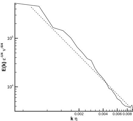
The LES result for the scalar spectrum, and the asymptotic result given by (2.36) are compared in Figure 2.1. The Obukhov-Corrsin wavenumber corresponds to kCη '0.002, and so we can see that in the inertial-diffusive range the agreement

(33)

kη Ec

(k

)

ε

3/

4 ν

-5

/4

εc

-1

0.002 0.004 0.006 0.008 101

102 103

104

105

Figure 2.1: Comparison of the scalar spectrum from the LES (solid) and the low Schmidt number asymptotic form given by equation (2.36).

kη

-C

uc

(k

)

µ

-1

ε

1/

4 ν

-7

/4

0.002 0.004 0.006 0.008 104

105

106

107

(34)

kη

E(

k

)

ε

-1

/4

ν

-5

/4

0.002 0.004 0.006 0.008 104

105

Figure 2.3: Comparison of the energy spectrum from the LES (solid) and inertial range form given by equation (2.30).

than the LES result. Thus, LES seems to confirm both asymptotic results for the velocity-scalar cospectrum and the scalar spectrum, although of course any mech-anism that requires a resolved viscous range has been neglected in our LES. For reference, we show in Figure 2.3 the energy spectrum from the LES compared with the inertial-range form (2.30), where we have again used the Kolmogorov constant given by the LES.

2.2

Application of the stretched-spiral vortex model

(35)

choice of initial conditions. The contribution from the axial velocity is evaluated us-ing its asymptotic form for high wavenumber, but the contribution from the velocity in the plane of the vortex can only be evaluated numerically.

2.2.1

Evolution of scalar and velocity fields in a stretched

vortex tube

We wish to find the evolution of the velocity and scalar fields in a vortex tube em-bedded in a background linear velocity field. It will be important in this section to distinguish between lab and vortex fixed frames, because the mean scalar gradient is assumed to be fixed with respect to the laboratory frame. Therefore, we adopt a temporary notation, wherexiare vortex fixed axes, andx0iare laboratory coordinates.

The vortex fixed coordinate, x₃, is aligned with the vortex tube axis. The velocity field of the vortex tube is assumed independent of x₃, but may have a component in the direction of the vortex axis. The scalar is in general a function of all three spatial coordinates. The following analysis generalizes that of Pullin and Lundgren [40], hereafter referred to as PL, by letting the scalar have an x₃ dependence. The effect of this change on the scalar spectrum is discussed in Appendix B.

It will be convenient for the moment to work with the total scalar field ct(x, t) =

µ x0₁+c(x, t), rather than the scalar fluctuation c(x, t). The Navier-Stokes equations for the velocity ui and the vorticityωi are

∂ui

∂t +uj ∂ui

∂xj

=−∂π

∂xi

+ν∇2ui, (2.38)

∂ωi

∂t +uj ∂ωi

∂xj

=ωj

∂ui

∂xj

+ν∇2ωi, (2.39)

and the advection-diffusion equation for the scalar ct₍_x

1, x2, x3, t) is

∂ct ∂t +uj

∂ct ∂xj

=D∇2ct, (2.40)

(36)

The velocity field is decomposed as

ui =vi(x1, x2, t) +ai(t)xi, (2.41)

with a₁ +a₂ +a₃ = 0 and a₃ > a₂ > a₁. Summation over i is not implied. If the support of the vorticity is compact in a domain surrounding x₁ = x₂ = 0 then the velocity can be expressed in terms of a vector potentialψi(x1, x2, t) as

v₁ = ∂ψ3

∂x₂, v2 =− ∂ψ₃

∂x₁, v3 = ∂ψ₂ ∂x₁ −

∂ψ₁

∂x₂. (2.42)

Now choose the gauge of ψi so that ∂ψi/∂xi = 0. Then,

ωi(x1, x2, t) =−∇2₂ψi, ∇2₂ ≡

∂2 ∂x2₁ +

∂2

∂x2₂. (2.43)

We also define a reduced pressure π∗ as follows

π∗(x₁, x₂, t) =π+1 2(a

2

1x21+a22x22+a23x23). (2.44)

Then we have the following equations for ω₃, v₃ and ct_,

∂ω₃ ∂t +

µ

a₁x₁+ ∂ψ3

∂x₂

¶

∂ω₃ ∂x₁ +

µ

a₂x₂− ∂ψ3 ∂x₁

¶

∂ω₃

∂x₂ +a3ω3 =ν∇

2

2ω3, (2.45)

∂v₃ ∂t +

µ

a₁x₁+ ∂ψ3

∂x₂

¶

∂v₃ ∂x₁ +

µ

a₂x₂−∂ψ3 ∂x₁

¶

∂v₃

∂x₂ +a3v3 =ν∇

2

2v3, (2.46)

∂ct

∂t +

µ

a₁x₁+∂ψ3

∂x₂

¶

∂ct

∂x₁+

µ

a₂x₂−∂ψ3 ∂x₁

¶

∂ct

∂x₂ =−(a3x3+v3) ∂ct

∂x₃+D∇

2_ct_. _(2.47)

It can be seen that (2.45) and (2.43) (i = 3) are sufficient to determine ω₃(x₁, x₂, t) and ψ₃(x₁, x₂, t). Once these are solved (2.46) can be solved for v₃(x₁, x₂, t), and finally (2.47) can be solved for ct₍_x

1, x2, x3, t).

(37)

linear gradient fixed in the lab frame, and a remainder, c0(x,0) =c0(x₁, x₂, x₃,0),

ct(t= 0) = µ x0₁+c0(x,0) (2.48)

= µ(M₁₁x₁+M₂₁x₂+M₃₁x₃) +c0(x,0), (2.49)

where Mij(α, β, γ) is a rotation matrix describing a rotation from the x0i axes to the

xi axes, such that x0j =Mijxi, and where (α, β, γ) are the corresponding Euler angles

[42]. Noting that the equation governing the scalar is linear, we decompose the scalar field at timet as

ct(x, t) = M₁₁c₁(x, t) +M₂₁c₂(x, t) +M₃₁c₃(x, t) +c0(x, t), (2.50)

where

ci(x,0) =µ xi, (2.51)

and each of c₁, c₂, c₃, c0 solve equation (2.47). We now further specialize to the case of a time independent axisymmetric strain field,a₁ =a₂ =−a/2, a₃ =a, a >0, and also set the Schmidt number equal to unity, Sc=ν/D= 1.

Solution for c₃ in terms of v₃

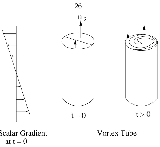
A schematic is shown in Figure 2.4 of the winding of the axial velocity into a spiral. Scalar variations in the axial direction are distorted by the spiraling axial velocity, and we can capture this effect with the following analysis. We begin by defining the material derivativeD/Dt=∂/∂t+ui∂/∂xi and temporarily setν =D = 0. Then we

can rewrite equation (2.47) for c₃ asDc₃/Dt= 0, and it is clear that c₃ is conserved along paths χi(t) that satisfy dχi/dt = ui. Therefore, using the initial condition

(2.51) we have thatc₃(x, t) =µ χ₃(0) whereχi(t) =xi. We can also rewrite equation

(2.46) as Dv₃/Dt = −a v₃, so that v₃(X, t) = exp(−a t)v₃₀ where v₃₀ is a constant, and

dχ₃(t)

dt =a χ3(t) +e −a t_v

(38)

Scalar Gradient

at t = 0

t = 0

Vortex Tube

u

t > 0

3

Figure 2.4: Schematic representation of the winding of the axial velocity in a vortex structure. Scalar variations in the axial direction are in turn distorted by the axial velocity.

This equation can be solved to give

χ₃(0) =χ₃(t)e−a t−v₃(x₁, x₂, t)1

a sinh(at), (2.53)

so that

c₃(x, t) = µ(e−a tx₃ −v₃(x₁, x₂, t)1

asinh(a t)). (2.54)

It is easily verified by direct substitution that this solution (2.54) forc₃ is also valid in the case when ν 6= 0 if Sc = ν/D = 1. To simplify the analysis, we subsequently assume Sc= 1.

Solutions for c1, c2 and the axial velocity and vorticity

Bothc₁ andc₂ have nox₃ dependence initially, and so from equation (2.47) it is clear that they will be independent of x₃ at later times. We are thus motivated to study solutions to equation (2.47) when there is no x₃ dependence,

∂c₁ ∂t +

µ

a₁x₁+∂ψ3

∂x₂

¶

∂c₁ ∂x₁ +

µ

a₂x₂− ∂ψ3 ∂x₁

¶

∂c₁

∂x₂ =D∇

2_c

(39)

It is convenient to work in polar coordinates (r, θ) withx₁ =rcosθ,x₂ =rsinθ, and introduce the transformation [29],

S(t) = ea t, (2.56)

ρ = S(t)1/2r, τ = 1

a(S(t)−1), ψ₃(r, θ, t) = Ψ₃(ρ, θ, τ), ω₃(r, θ, t) = S(t)W(ρ, θ, τ),

v₃(r, θ, t) = S(t)−1U(ρ, θ, τ), c₁(r, θ, t) = Φ(ρ, θ, τ).

Equations (2.46) and (2.55) can then be expressed in essentially the same form,

∂U ∂t +

1

ρ

µ

∂Ψ₃

∂θ ∂U

∂ρ − ∂Ψ₃

∂ρ ∂U

∂θ

¶

=ν∇2₂U, (2.57)

where the equation is also valid if (U, ν) are replaced with (Φ, D). Approximate solutions for W, Ψ₃, U and Φ can be found using a two time analysis [40]. These solutions are asymptotically correct for large τ. The solution for the axial vorticity and the stream function takes the form

W =

∞

X

−∞

ωn(ρ, τ) exp(i n θ), ω−n=ω∗n, (2.58)

Ψ₃ =

∞

X

−∞

ψn(ρ, τ) exp(i n θ), ψ−n=ψn∗, (2.59)

where the Fourier coefficients forn 6= 0 are

ωn(ρ, τ) =fn(ρ) exp(−i nΩ(ρ)τ −ν n2Λ2τ3/3), (2.60)

(40)

with

hn(ρ) =

fn(ρ)

n2Λ2, Λ(ρ) =

dΩ(ρ)

dρ . (2.62)

Theθaveraged angular velocity Ω(ρ) is related to the zeroth harmonic of the vorticity and to ψ₀ by

ω₀(ρ) = 1

ρ

∂(ρ2Ω)

∂ρ , Ω(ρ) = −

1

ρ ∂ψ₀

∂ρ . (2.63)

It should be noted that we assume Λ < 0 in order for the expansion in large

τ to be valid. The expressions for ωn are valid to O(1) for n 6= 0. However ω0

(and hence Ω) is constant in time to within terms of orderτ−2. The functions fn(ρ)

may be viewed as initial conditions that define a spiral vortex structure although the solution is of course only valid for large τ. The above solution for the axial vorticity essentially describes the winding of the non-axisymmetric part of the vorticity field by the axisymmetric part (the core). The solution for the stream function may be rewritten in the form

Ψ₃ = Ψ(0)+τ−2Ψ(2),

Ψ(2) =

∞

X

−∞,n6=0

Ψ(2)_n exp(i n(θ−Ωτ)),

Ψ(2)_n = hn(ρ) exp(−ν n2Λ2τ3/3). (2.64)

The asymptotic solutions for the scalar and the axial velocity are then given by (to order τ−1)

Φ(ρ, θ, τ) = Φ(0)+τ−1 ∞

X

−∞,n6=0

Φ(1)_n exp(i n(θ−Ωτ)),

Φ(0) =

∞

X

−∞

Φ(0)_n (ρ, τ) exp(i n(θ−Ωτ)),

Φ(0)_n = Φˇ(0)_n (ρ) exp(−D n2Λ2τ3/3),

Φ(1)_n = i

ρ ∞

X

−∞,m6=0

Ã

mΨ(2)_m ∂Φ (0)

n−m

∂ ρ −(n−m) ∂Ψ(2)m

∂ ρ Φ

(0)

n−m

!

(41)

Scalar Gradient

Vortex Tube

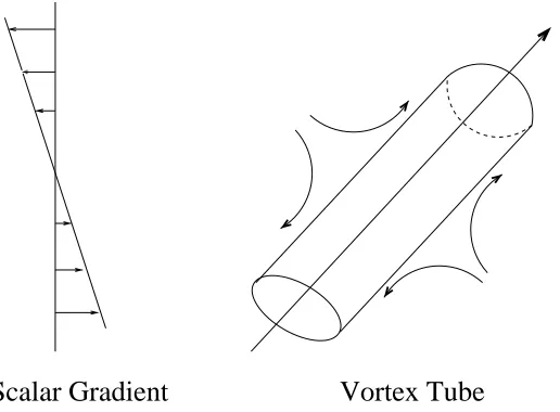
Figure 2.5: Schematic representation of a stretched vortex structure and the mean scalar gradient.

U(ρ, θ, τ) = U(0)+τ−1 ∞

X

−∞,n6=0

U(1)

n exp(i n(θ−Ωτ)),

U(0) ₌ X∞

−∞

U(0)

n (ρ, τ) exp(i n(θ−Ωτ)),

U(0)

n = Uˇn(0)(ρ) exp(−ν n2Λ2τ3/3),

U(1)

n =

i ρ

∞

X

−∞,m6=0

Ã

mΨ(2)_m ∂U (0)

n₋m

∂ ρ −(n−m) ∂Ψ(2)m

∂ ρ U

(0)

n−m

!

, (2.66)

where the initial scalar field is given by the functions ˇCn(0)(ρ) and the initial axial

velocity field is given by the functions ˇUn(0)(ρ). It should be emphasized that this

scalar solution is only valid when the initial conditions have no x₃ dependence, as is the case for c₁ and c₂.

2.2.2

Calculation of the cospectrum

(42)

We will first consider the shell-summed cospectrum defined by equation (2.2). Here we will again adopt the temporary notation where xi are vortex fixed axes,

primed quantities indicate the lab frame, and of coursek =k0, so that equation (2.2) is rewritten as

Cu0_ic(k) =

1 (2π)3

Z

S

Z

V

Ru0_ic(r0)e−ik

0_·_r0

dr0dSk0. (2.67)

We suppose there is a box populated by a collection of stretched vortex tubes. The vortex tubes do not interact except in that each vortex tube is stretched on average by the other vortex tubes. We assume that the vortex structures are distributed sparsely enough so that the overlapping velocity and scalar fields from the vortex tubes do not contribute strongly to the fine scales. It is further assumed that a statistical equilibrium has been reached whereby the structures are created and decay at the same rate. The average in the definition of the scalar-velocity correlation (2.1) is then interpreted as an average over time, space, vortex orientation, and initial conditions of one vortex tube,

Ru0_ic(r0) = Nch<

Z tc

0

Z

V

u0_i(x0, t)c(x0 +r0, t)dx0dt >i, (2.68)

where Nc _{is the rate of creation of vortex tubes per unit time and per unit volume,}

tc is a typical vortex lifetime, hiindicates an average over initial conditions, and <>

indicates an average over vortex orientation. The average over vortex orientation is defined using the Euler angles α, β, γ that rotate the lab frame to the vortex fixed frame [42],

< f(Mij)>=

1 8π2

Z ₂π

0

Z ₂π

0

Z π

0

f(Mij)P(α, β, γ) sinα dα dβ dγ, (2.69)

whereP(α, β, γ) is the probability density function of the Euler angles, andMij is the

associated rotation matrix. To match with experiment we specialize to the case of an isotropic velocity field and set P = 1 so that all orientations are equally likely. We now rewrite equation (2.67) by changing the ordering of the averages, substituting

(43)

x0 to x. It is also convenient to replace the scalar fluctuation, c(x, t), with the total scalar field, ct(x, t), and this is justified because the average of the velocity field is zero. Lastly, we substitute vj(x, t) for uj(x, t), neglecting any contribution from the

strain field. The resulting expression is

Cu0_ic(k) =

Nc

(2π)3 < h

Z

S

Z

V

Z tc

0

Z

V

Mjivj(x, t)ct(x+r, t)e−ik·rdxdt drdSki > .

(2.70)

Simplification using symmetries in the distribution of initial conditions

Next we use some symmetries in the distribution of the initial conditions of the velocity and the scalar to simplify (2.70). For a given vortex tube let the initial v₃

distribution be v₃₀ (say at the time when the tube is created). We will consider the effects of the transformation v₃₀ to −v₃₀. Clearly v₃(x, t) changes to −v₃(x, t) because equation (2.46) is linear and homogeneous. It is also clear that v₁ and v₂

are unaffected as they have no x₃ dependence. From (2.51) we see that initially

∂c₁/∂x₃ = ∂c₂/∂x₃ = 0. Then by taking the partial derivative with respect to x₃

of equation (2.47) we see that ∂c₁/∂x₃ =∂c₂/∂x₃ = 0 for all times. It is then clear from equation (2.47) that v₃ has no influence on the evolution of c₁ or c₂. Finally, it is clear that the first term in expression (2.54) forc₃ is unaffected by changes inv₃₀, and that the second term will change sign when v₃₀ changes sign.

Therefore, if we assume that for each initial distribution of velocities v₁(x,0) and

v₂(x,0) thatv₃(x,0) =v₃₀ is as likely asv₃(x,0) =−v₃₀, then performing the average over the initial conditions will eliminate some terms that we now neglect. At this stage we also neglect the remainder term c0 in the expression (2.50) for ct_(x_{, t}_{). This}