Volume 2010, Article ID 704350,11pages doi:10.1155/2010/704350
Research Article
Time-Varying FIR Equalization for MIMO Transmission over
Doubly Selective Channels
Imad Barhumi
1and Marc Moonen (EURASIP Member)
21College of Engineering, United Arab Emirates University (UAE), P.O. Box 17555 Al-Ain, United Arab Emirates 2ESAT/SCD-KULeuven, Kasteelpark Arenberg 10, 3001 Leuven, Belgium
Correspondence should be addressed to Imad Barhumi,[email protected]
Received 2 November 2009; Revised 13 March 2010; Accepted 8 April 2010
Academic Editor: Xiaoli Ma
Copyright © 2010 I. Barhumi and M. Moonen. This is an open access article distributed under the Creative Commons Attribution License, which permits unrestricted use, distribution, and reproduction in any medium, provided the original work is properly cited.
We propose time-varying FIR equalization techniques for spatial multiplexing-based multiple-input multiple-output (MIMO) transmission over doubly selective channels. The doubly selective channel is approximated using the basis expansion model (BEM), and equalized by means of time-varying FIR filters designed according to the BEM. By doing so, the time-varying deconvolution problem is converted into a two-dimensional time-invariant deconvolution problem in the time-invariant coefficients of the channel BEM and the time-invariant coefficients of the equalizer BEM. The timevarying FIR equalizers are derived based on either the matched filtering criterion, or the linear minimum mean-square error (MMSE) or the zero-forcing (ZF) criteria. In addition to the linear equalizers, the decision feedback equalizer (DFE) is proposed. The DFE can be designed according to two different scenarios. In the first scenario, the DFE is based on feeding back previously estimated symbols from one particular antenna at a time. Whereas, in the second scenario, the previously estimated symbols from all transmit antennas are fed back together. The performance of the proposed equalizers in the context of MIMO transmission is analyzed in terms of numerical simulations.
1. Introduction
The wireless communication industry has experienced a rapid growth in recent years, and digital cellular systems are currently designed to provide high data rates at high terminal speeds. High data rates give rise to intersymbol interference (ISI) due to multipath fading. Such ISI channels are described as frequency-selective. On the other hand, due to the user’s mobility and/or receiver carrier frequency offset (CFO) the received signal is subject to frequency shifts. CFO in conjunction with the Doppler shift give rise to time-selectivity characteristics of the mobile wireless channel. Therefore, the mobile wireless communication channel is generally characterized as time- and frequency selective channel or the so-called doubly selective, which in turns causes degradation in the system performance. This motivates the search for efficient and robust equalization techniques to improve on the information transmission reliability.
The data rate provided by the wireless communication system can be increased substantially by using multiple antennas at the transmitter and at the receiver. It is well-known that multiple-input multiple-output (MIMO) systems can provide an increase in the system capacity by a factor linear in the minimum number of the antennas used at either the transmitter or the receiver [1, 2]. In this paper, we address the problem of equalization for spatial multiplexing-based MIMO transmission over doubly selective channels. Linear and nonlinear decision feedback equalizers are proposed based on the minimum mean-square error (MMSE) and the zero-forcing (ZF) criteria.
as proposed in [5]. Extending the polynomial fitting over the whole packet (or using a sliding window approach) to time-varying frequency-selective channels is investigated in [6]. For single-input multiple-output (SIMO) transmission over doubly selective channels, ZF and MMSE time-varying FIR equalization techniques were proposed in [7]. The extension to the DFE equalizer was presented in [8]. In the MIMO context, the authors in [9] propose block linear filters to mitigate intercarrier interference (ICI) for OFDM transmission over time-varying multipath fading channels. A Kalman filter based MMSE interference suppression is proposed in [10] for MIMO transmission over doubly selective channels. In there, a two-stage suppression tech-nique is proposed; one stage is used to mitigate ISI due to channel frequency selectivity, and another stage is used to mitigate ICI due to channel time selectivity. For estimation of MIMO doubly selective channels, an MMSE pilot-aided transmission is proposed in [11] for cyclic prefix (CP) based block transmission scheme. Optimal training design is proposed in [12]. Adaptive estimation of doubly selective channels is proposed in [13]. There in a subblock tracking scheme for the basis expansion model (BEM) coefficients of the doubly selective channel using periodically transmitted training symbols.
In this paper, we propose matched filter (MF), ZF, MMSE, and DFE time-varying FIR equalizers for MIMO transmission over doubly selective channels. Spatial multi-plexing, where independent data streams are assumed on different transmit antennas, is considered for the MIMO transmission. Considering other MIMO transmission tech-niques, for example, space-time block coding (STBC) [14] is out of the scope of this paper. In the above mentioned schemes, perfect channel state information (CSI) is assumed to be known at the receiver. The basis expansion model (BEM) [15, 16] is used to approximate the underlying communication channel, and to model and design the equalizers. In this sense, a large complex 1D time-varying deconvolution problem is turned into a lower complexity 2D deconvolution problem in the BEM coefficients of the channel and the BEM coefficients of the equalizers.
This paper is organized as follows. In Section 2, the system model is introduced. The time-varying FIR linear equalizers are developed in Section 3. The time-varying FIR DFEs are investigated in Section 4. Our findings are confirmed by numerical simulations introduced inSection 5. Finally, conclusions are drawn inSection 6.
Notation. We use upper bold face letters and lower bold face letters to denote matrices and vectors, respectively. Superscripts H,T, and ∗ represent Hermitian, transpose,
and conjugate, respectively. To simplify notations and save space, the double summation over the subscripts i and j
is denoted as i,j, where the ranges of i and j should
be clear from the context. We denote the N ×N identity matrix asIN, theM×Nall-zero matrix as0M×N. Finally,⊗
denotes Kronecker product,⊕denotes the direct sum, and diag{x} denotes the diagonal matrix with vector x on its diagonal.
x(1)[n]
y(1)[n]
x(Nt)[n]
y(Nr)[n] g(1,1)[n;ν]
g(Nr,1)[n;ν] g(1,Nt)[n;ν]
g(Nr,Nt)[n;ν]
v(1)[n]
v(Nr)[n]
. .
. ...
. . .
. . .
+
+
+
+
Figure1: System model.
2. System Model
We consider an MIMO system with Nt transmit antennas
andNr receive antennas. The input data stream is spatially
multiplexed across theNttransmit antennas, and
transmit-ted over the time-varying multipath fading channel at a rate of 1/Tsymbols/s. Assuming thatτmaxis the maximum delay
spread of all channels and the received symbols are sampled at 1/T samples/s, the channel order L is then obtained as
L = τmax/T+ 1. Thelth tap of the time-varying channel
characterizing the link between the tth transmit antenna and the rth receive antenna at time-index nis denoted as
g(r,t)[n;l] forl = 0,. . .,L. The baseband received signal at
therth receive antenna at time-indexnis obtained as
y(r)[n]= Nt
t=1 L
l=0
g(r,t)[n;l]x(t)[n−l] +v(r)[n], (1)
wherex(t)[n] is the QAM symbol transmitted from thetth
antenna at time-index n, and v(r)[n] is the additive noise
at therth receive antenna. The baseband equivalent of the system described by (1) is depicted inFigure 1.
We will use the BEM [15–17] to approximate the doubly selective channel g(r,t)[n;l] for n ∈ {0,. . .,N + L −1}
(L will be the time-varying FIR equalizer order). In this model, the channel is characterized as a time-varying FIR filter, where each tap of the time-varying FIR is expressed as a superposition of time-varying complex exponential basis functions with frequencies on a DFT grid. The lth tap of the approximated time-varying FIR channel between thetth transmit antenna and therth receive antenna at time-index
nis expressed as
h(r,t)[n;l]= Q/2
q=−Q/2
h(r,t)q,l ej2πqn/K, (2)
where Q is the number of time-varying basis functions. Suppose fmax is the maximum frequency offset of all
channels, the number of time-varying basis functions is chosen such that it satisfies Q/(2KT) ≥ fmax, where K is
y(1)[n]
y(Nr)[n]
w(1,1)∗[n]
w(Nt,1)∗[n]
w(1,Nr)∗[n]
w(Nt,Nr)∗[n]
x(1)[n−d]
. . .
x(Nt)[n−d]
. . .
. . .
. . .
+
+
Figure2: Time-varying FIR linear equalization for MIMO trans-mission.
channel BEM (2) into (1) leads to the following: (note that we use different notations for the true channelg[n;l] and the BEM channel h[n;l] to stress the fact that the BEM model is an approximation of the true channel. However, in the subsequent analysis we proceed as if the channel follows exactly the BEM)
y(r)[n]= Nt
t=1
q,l
ej2πqn/Kh(r,t)
q,l x(t)[n−l] +v(r)[n]. (3)
Casting the received symbols into blocks of lengthN+L, the received vector at therth receive antenna is obtained as
y(r)= Nt
t=1
q,l
h(r,t)q,l DqZlx(t)+v(r), (4)
wherey(r)=[y(r)[−L],. . .,y(r)[N−1]]T
,x(t)=[x(t)[−L−
L],. . .,x(t)[N −1]]T
, and v(r) is similarly defined asy(r).
The diagonal matrixDqrepresenting theqth basis function
is defined as Dq = diag{[1,. . .,ej2πq(N+L−1)/K]T}, and the
(N+ L)×(N +L+ L) Toeplitz matrix Zl is defined as
Zl=[0N+L×(L−l),IN+L,0(N+L)×l].
3. Linear Time-Varying FIR Equalization
In this section, linear time-varying FIR equalizers are derived based on matched filtering (MF), MMSE, and ZF criteria. Each of these linear equalizers consists of a bank of Nt
time-varying FIR filters applied to each receive antenna. The outputs are combined as shown inFigure 2to estimate the transmitted symbols of all data streams on all transmit antennas. An estimate of the symbol of the ath transmit antenna at time-indexnsubject to some decision delaydcan be obtained as
x(a)[n−d]= Nr
r=1 L
l=0
w(a,r)∗[n;l]y(r)[n−l], (5)
where w(a,r)[n;l] is the time-varying FIR equalizer
corre-sponding to the ath transmit antenna and the rth receive antenna, andL is the order of all filters. As the channel is approximated using the BEM, the BEM can also be used to model the time-varying FIR equalizers. The time variation
of each tap is then composed of a superposition ofQ+ 1 complex exponential basis functions with frequencies on the same DFT grid as the BEM of the time-varying channel. Therefore, the lth tap of the time-varying FIR equalizer
w(a,r)[n;l] at time-indexnforn∈ {0,. . .,N−1}is modeled
as
w(a,r)[n;l]= Q/2
q=−Q/2
w(a,r)q,le−j2πq
n/K
, (6)
where w(a,r)q,l is the BEM coefficient of the qth basis of
w(a,r)[n;l]. Substituting (6) into (5) an estimate of the
transmitted symbol on theath antenna at time-indexncan be obtained as
x(a)[n−d]= Nr
r=1
q,l
ej2πqn/K
w(a,r)q,l∗y(r)[n−l]. (7)
On a block level formulation (vector-matrix form), (7) can be written as
x(a)= Nr
r=1
q,l
w(a,r)q,l∗DqZly(r), (8)
where the vector of the estimated symbols x(a) =
[x(a)[−d],. . .,x(a)[N−d+ 1]]T
, theN×Ndiagonal matrix
Dq = diag{[1,. . .,ej2πq(N−1)/K]T}, and the N×(N+L)
Toeplitz matrixZl =[0N×(L−l),IN,0N×l]. Substituting (4)
into (8) yields
x(a)= Nr
r=1 Nt
t=1
q,l
q,l
w(a,r)q,l∗h(r,t)q,l DqZlDqZlx(t)
+
Nr
r=1
q,l
w(a,r)q,l∗DqZlv(r).
(9)
The formula (9) can be further simplified using the property
ZlDq=ej2πq(L−l)/KDqZl, which leads to
x(a)=
Nr
r=1 Nt
t=1
q,l
q,l
ej2πq(L−l)/K
w(a,r)q,l∗h(r,t)q,l DpZkx(t)
+
Nr
r=1
q,l
w(a,r)q,l∗DqZlv(r),
(10)
wherep=q+q,k=l+l, and theN×(N+L+L) matrix
Zk=[0N×(L+L−k),IN,0N×k]. We can now define fp,k(a,t)as
fp,k(a,t)= Nr
r=1
q,l
ej2π(p−q)(L−l)/Kw(a,r)∗
q,l h(r,t)p−q,k−l, (11)
which is a 2D function representing a weighted 2D convolu-tion in the time-invariant BEM coefficients of the equalizer and the time-invariant BEM coefficients of the channel. Substituting (11) into (10) yields
x(a)= Nt
t=1
p,k
fp,k(a,t)DpZkx(t)+ Nr
r=1
q,l
Defining f(a,t) = [f(a,t)
−(Q+Q)/2,0,. . ., f−(a,t)(Q+Q)/2,L+L,. . .,
f(Q+Q(a,t))/2,L+L]T and f(a) = [f(a,1)T,. . .,f(a,Nt)T]T, (12) can
finally be written as
x(a)=f(a)T⊗IN
INt⊗A x+
w(a)H⊗IN
INr⊗B v, (13)
wherex = [x(1)T,. . .,x(Nt)T]T,v =[v(1)T,. . .,v(Nr)T]T, and
the matricesAandBare defined as
A= ⎡ ⎢ ⎢ ⎢ ⎢ ⎢ ⎢ ⎢ ⎢ ⎢ ⎣
D−(Q+Q)/2Z0
.. .
D−(Q+Q)/2ZL+L
.. .
D(Q+Q)/2ZL+L
⎤ ⎥ ⎥ ⎥ ⎥ ⎥ ⎥ ⎥ ⎥ ⎥ ⎦
, B= ⎡ ⎢ ⎢ ⎢ ⎢ ⎢ ⎢ ⎢ ⎢ ⎣
D−Q/2Z0
.. .
D−Q/2ZL
.. .
DQ/2ZL
⎤ ⎥ ⎥ ⎥ ⎥ ⎥ ⎥ ⎥ ⎥ ⎦ . (14)
The time-varying FIR equalizer BEM coefficients vector is defined as w(a) = [w(a,1)T,. . .,w(a,Nr)T]T with w(a,r) =
[w(a,r)−Q/2,0,. . .,w−(a,r)Q/2,L,. . .,w(a,r)Q/2,L]T. We can derive a
rela-tionship betweenw(a) and f(a) as follows. First, define the
(L+ 1)×(L+L+ 1) block Toeplitz matrixHq(r,t)as
H(r,t) q = ⎡ ⎢ ⎢ ⎢ ⎣
h(r,t)q,0 . . . h(r,t)q,L 0
. .. ...
0 h(r,t)q,0 . . . h (r,t) q,L ⎤ ⎥ ⎥ ⎥
⎦, (15)
then define the (Q+ 1)(L+ 1)×(Q+Q+ 1)(L+L+ 1) block Toeplitz matrixH(r,t)as
H(r,t) = ⎡ ⎢ ⎢ ⎢ ⎣
Ω−Q/2H−(r,t)Q/2 . . . ΩQ/2HQ/2(r,t)
0 . .. . .. 0
Ω−Q/2H−(r,t)Q/2 . . . ΩQ/2HQ/2(r,t) ⎤ ⎥ ⎥ ⎥ ⎦, (16)
with Ωq = diag{[ej2πqL/K,. . ., 1]T}. Defining H(t) =
[H(1,t)T,. . .,H(Nr,t)T]T andH =[H(1),. . .,H(Nt)], we can
derive from (11) the following relationship in the BEM coefficients of the time-varying FIR channel and the BEM coefficients of the time-varying FIR equalizers as
f(a)T=w(a)HH. (17)
3.1. Matched Filter Equalizer. The matched filter (MF) equal-izer is the optimal linear equalequal-izer (filter) that maximizes the signal-to-noise ratio (SNR) without necessarily canceling ISI. Defining the SNRo to be the ratio of the power of the
MF output due to the desired signal to the power of the MF output due to the noise as
SNRo=
EqHq
E{nHn} =
trEqqH
tr{E{nnH}}, (18)
where qandn are the first and the second terms of (13), respectively. In this definition,qconstitutes the output due to the desired signal, whilenconstitutes the output due to
noise. Before we proceed, let us first introduce the following properties:
traT⊗I N
V=aTsubtr N{V},
traT⊗IN
U(a∗⊗IN)
=aTsubtrN{U}a∗,
(19)
for an arbitraryk×1 vectora, an arbitrarykN×NmatrixV, and an arbitrarykN×kNmatrixU. The operator subtrN{·}
splits the matrix intoN×Nsubmatrices and replaces each submatrix by its trace (let A be a pN ×qN matrix A = A11 ... A1q
.. . ... ...
Ap1 ... Apq
, whereAi jis the (i,j)thN×Nsubmatrix ofA.
Thep×qmatrix subtrN{A}is then defined as subtrN{A} = tr{A11} ... tr{A1q}
..
. ... ...
tr{Ap1} ... tr{Apq}
). Hence, subtrN{·}reduces the row and
the column dimensionality by a factorN. Assuming that the different data streams are independent and possess the same autocorrelation function such that E{x(i)x(j)H} =R
xδ[i−j]
fori,j =1,. . .,Nt, the SNR at the MF equalizer output can
then be written as
SNRo=
w(a)HHI
Nt⊗RA H
Hw(a)
w(a)HR Bw(a)
, (20)
where RA = subtrN{ARxAH}, and RB = subtrN{(INr ⊗ B)Rv(INr ⊗B
H)}, withR
x andRv are the signal and noise
autocorrelation matrices, respectively. For short we define
Q=INt⊗RA.
Without loss of generality, the MF equalizer w(a) can
be forced to satisfy the constraintw(a)HR
Bw(a) = 1, which
can then obtained by solving the following constrained optimization problem
arg max
w(a) w
(a)HHQHHw(a), s.t.w(a)HR
Bw(a)=1. (21)
The problem in (21) is a generalized eigenvalue problem, with the MF equalizer coefficients are obtained as
wMF(a) =eigmaxR−1
B HQHH
, (22)
where eigmax(A) is the eigenvector that corresponds to the maximum eigenvalue of the matrix A. For a white source (Rx = σs2I), and a white additive noise (Rv = σn2I), and a
BEM resolution withK =N, the SNR at the output of the MF equalizer is obtained as
SNRo=
w(a)HHHHw(a)
w(a)Hw(a)
σ2 s
σ2 n
, (23)
and hence the solution reduces now to
w(a)MF=eigmax
HHH. (24)
This is a special case of (22). However, for K = 2N, and provided that the source and the noise are white, the matrices
3.2. MMSE and ZF Equalizers. In the following, we will derive the linear MMSE and ZF equalizers. Starting with the linear MMSE equalizer, it can be determined by solving the following minimization problem:
arg min
w(a) E
x(a)−Z
dx(a) 2
, (25)
where the multiplication with Zd accounts for the system
decision delay. The minimization (25) can be equivalently written as
arg min
w(a) w
(a)HHQHH+R B
w(a)
−2Rw(a)HHr(a)A
+ trZdRxZTd
, (26)
wherer(a)A =subtrN{(INt⊗A)Rx(e
(a)T
t ⊗IN)ZTd}, withe (a) t is
anNt dimensional unity vector with one at theath position
and zeros elsewhere. Solving forw(a)in (26), we obtain
w(a)MMSE=RB+HQHH −1
Hr(a)A (27)
=R−B1H
HHR−1
B H+Q−1 −1
e(a)d , (28)
where e(a)d = e(a)t ⊗ ed, with ed is a (Q+ Q + 1)(L +
L+ 1) dimensional unity vector with one at position (Q+
Q)(L+L+ 1)/2 +d. Note that (28) is obtained from (27) by applying the matrix inversion lemma ((A+BCD)−1 =
A−1−A−1B(DA−1B+C−1)−1
DA−1), and using the fact that
Q−1r(a) A =e(a)d .
The ZF solution can be obtained from the MMSE solution by setting the signal power to infinity. Hence, the ZF solution is obtained as
w(a)ZF=R−1 B H
HHR−1
B H −1
e(a)d . (29)
For the ZF solution to exist, the matrixH has to be of full column rank. A necessary condition forH to be of full column rank is that the inequality Nr(Q+ 1)(L+ 1) ≥
Nt(Q+Q+ 1)(L+L+ 1) is satisfied. For sufficiently largeL,
andQ, this inequality is satisfied when the number of receive antennas is larger than the number of transmit antennas, that is, Nr ≥ Nt + 1. The MMSE equalizer always exists
regardless of the number of receive antennas. However, the performance of the MMSE equalizer is largely improved if the above inequality is satisfied.
Obtaining the linear MMSE and ZF equalizers involves matrix inversion of sizeP×PwithP=Nt(Q+Q+ 1)(L+
L+ 1). Therefore, the computational complexity of these equalizers requiresO(P3) Multiply-Add (MA) operations.
y(1)[n]
y(Nr)[n]
w(a,1)[n;l]
w(a,Nr)[n;l]
x(a)[n−d]
x(a)[n−d]
. . .
Decision device Feed forward
Feedback −
b(a)[n;l]
+
Figure3: Time-varying FIR DFE-I for theath antenna.
4. Decision Feedback Equalization
In this section we extend the results for linear equalization to decision feedback equalization. The DFE consists of two filters, a forward filter and a feedback filter. The feed-forward and feedback filters are again designed to be time-varying FIR filters. The time-time-varying FIR filters in the forward path are identical to the linear equalizers described
in Section 3.2 (see Figure 2). The feedback filters have as
their input the sequence of decisions on previously detected symbols. Given the extra degrees of freedom offered by the MIMO systems, we can devise two different scenarios. In one scenario, only previously estimated symbols from one transmit antenna are fed back to cancel/reduce ISI in the data stream of that particular transmit antenna. This scenario is referred to as DFE-I. In the other scenario, previously estimated symbols from all transmit antennas are fed back together to cancel/reduce ISI in the data stream of one particular transmit antenna. This scenario is referred to as DFE-II.
4.1. DFE-I. The DFE corresponding to this scenario is depicted inFigure 3. The feed-forward filtersw(a,r)[n;l] are
identical to the linear equalizers developed in the previous section. For each data stream only one feedback filter is used to feedback previously detected symbols of that particular data stream. For the ath data stream, the feedback filter
b(a)[n;l] is again designed as a time-varying FIR filter with
orderL. Hence, an estimate of the transmitted symbol at time-indexnsubject to the decision delaydis obtained as
x(a)[n−d]= Nr
r=1 L
l=0
w(a,r)∗[n;l]y(r)[n−l]
− L+Δ
l=Δ
b(a)∗[n;l]x(a)[n−l],
x(a)[n−d]=Qx(a)[n−d],
(30)
where Δ ≥ d+ 1, and Q(·) is the quantizer used by the decision device. Based on the BEM (6), the time-varying FIR feedback filter on the (l)th tap can be written as
b(a)[n;l]= Q/2
q=−Q/2
b(a)q,le−j2πnq
n/K
where Q is the number of time-varying basis functions. Substituting (31) into (30), and assuming past decisions are correct, yields the following:
x(a)[n−d]= Nr
r=1 Q/2
q=−Q/2 L
l=0
w(a,r)q,l∗ej2πq
n/K
y(r)[n−l]
− Q/2
q=−Q/2 L+Δ
l=Δ
b(a)q,l∗ej2πnq
n/K
x(a)[n−l].
(32)
With a block level formulation, (32) can be written as
x(a)= Nr
r=1 Q/2
q=−Q/2 L
l=0
wq(a,r),l∗DqZly(r)
− Q/2
q=−Q/2 L+Δ
l=Δ
b(a)q,l∗DqZlx(a).
(33)
The first part of (33) is similar to (12), and hence can be written as
x(a)= Nt
t=1
p,k
fp,k(a,t)DpZkx(t)+ Nr
r=1
q,l
wq(a,r),l∗DqZlv(r)
− Q/2
q=−Q/2 L+Δ
l=Δ
b(a)q,l∗DqZlx(a).
(34)
Assuming the feedback filter is designed such thatQ≤Q+
Q, andL+Δ≤L+L, then (34) can be written as
x(a)= Nt
t=1
p,k
fp,k(a,t)DpZkx(t)+ Nr
r=1
q,l
wq(a,r),l∗DqZlv(r)
− p,k
b(a)p,k∗DpZkx(a),
(35)
where b(a)p,k = b(a)q,lδ[p−q]δ[k−l], that is, zeros are
appended in the feedback filter BEM coefficients such that the span of the BEM coefficients of the feedback filter matches that of the sequence fp,k(a). Hence, (35) can finally be
written in a compact vector-matrix form as
x(a)=f(a)T⊗I N
INt⊗A x
+w(a)H⊗IN
INr⊗B −
b(a)H⊗IN
Ax(a).
(36)
Definingb(a) =[b(a)
−Q/2,0,. . .,b−(a)Q/2,L,. . .,b(a)Q/2,L]T, then
b(a)is obtained asb(a)=Pb(a), wherePis a (Q+Q+ 1)(L+
L+ 1)×(Q+ 1)(L+ 1) selection matrix defined as
P= ⎡ ⎢ ⎣
0(Q+Q−Q)/2(L+L+1)×(Q+1)(L+1)
I(Q+1)⊗J
0(Q+Q−Q)/2(L+L+1)×(Q+1)(L+1)
⎤ ⎥
⎦, (37)
with the (L+L+ 1)×(L+ 1) matrixJdefined as
J= ⎡ ⎢ ⎣
0Δ×(L+1)
IL+1
0(L+L−L−Δ)×(L+1)
⎤ ⎥
⎦, (38)
whereΔis restricted toΔ=d+ 1 to simplify the forthcoming analysis. Assuming past decisions are correct, the MMSE-DFE is then obtained by minimizing the error across the decision device as
arg min
w(a),b(a)
x(a)−Z
dx(a) 2
. (39)
Using (34), the mean square-error (MSE) function MSE = x(a)−Z
dx(a)2can be written as
MSE=w(a)HHQHH+R B
w(a)
−2Rw(a)HH(ea⊗RA)
b(a)+r(a)A
+b(a)+ed H
RA
b(a)+ed
.
(40)
Solving for the feed-forward coefficientsw(a) in (40) such
that∂MSE/∂w(a)=0, we obtain
w(a)=R−B1H
Q−1+HHR−B1H −1
I(a)Δ
b(a)+ed
, (41)
whereI(a)Δ =e(a)t ⊗I(Q+Q+1)(L+L+1). Note that, for no feedback
the feed-forward filter in (41) reduces to the MMSE filter solution (28). Substituting (41) into (40), yields the following MSE:
MSE=b(a)+ed H
R(a)⊥
b(a)+ed
, (42)
whereR(a)⊥ is given as
R(a)⊥ =RA−I(a)TΔ
Q−1+HHR−1 B H
−1 HHR−1
B HQI(a)Δ .
(43)
The feedback BEM coefficients are then obtained by solving the following equation:
arg min
b(a) MSE. (44)
To solve for the feedback filter BEM coefficients, we define
u(a) = [b(a)T
−Q/2,. . .,b (a)T
−1 , 1,b
(a)T 0 ,. . .,b
(a)T
Q/2]T, with b (a) q =
[b(a)q,0,. . .,b(a)q,L]T. Hence, (44) is equivalent to the following
constrained quadratic minimization problem
arg min
u(a) u (a)HR(a)
y(1)[n]
y(Nr)[n]
w(1,1)[n;l]
w(Nt,1)[n;l]
w(1,Nr)[n;l]
w(Nt,Nr)[n;l]
b(1,1)[n;l]
b(Nt,1)[n;l]
b(1,Nt)[n;l]
b(Nt,Nt)[n;l]
x(Nt)[n−d]
x(Nt)[n−d]
x(1)[n−d]
x(1)[n−d]
. . . . . . . . . . . . Decision device
Feed forward Feedback
− + + −
Figure4: Time-varying FIR DFE-II for MIMO transmission.
whereR(a)Δ =PTR(a)
⊥ PwherePis a (Q+Q+ 1)(L+L+ 1)×
((Q+ 1)(L+ 1) + 1) selection matrix defined as
P= ⎡ ⎢ ⎢ ⎢ ⎣
0(Q+Q−Q)/2(L+L+1)×(Q+1)(L+1)+1
IQ/2⊗J ⊕J⊕IQ/2⊗J
0(Q+Q−Q)/2(L+L+1)×(Q+1)(L+1)+1 ⎤ ⎥ ⎥ ⎥
⎦, (46)
withJis defined as
J= ⎡ ⎢ ⎢ ⎢ ⎣
0d×(L+2)
IL+2
0(L+L−L−Δ)×(L+2)
⎤ ⎥ ⎥ ⎥
⎦, (47)
ande0 is a (Q+ 1)(L+ 1) + 1 dimensional unity vector
with one in positionQ(L+ 1)/2 + 1. The feedback filter coefficients are then obtained by solving the constrained quadratic minimization problem (45) as
u(a)= R
(a)−1 Δ e0
eT0R(a)Δ −Te0
. (48)
The computational complexity of the feed-forward filter coefficients requires matrix inversion of size P = Nt(Q+
Q + 1)(L+ L+ 1), and hence the complexity is O(P3).
Computing the feedback filter coefficients requires matrix inversion of size (Q + 1)(L + 1) + 1, which requires complexityO(((Q+ 1)(L+ 1) + 1)3). In most of the cases, the feedback filter order and number of time-varying basis functions are smaller than the feed-forward filter order and number of basis functions, that is, (Q + 1)(L + 1)
(Q+Q+1)(L+L+1). Hence, the computational complexity of the DFE of this scenario is dominated by the computation of the feed-forward filter O(P3), which is exactly the same
computational complexity of the linear MMSE or ZF filters. However, the overall complexity is slightly larger for this DFE than the linear equalizers.
4.2. DFE-II. The DFE corresponding to this scenario is depicted inFigure 4. In this scenario, past estimates of sym-bols on all data streams are made available to cancel/reduce ISI. Thus, for each data stream Nt feedback equalizers are
employed. Denote the feedback filter that feedback past decisions of the tth antenna data stream to cancel ISI on theath antenna data stream asb(a,t)[n;l]. Assuming past
decisions are correct, an estimate of the transmitted symbols at time-index n subject to the decision delay d can be obtained as
x(a)[n−d]= Nr
r=1 Q/2
q=−Q/2 L
l=0
wq(a,r),l∗ej2πq
n/K
y(r)[n−l]
− Nt
t=1 Q/2
q=−Q/2 L+Δ
l=Δ
b(a,t)q,l∗ej2πnq
n/K
x(t)[n−l].
(49)
With a block level formulation, (49) can be written as
x(a)=
Nt
t=1
p,k
fp,k(a,t)DpZkx(t)+ Nr
r=1
q,l
wq(a,r),l∗DqZlv(r)
− Nt
t=1 Q/2
q=−Q/2 L+Δ
l=Δ
b(a,t)q,l∗DqZlx(t).
(50)
Assuming the feedback filters are designed such thatQ ≤
Q+QandL+Δ≤L+L, then we can write (50) as
x(a)= Nt
t=1
p,k
fp,k(a,t)DpZkx(t)+ Nr
r=1
q,l
wq(a,r),l∗DqZlv(r)
− Nt
t=1
p,k
b(a,t)p,k ∗DpZkx(t),
(51)
whereb(a,t)p,k =b (a,t)
q,lδ[p−q]δ[k−l]. In a compact vector
form, (51) can finally be written as
x(a)=f(a)T⊗I N
INt⊗A x+
w(a)H⊗I N
INr⊗B
−b(a)H⊗IN
INt⊗A x,
(52)
where b(a) = [b(a,1)T,. . .,b(a,Nt)T]T, with b(a,t) = Pb(a,t),
andb(a,t) = [b(a,t)
−Q/2,0,. . .,b(a,t)−Q/2,L,. . .,b(a,t)Q/2,L]T. The MSE
across the decision device can then be obtained as
MSE=x(a)−Z dx(a)
2
=w(a)HHQHH+RB
w(a)
−2Rw(a)HHQb(a)+e(a)d
+b(a)+e(a) d
H
Qb(a)+e(a) d
.
Solving for the feed-forward coefficients in (53) such that
∂MSE/∂w(a)=0, we obtain
w(a)=R−1 B H
Q−1+HHR−1 B H
−1
b(a)+e(a) d
. (54)
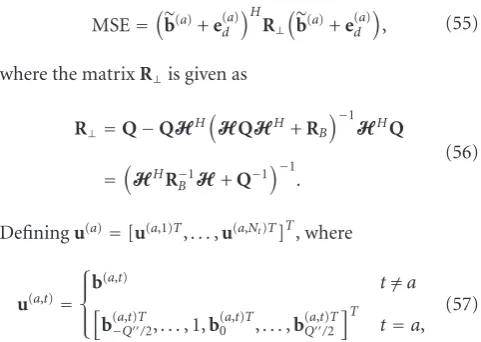
Substituting for the feed-forward coefficients (54) into (53) yields the following MSE
MSE=b(a)+e(a)d HR⊥
b(a)+e(a)d , (55)
where the matrixR⊥is given as
R⊥=Q−QHH
HQHH+R B
−1 HHQ
=HHR−1
B H+Q−1 −1
.
(56)
Definingu(a)=[u(a,1)T,. . .,u(a,Nt)T]T, where
u(a,t)= ⎧ ⎪ ⎨ ⎪ ⎩
b(a,t) t /=a
b(a,t)T−Q/2,. . ., 1,b(a,t)T0 ,. . .,b(a,t)TQ/2
T
t=a, (57)
the MMSE-DFE feedback filter BEM coefficients are obtained by solving for the following constrained quadratic minimization problem:
arg min
u(a) u (a)HR(a)
Δ u(a), s.t.u(a)He (a)
0 =1, (58)
whereR(a)Δ =P(a)TR⊥P(a), with
P(a)=P⊕. . . !"P
ath position ⊕. . .P,
(59)
ande(a)0 is anNt(Q+ 1)(L+1) +1 dimensional unity vector
with one in position (a−1)(Q+1)(L+1)+Q/2(L+1)+1. The feedback filter coefficients are finally obtained as
u(a)= R (a)−1
Δ e
(a) 0
e(a)T0 R(a)Δ −Te(a)0 . (60)
The computational complexity of the feed-forward filter coefficients of this scenario requires matrix inversion of size
P×P, which requiresO(P3) MA operations. This complexity
is the same complexity associated with computing the feed-forward filter coefficients of DFE-I scenario and the linear equalizer. Computing the feedback filter coefficients requires matrix inversion of sizeNt(Q+ 1)(L+ 1) + 1×Nt(Q+
1)(L+1)+1, which requiresO((Nt(Q+1)(L+1)+1)3) MA
operations. In this sense, the computational complexity of DFE-II for the feedback part isNt3times the computational
complexity of DFE-I. Provided that (Q+ 1)(L+ 1)
(Q+Q+ 1)(L+L+ 1), the computational complexity is still dominated by the computation of the feed-forward filter. However, the overall computational complexity for DFE-II is the highest among all devised equalizers.
5. Simulation Results
In this section we present some simulation results for the proposed equalization techniques for MIMO transmission over doubly selective channels. In the simulations, uncoded Quadrature Phase Shift Keying (QPSK) modulation is used. The channel is assumed to be perfectly known at the receiver. The BEM coefficients are then obtained by least-squares (LS) fitting the true underlying channel with the BEM. The performance of the proposed equalization techniques under channel estimation errors is outside the scope of this paper, and a topic of further investigation. The channel taps are simulated as i.i.d random variables, correlated in time according to Jakes’ model with correlation functionrh[n]=
J0(2πn fmaxT), whereJ0is the zeroth-order Bessel function of
the first kind, fmaxT is the maximum normalized Doppler
spread. Two channel setups are used. One with orderL=3, andfmaxT=0.001, and another setup with orderL=6, and
normalized maximum Doppler spread fmaxT = 5×10⁻⁴.
A BEM window size N = 800 is considered all over the simulations. The BEM resolution is chosen such thatK=N
andK = 2N. We measure the performance in terms of bit error rate (BER) versus signal-to-noise ratio (SNR). The SNR is defined as (L+ 1)Es/σn2, whereEsis the transmitted symbol
energy, andσ2
nis the additive white Gaussian noise variance.
In all the simulations the decision delay is taken as d =
(L+L)/2+1, and the approximationRA≈σx2I(Q+Q+1)(L+L+1),
andRB≈σn2I(Q+1)(L+1)are used. It is worth mentioning here
that the BEM approximated channel is used for the equalizers design, but the true channel is used for BER simulations, which will be subject to channel modeling error.
5.1. Channel Setup-I. In this setup the number of basis functions isQ=2 forK =N, andQ=4 forK =2N. Two MIMO setups are considered; a first setup withNt×Nr =
2×4, and a second setup withNt×Nr =2×2. In the first
setup, a linear ZF equalizer may exist, and therefore it can be evaluated against the linear MMSE equalizer and DFE. In the second setup, only the linear MMSE equalizer and the DFE are evaluated.
There are many parameters to tune in the simulations, and to choose the optimal parameter set is a difficult task. In this sense we divided the problem into two sets. In the first set we fixed L andQ and varyLandQat a fixed SNR value. In the second we obtained the optimal (best)L
andQ and varied the feedback parametersLandQ. In this sense, the BER performance is evaluated as a function of the feed-forward filter order L and number of time-varying basis functionsQ at a fixed SNR = 8 dB. The the feedback filters parameters are set atQ = 4, andL = 3, which are the same as the channel BEM parameters. The simulation results corresponding to this setup are shown in
Figure 5. ForK = N the BER is significantly improved for
10−4 10−3 10−2 10−1
BER
3 4 5 6 7
L
8 9 10 11 12
K=N
K=2N
MMSE DFE-I DFE-II
Q=4
Q=8
Q=10 Figure5: BER versusQandLforN
t×Nr=2×4, SNR=8 dB.
10−4 10−3
BER
0 1 2 3 4
L
5 6 7 8
Q=0
Q=2
Q=4
Q=6
Q=8 DFE-I DFE-II Figure6: BER versusQandLforN
t×Nr=2×4, SNR=8 dB.
difference in BER performance for Q = 8 compared to
Q = 10. Taking complexity into account, Q is set at
Q = 8. Setting L = 8, and Q = 8, we also vary the feedback filter parameters Q, and L for the DFE-I and DFE-II scenarios. At an SNR =8 dB, the simulation results are shown in Figure 6. The BER performance improves by increasing Q. For DFE-I scenario the BER performance significantly improves by increasingQup toQ = 4, for which the performance is rather steady. For DFE-II scenario, similar results are observed, except that the performance is slightly best for Q = 6. With regard to feedback filters orderL, the BER performance is significantly improved for 3 ≤ L ≤ 5. Therefore, the feedback filter order is set at
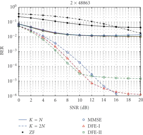
10−6 10−5 10−4 10−3 10−2 10−1 100
BER
0 2 4 6 8
SNR (dB)
10 12 14 16 18 20 2×48863
K=N K=2N
ZF
MMSE DFE-I DFE-II
Figure7: BER versus SNR forNt×Nr=2×4.
L = 3, and the number of time-varying basis functions is set atQ = 6. These specifications of the feed-forward filters are sufficient for the linear ZF equalizer to exist. The simulation results for the BER versus SNR corresponding to this MIMO setup are shown in Figure 7. For K = N, the equalizers suffer from an early error floor at BER = 10−2
except for the linear ZF equalizer which shows a higher error floor at BER = 4×10⁻². For K = 2N, the BER curves
for DFE-I and DFE-II show an error floor at BER = 1.3×
10−6 and BER = 1.5×10⁻⁵, respectively. Benchmarking
at BER = 10−4, DFE-I, and DFE-II outperform the linear
MMSE and ZF equalizers. An SNR gain of 1.3 dB and 2 dB is observed for DFE-I and DFE-II over the linear MMSE equalizer, respectively. The performance of the linear ZF equalizer is very marginal. The performance of DFE-II suffers from a higher error floor than DFE-I, this actually due to the fact that DFE-II is more prone to error propagation than DFE-I, which is clear from the BER figures at high SNR values, where error propagation would become the limiting factor rather than the noise power. This can also be explained based on the structure of each equalizer. Based on their structure, DFE-I feeds back past decisions on only one data stream to cancel/reduce ISI on that particular data stream, while DFE-II feeds back past decisions on all data streams. As such, for DFE-I, incorrect past decisions on one data stream will influence subsequent decisions on only that data stream, while incorrect decisions on one or more data streams for DFE-II will influence subsequent decisions on the other data streams, and hence more likely to propagate. Therefore, DFE-II based on its structure is more vulnerable to error propagation than DFE-I.
For the second setup, the simulation results are shown in
Figure 8. The feed-forward filters are designed to have order
L = 12, and the number of time-varying basis functions
10−4 10−3 10−2 10−1 100
BER
0 2 4 6 8
SNR (dB)
10 12 14 16 18 20 2×2121266
K=N K=2N
MMSE
DFE-I DFE-II
Figure8: BER versus SNR forNt×Nr=2×2.
time-varying basis functionsQ= 6. ForK =N, the BER curves of all equalizers suffer from an early error floor at a BER around BER=3×10⁻². DFE-II marginally outperforms
the linear MMSE equalizer and DFE-I. For K = 2N and benchmarking at BER = 5×10⁻³, an SNR gain of 4 dB
and 5.8 dB are observed for DFE-I and DFE-II, respectively, compared to the linear MMSE equalizer.
5.2. Channel Setup-II. In this setup the number of basis functions isQ = 2 forK = 2N andQ = 4 forK = 3N. An MIMO setup withNt×Nr = 2×4 is considered. The
Linear MMSE and ZF equalizers as well as the nonlinear DFEs are evaluated. The feed-forward filters are designed such that L = 12, and Q = 6. The feedback filters are designed such that L = 6 and Q = 4. The simulation results corresponding to this set up are shown inFigure 9. ForK = 2N, the BER curves for DFE-I and DFE-II show an error floor at BER = 9.2×10⁻⁶ and BER = 5.7 ×
10−5, respectively. Benchmarking at BER=10−4, DFE-I and
DFE-II outperform the linear MMSE and ZF equalizers. An SNR gain of 1.3 dB and 2 dB are observed for DFE-I and DFE-II over the linear MMSE equalizer, respectively. The performance of the linear ZF equalizer is very marginal. For
K = 3N, the different equalizers (the ZF does not exist for this case) exhibit almost the same performance as the
K =2Ncase. A slight performance degradation is observed for the linear MMSE equalizer, this is due to the fact that for this case more parameters to equalize than theK=2Ncase. The DFE equalizers exhibit lower error floor. An error floor of BER=6×10⁻⁶is observed for DFE-I and error floor at
BER=10−5for DFE-II. Again the BER floor of DFE-II is still
higher than the error floor of DFE-I, which again confirms the fact that DFE-II is more vulnerable to error propagation than DFE-I even though with the modeling error is smaller due to the higher BEM resolution.
10−6 10−5 10−4 10−3 10−2 10−1 100
BER
0 2 4 6 8
SNR (dB)
10 12 14 16 18 20 2×461246
K=2N K=3N
ZF
MMSE DFE-I DFE-II
Figure9: BER versus SNR forNt×Nr=2×4 channel setup-II.
6. Conclusions
In this paper, time-varying FIR equalization techniques have been proposed for spatial multiplexing-based MIMO trans-mission over doubly selective channels. The time-varying FIR equalizers are designed considering the matched filter, MMSE and ZF criterion for linear and nonlinear decision feedback equalizers. The BEM is used to approximate the doubly selective channel, and to model and design the time-varying FIR feed-forward and feedback filters. By doing so, the one-dimensional time-varying deconvolution problem is reduced to a two-dimensional time-invariant deconvolution problem in the time-invariant coefficients of the channel BEM coefficients, and the time-invariant coefficients of the BEM equalizers. Using the BEM, and for a sufficient number of BEM parameters, the ZF solution exists forNr ≥Nt+ 1,
which extends a well-known result for the time-invariant MIMO equalization of frequency-selective channels. Using the extra degrees of freedom offered by the MIMO system, a DFE that feeds back the previously estimated symbols on all data streams to cancel/reduce ISI on a particular data stream can be obtained, which is shown to outperform the linear MMSE equalizer and the DFE that feeds back only the previously estimated symbols from one particular data stream. Block equalizers can be derived, but in general require high computational complexity. Hence, time-varying FIR equalization allows for lower complexity equalization techniques.
References
[2] E. Telatar, “Capacity of multi-antenna Gaussian channels,” European Transactions on Telecommunications, vol. 10, no. 6, pp. 585–595, 1999.
[3] L. Lindbom, M. Sternad, and A. Ahl´en, “Tracking of time-varying mobile radio channels—part I: the Wiener LMS algorithm,”IEEE Transactions on Communications, vol. 49, no. 12, pp. 2207–2217, 2001.
[4] E. Eweda, “Comparison of RLS, LMS, and sign algorithms for tracking randomly time-varying channels,”IEEE Transactions on Signal Processing, vol. 42, no. 11, pp. 2937–2944, 1994. [5] D. K. Borah and B. D. Hart, “A robust receiver structure for
time-varying, frequency-flat, Rayleigh fading channels,”IEEE Transactions on Communications, vol. 47, no. 3, pp. 360–364, 1999.
[6] D. K. Borah and B. D. Hart, “Receiver structures for time-varying frequency-selective fading channels,”IEEE Journal on Selected Areas in Communications, vol. 17, no. 11, pp. 1863– 1875, 1999.
[7] I. Barhumi, G. Leus, and M. Moonen, “Time-varying FIR equalization for doubly selective channels,”IEEE Transactions on Wireless Communications, vol. 4, no. 1, pp. 202–214, 2005. [8] I. Barhumi, G. Leus, and M. Moonen, “Time-varying FIR
decision feedback equalization of doubly-selective channels,” in Proceedings of the IEEE Global Telecommunications Con-ference (GLOBECOM ’03), vol. 4, pp. 2263–2268, December 2003.
[9] A. Stamoulis, S. N. Diggavi, and N. Al-Dhahir, “Intercarrier interference in MIMO OFDM,”IEEE Transactions on Signal Processing, vol. 50, no. 10, pp. 2451–2464, 2002.
[10] J. He, G. Gu, and Z. Wu, “MMSE interference suppression in MIMO frequency selective and time-varying fading channels,” IEEE Transactions on Signal Processing, vol. 56, no. 8, pp. 3638– 3651, 2008.
[11] A. P. Kannu and P. Schniter, “Minimum mean-squared error pilot-aided transmission for MIMO doubly selective channels,” in Proceedings of the 40th Annual Conference on Information Sciences and Systems (CISS ’06), pp. 134–139, Princeton, NJ, USA, March 2006.
[12] L. Yang, X. Ma, and G. B. Giannakis, “Optimal training for MIMO fading channels with time- and frequency-selectivity,” inProceedings of the IEEE International Conference on Acous-tics, Speech, and Signal Processing (ICASSP ’04), vol. 3, pp. III821–III824, Quebec, Canada, May 2004.
[13] J. K. Tugnait, S. He, and H. Kim, “Doubly selective channel estimation using exponential basis models and subblock tracking,”IEEE Transactions on Signal Processing, vol. 58, pp. 1275–1289, 2010.
[14] S. M. Alamouti, “A simple transmit diversity technique for wireless communications,”IEEE Journal on Selected Areas in Communications, vol. 16, no. 8, pp. 1451–1458, 1998. [15] G. B. Giannakis and C. Tepedelenlio˘glu, “Basis expansion
models and diversity techniques for blind identification and equalization of time-varying channels,” Proceedings of the IEEE, vol. 86, no. 10, pp. 1969–1986, 1998.
[16] G. Leus, S. Zhou, and G. B. Giannakis, “Orthogonal multiple access over time- and frequency-selective channels,” IEEE Transactions on Information Theory, vol. 49, no. 8, pp. 1942– 1950, 2003.