Volume 2007, Article ID 20248,10pages doi:10.1155/2007/20248
Research Article
Fast
1
Minimization by Iterative Thresholding for
Multidimensional NMR Spectroscopy
Iddo Drori
Department of Statistics, Stanford University, Stanford, CA 94305-4065, USA
Received 18 September 2006; Revised 5 April 2007; Accepted 28 August 2007
Recommended by Sabine Van Huffel
Fast multidimensional NMR is important in chemical shift assignment and for studying structures of large proteins. We present the first method which takes advantage of the sparsity of the wavelet representation of the NMR spectra and reconstructs the spectra from partial random measurements of its free induction decay (FID) by solving the following optimization problem: min
x1subject toy−SFTWTx2≤, whereyis a givenn×1 observation vector,Sa random sampling operator,Fdenotes the Fourier transform, andWan orthogonal 2D wavelet transform. The matrixA=SFTWTis a givenn×pmatrix such thatn < p.
This problem can be solved by general-purpose solvers; however, these can be prohibitively expensive in large-scale applications. In the settings of interest, the underlying solution is sparse with a few nonzeros. We show here that for large practical systems, a good approximation to the sparsest solution is obtained by iterative thresholding algorithms running much more rapidly than general solvers. We demonstrate the applicability of our approach to fast multidimensional NMR spectroscopy. Our main practical result estimates a four-fold reduction in sampling and experiment time without loss of resolution while maintaining sensitivity for a wide range of existing settings. Our results maintain the quality of the peak list of the reconstructed signal which is the key deliverable used in protein structure determination.
Copyright © 2007 Iddo Drori. This is an open access article distributed under the Creative Commons Attribution License, which permits unrestricted use, distribution, and reproduction in any medium, provided the original work is properly cited.
1. INTRODUCTION
High-dimensional NMR spectroscopy is time consuming, requiring between days and weeks of acquisition time [1]. Numerous researchers are interested in reconstructing NMR spectra from undersampled signals [2–5]. For example, strategies include sampling along random lines in the indi-rect dimension and along radial lines. In such methods there are several observations per degree of freedom in the under-lying object. Simple linear methods for reconstruction such as backprojection lead to artifacts when used in an under-sampled setting. More elaborate methods such as maximum entropy suppress artifacts in a nonuniform fashion.
In this work we bring two new elements into play. The first is the idea that there is a rigorously valid sense in which NMR spectra are reconstructed from undersampled data, which includes two components: (i) sparsity: representing spectra in an orthogonal wavelet basis which results in a sparse representation of the signal; and (ii) nonlinear re-construction: application of an optimization criterion which produces a sparse set of representation coefficients. The lim-itation of this approach is computational complexity;
there-fore, the second idea is that for solving these massive opti-mization problems, there are fast iterative algorithms based on thresholding which are used for reconstruction. In this paper, we combine these ideas and demonstrate effective re-construction of 2D NMR spectra using significantly under-sampled data. We experiment with various sampling patterns and perform a detailed comparison of different reconstruc-tion methods.
The wavelet transform is well known and efficiently used for signal compression. It transforms the signal into a do-main in which only a few significant coefficients are required for reconstruction. Considering that a signal to be acquired is sparse under some transform, the idea of this work is to utilize the sparse representation of the NMR signal in some domain to sample in advance only a subset of the signal, thus reconstructing the original signal from a small set of mea-surements.
compressible in a known basis (e.g., wavelet or Fourier) can be reconstructed from fewer measurements than the nomi-nal sampling density, provided that the samples are made on a specially transformed version of the signal. Roughly speak-ing, the samples measure linear functionals which look like random linear combinations of the basis functions and re-construction involves quadratic programming.
In this work, we use the sparsity of the NMR signal inher-ent in the transform domain to sample the signal and recon-struct it. The original signal is recovered by using a nonlinear reconstruction scheme—an approximation to1
minimiza-tion of the transform.
2. 1MINIMIZATION
Formally, the problem we wish to solve is finding the sparsest solution to an underdetermined system of equations:
P0
minx0 subject to y=Ax, (1)
whereyis observed data,Ais a knownn×pmatrix,n < p, andxis an unknown vector inRp. Herex
0represents the
number of nonzeros inxand is not a norm. This is a noncon-vex combinatorial optimization problem. In general, finding the sparsest solution is NP hard [11]. Traditionally, there are three approaches to getting around NP hard problems: if the inputs are very small, an algorithm with exponential time may be satisfactory although not elegant; we may be able to isolate special cases that are feasible in polynomial time; or it may be possible to find a near optimal solution in polyno-mial time using an approximation algorithm. Therefore, we solve the problem for the1norm [12]:
P1
minx1 subject to y=Ax, (2)
which is convex and tractable. In addition, when the solution is sufficiently sparse for certain levels of underdeterminicity there exists equivalence between the1and sparsest solutions
[13].
The notion of using1-penalization as a sparsifying
con-straint has been around for decades. In the context of statisti-cal estimation, this has been made explicit by Efron and Tib-shirani [14,15] who suggested the following1-constrained
minimization:
Lt
min
x y−Ax
2
2 subject tox1≤t. (3)
This problem can also be written in the augmented La-grangian form,
Dλ
min
x
1
2y−Ax
2
2+λx1. (4)
Problems (Lt) and (Dλ) are equivalent. Indeed, it is easy to
verify that forxt∗, a solution of (Lt) for somet ≥ 0, there
exists aλ≥0 such thatx∗t solves (Dλ).
Problem (Dλ) has been introduced to the signal
process-ing community by Chen et al. [12] with the name basis pur-suit denoising (BPDN) [16,17]. This is equivalent to a lin-ear objective perturbed by a quadratic term, yielding thus a
quadratic program, retaining structure similar to linear pro-gramming:
mincTx+1
2p
2
subject to Φx+p=y, x≥0, (5)
wherecTxis the inner product of two vectors withca
vec-tor of ones,Φx is a matrix-vector product such that Φ = (A,−A), andx ≥ 0 means that each entry of the vectorx must be nonnegative.
IfAis orthogonal, theny−Ax2 = y−x2, for y=
ATy, and problem (D
λ) is equivalent to
min
x
1 2
i
yi−xi
2
+λ
i
xi (6)
written coordinate-wise, and therefore we get the soft thresh-olding nonlinearity which solves the scalar minimization problem:
δλ(y)=1
2 arg minx(y−x)
2
+λ|x| (7)
and is the soft thresholding operator:
δλ(y)
i=sgn
yiyi−λ
+. (8)
It is worth noting that (Lt) has been studied by
Tibshi-rani and others in the casen > p, that isAx=yis an overde-termined system of equations, whereas (Dλ) was introduced
[12] and analyzed [18] forn < p.
In most practical settings, we observe noisy data and would like to solve the problem in the presence of noise [16]:
P1,ε
minx1subject to y−Ax ≤ε, (9)
which is equivalent to the optimization problem (Dλ). The
optimization problems (P1) and (P1,ε) can be cast as a
per-turbed linear program which is a quadratic program, and therefore computationally tractable, and solved efficiently using general purpose solvers such as simplex and interior point methods [19,20]. The simplex algorithm moves along the exterior of the feasible region maintaining a solution which is a vertex of the simplex, often solving linear pro-grams quickly in practice, however the algorithm can re-quire exponential time for specific inputs. In contrast, inte-rior point methods move along the inteinte-rior of the feasible re-gion maintaining intermediate solutions which are not nec-essarily vertices of the simplex, and run in polynomial time.
However, for many signal and image processing applica-tions as well as for NMR applicaapplica-tions, the problem sizes are quite large, hence computational complexity is a driving con-cern for these applications. Standard general-purpose solvers such as the simplex and interior point methods can be used; however, general-purpose solvers ultimately require solution of “full” linear systems which may require cubic computation of the orderO(np2) which is prohibitive for large-scale
appli-cations. General-purpose optimizers, while extremely useful for establishing the validity of1-based methods, must give
Recently,1-norm minimization problems have been
ap-plied to a range of important practical applications, particu-larly in conjunction with sparse representation [10,12,17]. The1-norm minimization is a way to attempt to regularize
the solution. Applications have been proposed in the context of time-frequency representation [12], overcomplete signal representation [17], compressed sensing [9,10], MRI [21– 23], removing impulsive noise [24], error-correcting codes [25,26], and genome-wide analysis of mRNA lengths [27].
3. APPLICATION
An important motivation for multidimensional nuclear magnetic resonance (NMR) spectroscopy is to determine the structure of proteins. Briefly, NMR occurs when atomic nu-clei immersed in a magnetic field are exposed to an oscillat-ing magnetic field. When a substance is placed in a magnetic field, some nuclei have orientations called spins. Each spin corresponds to a different energy level and the spins jump between levels when excited by radio waves whose frequency matches the energy spacing, which is called resonance. By changing frequency, the energy level spacings are measured, and a signal is created when the spins flip at resonance. The NMR spectrum shows the magnitude of the signal as a func-tion of frequency.
Numerous processing and analysis steps are performed: beginning with the initial recording of the free induction de-cay (FID), computation of the spectrum, structure interpre-tation and assignment. Several of the key desired properties in this chain of operations are as follows: (i) feasible acqui-sition time for high-dimensional experiments required for handling large proteins, (ii) identifying exact peak positions, and (iii) accurately determining structure from a peak list and additional information. In this work, we focus on the first point which is the most critical bottleneck in practical settings.
Our approach is a general method for fast multidimen-sional NMR by random sampling and fast1 norm
recon-struction by iterative methods. Our main practical result es-timates a four-fold reduction in sampling and experiment time without loss of resolution while maintaining sensitiv-ity for a wide range of existing settings. This is important for chemical shift assignment and for studying protein structure. Recent fast multidimensional NMR methods [28,29] in-clude parallel acquisition schemes, selective recording of out-put spectra, reconstruction from a small set of projections, and reconstruction from random and nonuniform measure-ments.
Replacing serial acquisition in the indirect dimension [30] with parallel acquisition by applying gradients along the
z-axis results in a method for obtaining 2D data in a single scan. This high throughput hardware solution is extended to reconstruction of 3D and 4D spectra by varying gradients of additional axes in encoding. GFT-NMR [1] obtains a full high-dimensional spectrum from a set of low-dimensional spectra by coupling evolution of nuclei thereby reducing the number of indirect dimensions. The approach recovers one d-dimensional spectrum from 2d−k+1k-dimensional spectra,
withd > k, and involves a least squares fit to an
overdeter-mined system of equations. The application of GFT-NMR as demonstrated for the protein ubiquitin results in a reduction of experiment time by an order of magnitude for each re-duced indirect dimension.
Similar to reconstruction methods used in tomography, a full multidimensional spectrum can be reconstructed from a small set of projections [31, 32], utilizing the Fourier projection-slice theorem. More specifically, recent experi-ments include reconstruction of 3D spectra of the small ubiquitin protein and long protein HasA, in which a spec-trum is reconstructed from (t1,t3), (t2,t3) projections as well
as 30, 60 degree projections with respect to thet1axis.
In Hadamard spectroscopy, the evolution periods of the pulse sequences are replaced by arrays which cover a narrow range of the full frequency range. This setting reduces exper-iment time for exploring specific sites. For example, an ex-periment for recovering a subset of peaks in a spectrum of the ubiquitin protein results in a speedup by two orders of magnitude compared with full acquisition.
Multiway decomposition [33] represents the spectrum as a multilinear form consisting of line shapes of peaks. For ex-ample, in the 2D case, the spectrum is represented asXAYT,
whereAis a matrix of amplitudes, andX,Yare shape matri-ces with various constraints such as nonnegativity, symme-try, and orthogonality. This global parametric representation results in filling in a decomposed sparsely sampled signal.
Maximum entropy is often used for reconstruction [2– 5] of a randomly sampled subset of FID measurements in the indirect dimension. As expected, recovery of 3D protein spectra from 20–33 percent sampling of the (t1,t2) plane
re-duces experiment time by factors of 3-4. Both maximum en-tropy and1norm reconstruction use similar sampling
pat-terns; however, our approach is the first to utilize the under-lying sparsity of the NMR spectra in the wavelet domain. An FID has a known mathematical formulation involving a few parameters, however this representation is nonlinear. The representation in the wavelet domain has the advantage of being a linear representation of the signal. The wavelet trans-form has been previously used for smoothing and denoising NMR spectra [30]. In this work, the wavelet transform is im-portant for obtaining a sparse representation of the signal, and the specific transform for a rapid decay of the wavelet coefficients.
4. NUMERICAL SCHEME
In order to reconstruct an NMR spectrum from partial ran-dom measurements of its free induction decay, we solve the following optimization problem:
minx1subject to y−SFTWTx ≤ε, (10)
whereyis the observation,Sis a random sampling operator, F denotes the 2D Fourier transform, andW an orthogonal 2D wavelet transform.
We apply iterative soft thresholding by the iteration
xk+1=xk+δ
tk
A∗y−Axk, (11)
wherexk is thekth approximate solution, δ
t is soft
Input:n×pmatrixA, observation vectory,ε.
Output:solution of (P1,ε).
Algorithm:
Initialization: Residualr0=y. Correlationc0=ATr0. Thresholdt0=max (|c0|). Solutionx0=0 of lengthn. whilerk2≥εy2:
updatesolutionxk+1=xk+δtk(ck). computeresidualrk+1=y−Axk+1.
computecorrelationck+1=ATrk+1.
updatethresholdtk+1=μtk.
end while
Algorithm1: Iterative soft thresholding pseudocode.
increasing iteration count. The “fast operator” composing random sampling, Fourier transform, and the wavelet trans-form is denoted byAand the conjugate byA∗. More specif-ically, we use an orthonormal 2D wavelet transform with 8 vanishing moments.
As mentioned, there exist general purpose solvers for finding the solution of the problem (P1,ε); thus, for
large-scale applications, we introduce efficient special purpose solvers. In addition, recent work [34] has focused on find-ing good sparse approximations for underdetermined linear systems of equations for typical/random matrices; whereas in the next section, we describe in detail fast iterative threshold-ing algorithms suitable for large-scale practical applications.
4.1. Iterative soft thresholding
Iterative soft thresholding, in various guises, has been used for years [30,35,36]. A set of thorough analysis works [37– 41] offer algorithms and proof of their convergence to the global minima of the problems. While not all of these are ex-actly comparable to the our setting, the family resemblance should be clear. In our work, the process of iterative soft thresholding approximately solves (P1,ε) when the solution
is sufficiently sparse andpandnare sufficiently large. A fast solution to the (P1,ε) optimization problem is
ob-tained by a simple iterative soft thresholding (IST) algorithm. Letδt(y) denote the soft thresholding operator:
δt(y)
i=sgn
yiyi−t
+. (12)
Consider the iteration
xk+1=xk+ρδ
tk
ATy−Axk. (13)
Here 0< ρ≤ 1, we start this iteration fromx0 = 0, andt
k
decreases from iteration to iteration. Each iteration requires applications ofAandAT; if these can be performed rapidly,
then each step of IST will run rapidly.
Input:n×pmatrixAand observation vectory,ε.
Output:solution of (P1,ε).
Algorithm:
Initialization: Residualr0=y. Correlationc0=ATr0. Thresholdt0=max (|c0|). Solutionx0=0 of lengthn. whilerk2≥εy2:
computesupportI= {i:|ck| ≥tk−ε}.
solveby least squaresrk=AIdxI.
updatesolutionxk+1=xk+γdx.
computeresidualrk+1=y−Axk+1.
computecorrelationck+1=ATrk+1. updatethresholdtk+1=μtk.
end while
Algorithm2: Iterative thresholding by least squares pseudocode.
We view the sequence of iteratesxkas approximately
fol-lowing the LARS [14] path at thresholdtk. Indeed, this is a
sort of fixed point iteration for the solutionxtwhich satisfies
0=δt(AT(y−Axt)) (14)
which is related to the normal equationsATAx=ATy, and
so, starting from a hypothetical point on the LARS path itself, the iteration would produce no change. Moreover, small per-turbations away from the LARS path produce countervailing adjustments.
Algorithm1describes the pseudocode of the algorithm. In iterative soft thresholding, A andAT are either applied
directly or as fast operators. It is an iterative algorithm in-volving applications ofA andAT which converges rapidly.
A variation on this is a block solution which accelerates the basic soft threshold iteration. The matrix A is partitioned into blocksA = [B1,B2· · ·BJ] by taking random disjoint
columns. Then the least-squares projection ofBj is applied
in computing the correlations:
xk+1,j=xk,j+ρδ
tk
BT
jBj
−1
BT
j
y−Axk. (15)
4.2. Iterative thresholding by least squares
A variant of iterative thresholding, differing in two lines of code, begins with an empty model, an initial estimate of the solution as zeros, and the residual as the observation. We pro-ceed in an iterative fashion, finding the correlations above a threshold and solve a least-squares problem in each iter-ation. This means that in each iteration, as the threshold is decreased, the algorithm solves a least-squares problem us-ing an iterative conjugate-gradient-like method [42] with an increasing number of elements on a larger space. Here,dxIis
4.3. Computational complexity
In this section, we describe the time and space complexity of our algorithms in various settings. In the case whereAis an explicitn×pmatrix such thatn < p, iterative soft thresh-olding described in Algorithm1computes at each iteration kthe residualr = y−Axand correlation vectorsc =ATr,
and applies a soft thresholding operationδt(c). The number
of iterations is typically a small constant depending on the thresholding schedule, and the computational complexity is
O(np).
The iterative method described in Algorithm2computes the residual and correlation vectors as before, and applies a small constant number of conjugate gradient steps to ap-proximately solve the systemATIAIdl(I)= cl(I), withI
de-noting the current active set. Each iteration involves applica-tion ofAIandATI in the order ofO(n2).
We compare this setting to the performance of one spe-cific interior-point method, namely a primal-dual barrier method for convex optimization (PDCO) [19], for solving the linear program arising from (P1). PDCO solves a
stan-dard form linear program by appending a log-barrier term to the objective to replace the nonnegativity constraints and forming the KKT matrix to solve for the Newton update di-rection. The number of iterations is a small constant, and the overall complexity isO(np2). The key point in this case is that
the space complexity which is linear in the input dimension is impractical for large-scale problems such as processing mul-tidimensional signals.
We therefore consider the case whereAis represented as a linear operator which is applied to a vector, for which we coin the term “fast operator”. The Fourier transform, Hadamard transform, and wavelet transform all belong to this class of operators. Such operators are important in large-scale ap-plications, where storing the explicit matrixAis only suit-able for relatively small-scale problems. As described, the main problem with representing the operator as an explicit matrix is that the space complexity isO(np). In large-scale applications it is not feasible to store the matrix in mem-ory. In such a case, when using a “fast operator”, the iter-ative algorithms presented and the specific interior method both have modest space requirements which make them suit-able for large-scale applications. For example, the iterative method only requires storing the current estimate x and residual vector r. Similarly, an efficient implementation of PDCO stores in each stage the current primal and dual so-lution estimates, the next primal and dual steps, and resid-ual. Such space requirements make these methods superior to LARS [14] or OMP [43,44] in large-scale applications. Similarly, the algorithms in1-magic, a collection of
meth-ods for solving convex optimization programs, do not pro-vide a method for solving the problem (Dλ) in which the
matrix is accessed only through matrix-vector multiplica-tions involvingAandATor their fast operators. In this case,
the specific interior-point method discussed above requires computing in each iteration the solution of a system which is prohibitively large, in the order of the data size. When A is given as a fast linear operator, such a system may be solved using a conjugate-gradient-type solver which is
dom-inated by two matrix-vector multiplications per iteration of PDCO.
Implementing the operation of then×pmatrixAas a linear operator may take fewer than n·p operation to ap-ply, and is dependent on the specific operator involved in each application. For example, in the application described in the next section the operator involves random sampling, Fourier transform which is computed by applying the 1-dimensional transform on each dimension in turn in any or-der inO(plogp) independent of dimensiond, and wavelet transform, and therefore time complexity is equal to the time complexity of applying a given operator.
5. SIMULATIONS
In one dimension, a characteristic NMR signal is simulated by a sum of exponentially decaying sinusoids [30] with addi-tive noise as a function of the number of peaks, amplitude, phase, decay time, and frequency:
L
j=1
Ajeiϕj
e−kΔt/τje2πikΔtwj+z. (16)
HereLdenotes the number of sinusoids, each correspond-ing to a scorrespond-ingle nuclear resonance. For each sinusoid j,Aj
denotes the amplitude,ϕj its phase in radians, andτj the
decay time.kdenotes translation,Δtthe sampling rate, and z∼N(0, 1) the additive noise. This results in a spectrum which is the sum of Lorentzian peaks at the frequencieswj.
In our simulation, the amplitude, phase, and frequencies are random uniformly distributed, with constant decay time. A two-dimensional NMR signal is simulated by extending the characteristic one-dimensional equation such that there are separate decays, phases, and frequencies for each dimension d=1, 2. The components in each dimension are of the same amplitude, and the projection onto each dimension is given by
eiϕd,je−td,j
τd,je2πitd,jfd,j. (17)
Two-dimensional NMR was first proposed in 1971 by Jeener and became practical in experiments by Ernst and Freeman. In a normal pulsed NMR experiment, an excitation pulse is followed immediately by data acquisition or detec-tion in which the FID is recorded and data stored. The basic principle of a 2D NMR experiment is that the first variablet1
is the period during which the system evolves, which can be of the order of milliseconds to seconds. This is followed by a constant mixing time which depends on the experiment, in which the spin states are allowed to mix, and finally by a de-tection phase at timet2which is the second variable.
Numer-ous experiments are performed, each with increasing values oft1. When the interferograms (FIDS) from all these
exper-iments undergo Fourier transform with respect tot2we
ob-tain multiple frequency domain spectra f2. If decoupling is
applied during the whole experiment, all of thef2spectra are
20 40 60 80 100 120
20 40 60 80 100 120 (a) OriginalWTx
20 40 60 80 100 120
20 40 60 80 100 120 (b) ReconstructionWTx
0 500 1000 1500 2000 2500 3000
0 20 40 60 80 100 120 140 Original
Reconstruction (c) Slice
Figure1: (a) Original spectrum. (b)1norm reconstruction. (c) Slice of original and reconstructed result.
data acquisition, the nuclei and protons are coupled during the evolution phase. In this work, we perform a realistic sim-ulation of a broad range of 2D NMR spectra by using a data set containing 35 complex signals with varying parameters, including the rate of decay, noise, and peak crowdedness. The data set is used in an experiment management system for biomolecular NMR [45].
5.1. Random sampling
In the application of NMR spectroscopy, random sampling in the indirect dimension of the signal translates into reduc-ing the experiment and actual measurement time. We recon-struct the spectra from the sampled signal by solving an op-timization problem of the form (P1,ε). We set up a system in
which the observation is the signal in scanline order, break-ing up its real and imaginary parts. For example, Figure 1
20 40 60 80 120 100
20 40 60 80 100 120 (a)
20 40 60 80 120 100
20 40 60 80 100 120 (b)
20 40 60 80 120 100
20 40 60 80 100 120 (c)
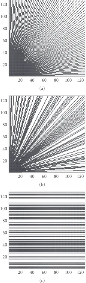
Figure2: Different sampling patterns with a comparable number of samples: (a) equispaced radial lines. (b) Random radial lines. (c) Uniform random horizontal lines.
shows an original spectrum inFigure 1(a), the correspond-ing 1 norm reconstruction from random line samples in
Figure 1(b), and a slice of the original and reconstructed re-sult inFigure 1(c).
Table1: Comparable undersampling factors for different sampling patterns.
Complex points Random lines Radial lines Random radial lines
1282 64 115 114.2
2562 128 133 125.15
5122 256 165 119.6
10242 512 187 129.35
Table2: Dimensions, number of peaks, iterations, reconstruction accuracy, and running times for spectra.
Signal Dimensions Peaks Time (s)
Characteristic 1282 128 42.75
Characteristic 2562 256 146.6
Characteristic 5122 512 427.5
Synthetic 1282 128 45.9
Synthetic 1282 128 46
accuracy. We study the difference between sampling schemes and compare the results empirically.
The mutual coherenceM(A) of a matrixAis the maximal off-diagonal entry of the Gram matrix ATA. Given a
sam-pling pattern as a binary matrixSand a basis matrixB, we form the corresponding Gram matrixG=ATA, whereA=
SB. We compare the quantitiesM(S,B)=maxi=jGi,j/w2
averaged over 100 trials, whereBis the Fourier basis,Sthe various sampling patterns, andw a normalizing scalar. We experiment with different sampling patterns illustrated in Figure 2, while keeping the same undersampling factor as shown inTable 1. As a numerical example, for a given syn-thetic 1282FID with a 2 : 1 sampling ratio, the mean recon-struction error for radial sampling is 0.28 and for random lines 0.67, whereas for a 4 : 1 sampling ratio the mean re-construction error for radial sampling is 0.87 and for ran-dom lines 1.3. This demonstrates improved accuracy in dial sampling compared to random sampling. However, ra-dial sampling commonly results in artifacts. We therefore in-troduce randomness into the sampling to diminish artifacts while maintaining accuracy.
5.2. Reconstruction time
The undersampling factor is important for estimating the re-duction in actual NMR experiment time by simulation using characteristic and synthetic signals. There is a classical trade-offhere, which is that reconstructing the signal requires solv-ing a large optimization problem—our motivation for de-veloping rapid iterative solvers. Therefore the computational efficiency of the nonlinear reconstruction becomes relevant. Reconstruction running times for undersampling by a factor of 2 are summarized inTable 2, on a standard PC running Matlab. The algorithm converges consistently within RMSE of 0.5 in under 50 iterations with a tolerance less than 1e-5 used in the stopping criterion. For a time comparison, solv-ing an instance of the same optimization problem,
ensur-20 40 60 80 120 100
20 40 60 80 100 120 (a)
20 40 60 80 120 100
20 40 60 80 100 120 (b)
0 0.2 0.4 0.8 0.6 1 1.2 1.4
0 20 40 60 80 100 120 140
Number of coefficients
A
ppr
o
ximation
er
ror
(c)
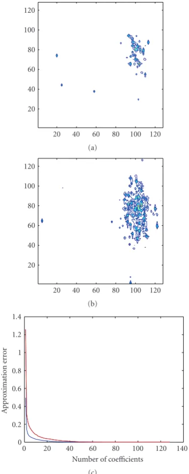
Figure3: (a) Uncrowded and (b) crowded spectra; (c) rapid decay of approximation error for symmlet with 8 vanishing moments.
ing the same tolerance, for a 2562complex FID using PDCO
takes more than three weeks of computation time.
5.3. Analysis of reconstruction results
10−20 10−15 10−10 10−5 100
105
lo
g
re
const
ru
ct
ion
er
ror
18 ×103
0 2 4 6 8 10 12 14 16
Number of coefficients Haar
Beylkin Coiflet 2 Coiflet 4 Daubechies 4
Daubechies 10 Symmlet 8 Daubechies 20 Battle 5
Figure4: Decay of wavelet coefficients of real part on a semilog scale for various wavelets and vanishing moments.
0.4 0.6 0.8 1 1.2 1.4 1.6 1.8
50 100 150 200 250
Number of peaks
Figure5: Mean reconstruction error as a function of the number of peaks for an increasing degree of peak crowdedness.
coefficients of the real part of spectra on a semilog scale for different types of wavelets with varying number of vanishing moments.
The peak crowdedness defines the number of peaks tightly clustered together, and defines the degree of overlap between peaks. We have experimented with reconstruction using a random sampling schedule in the indirect dimension for varying levels of peak crowdedness.Figure 5shows the linear behavior of the mean reconstruction error as a func-tion of the number of peaks for an increasing degree of peak crowdedness.
6. CONCLUSIONS
In conclusion, our methodology provides efficient iterative thresholding algorithms for finding sparse solutions to un-derdetermined systems of linear equations for large-scale practical applications. We demonstrate the applicability of our approach to NMR spectra by utilizing the sparsity of the wavelet transform and provide a valuable tool for speeding-up multidimensional NMR. We would like to compare the accuracy and sensitivity of our approach with maximum entropy reconstruction of high-dimensional spectra [2,3]. Theoretically, it is well known that there exists an equiva-lence between maximum entropy and iterative soft thresh-olding up to a set of parameters. An important contribution of our work compared with maximum entropy spectra re-construction is our use of the wavelet transform to obtain a sparse NMR representation.
ACKNOWLEDGMENTS
The author thanks David Donoho, Yaakov Tsaig, and Jonathan Kaplan for useful discussions. This work was sup-ported in part by grants from NIH Project R01GM072000-03 and NMRA: New Mathematical Methodology for NMR Spectroscopy.
REFERENCES
[1] S. Kim and T. Szyperski, “GFT NMR, a new approach to rapidly obtain precise high-dimensional NMR spectral infor-mation,”Journal of the American Chemical Society, vol. 125, no. 5, pp. 1385–1393, 2003.
[2] M. Mobli, A. S. Stern, and J. C. Hoch, “Spectral reconstruction methods in fast NMR: reduced dimensionality, random sam-pling and maximum entropy,”Journal of Magnetic Resonance, vol. 182, no. 1, pp. 96–105, 2006.
[3] D. Rovnyak, D. P. Frueh, M. Sastry, et al., “Accelerated acqui-sition of high resolution triple-resonance spectra using non-uniform sampling and maximum entropy reconstruction,”
Journal of Magnetic Resonance, vol. 170, no. 1, pp. 15–21, 2004. [4] P. Schmieder, A. S. Stern, G. Wagner, and J. C. Hoch, “Appli-cation of nonlinear sampling schemes to COSY-type spectra,”
Journal of Biomolecular NMR, vol. 3, no. 5, pp. 569–576, 1993. [5] P. Schmieder, A. S. Stern, G. Wagner, and J. C. Hoch, “Im-proved resolution in triple-resonance spectra by nonlinear sampling in the constant-time domain,”Journal of Biomolec-ular NMR, vol. 4, no. 4, pp. 483–490, 1994.
[6] I. Drori, D. Cohen-Or, and H. Yeshurun, “Fragment-based image completion,” ACM Transactions on Graphics (TOG), vol. 22, no. 3, pp. 303–312, 2003.
[7] I. Drori and D. Lischinski, “Fast multiresolution image opera-tions in the wavelet domain,”IEEE Transactions on Visualiza-tion and Computer Graphics, vol. 9, no. 3, pp. 395–411, 2003. [8] A. C. Gilbert, S. Guha, P. Indyk, S. Muthukrishnan, and
M. Strauss, “Near-optimal sparse Fourier representations via sampling,” in Proceedings on 34th Annual ACM Symposium on Theory of Computing, pp. 152–161, Montreal, Quebec, Canada, May 2002.
[10] E. J. Cand`es, J. Romberg, and T. Tao, “Robust uncertainty principles: exact signal reconstruction from highly incom-plete frequency information,”IEEE Transactions on Informa-tion Theory, vol. 52, no. 2, pp. 489–509, 2006.
[11] E. Berlekamp, R. McEliece, and H. van Tilborg, “On the inher-ent intractability of certain coding problems,”IEEE Transac-tions on Information Theory, vol. 24, no. 3, pp. 384–386, 1978. [12] S. S. Chen, D. L. Donoho, and M. A. Saunders, “Atomic de-composition by basis pursuit,”SIAM Journal of Scientific Com-puting, vol. 20, no. 1, pp. 33–61, 1998.
[13] D. L. Donoho, “For most large underdetermined systems of equations, the minimal1-norm near-solution approximates the sparsest near-solution,”Communications on Pure and Ap-plied Mathematics, vol. 59, no. 7, pp. 907–934, 2006.
[14] B. Efron, T. Hastie, I. Johnstone, and R. Tibshirani, “Least an-gle regression,”The Annals of Statistics, vol. 32, no. 2, pp. 407– 499, 2004.
[15] R. Tibshirani, “Regression shrinkage and selection via the lasso,”Journal of the Royal Statistical Society, vol. 58, no. 1, pp. 267–288, 1996.
[16] D. L. Donoho, M. Elad, and V. N. Temlyakov, “Stable recov-ery of sparse overcomplete representations in the presence of noise,”IEEE Transactions on Information Theory, vol. 52, no. 1, pp. 6–18, 2006.
[17] D. L. Donoho and X. Huo, “Uncertainty principles and ideal atomic decomposition,” IEEE Transactions on Information Theory, vol. 47, no. 7, pp. 2845–2862, 2001.
[18] D. L. Donoho and Y. Tsaig, “Fast solution of1-norm min-imization problems when the solution may be sparse,” Tech. Rep. 2006-18, Department of Statistics, Stanford University, Stanford, Calif, USA, 2006.
[19] M. A. Saunders and B. Kim, “PDCO: primal-dual inte-rior method for convex objectives,”http://www.stanford.edu/ group/SOL/software/pdco.html.
[20] Y. Ye,Interior Point Algorithms: Theory and Analysis, John Wi-ley & Sons, New York, NY, USA, 1997.
[21] M. Lustig, D. L. Donoho, and J. M. Pauly, “Rapid MR imag-ing with compressed sensimag-ing and randomly under-sampled 3DFT trajectories,” in Proceedings of the International Soci-ety for Magnetic Resonance in Medicine (ISMRM ’06), Seattle, Wash, USA, May 2006.
[22] M. Lustig, J. M. Santos, D. L. Donoho, and J. M. Pauly, “Rapid MR angiography with randomly under-sampled 3DFT trajec-tories and non-linear reconstruction,” inProceedings of the 9th Annual Scientific Sessions of the Society for Cardiovascular Mag-netic Resonance (SCMR ’06), Miami, Fla, USA, January 2006. [23] M. Lustig, J. M. Santos, J.-H. Lee, D. L. Donoho, and J. M.
Pauly, “Compressed sensing for rapid MR imaging,” in Pro-ceedings of the Signal Processing with Adaptative Sparse Struc-tured Representations (SPARS ’05), Rennes, France, November 2005.
[24] D. L. Donoho and B. F. Logan, “Signal recovery and the large sieve,”SIAM Journal on Applied Mathematics, vol. 52, no. 2, pp. 577–591, 1992.
[25] E. J. Cand`es and T. Tao, “Decoding by linear programming,”
IEEE Transactions on Information Theory, vol. 51, no. 12, pp. 4203–4215, 2005.
[26] M. Rudelson and R. Vershynin, “Geometric approach to error-correcting codes and reconstruction of signals,”International Mathematics Research Notices, vol. 2005, pp. 4019–4041, 2005. [27] I. Drori, V. C. Stodden, and E. H. Hurowitz, “Fast1 mini-mization for genome-wide analysis of mRNA lengths,” in Pro-ceedings of the IEEE International Workshop on Genomic
Sig-nal Processing and Statistics (GENSIPS ’06), pp. 19–20, College Station, Tex, USA, May 2006.
[28] R. Freeman and E. Kupˇce, “New methods for fast multidimen-sional NMR,”Journal of Biomolecular NMR, vol. 27, no. 2, pp. 101–114, 2003.
[29] D. Malmodin and M. Billeter, “High-throughput analysis of protein NMR spectra,”Progress in Nuclear Magnetic Resonance Spectroscopy, vol. 46, no. 2-3, pp. 109–129, 2005.
[30] J. C. Hoch and A. S. Stern,NMR Data Processing, John Wiley & Sons, New York, NY, USA, 1996.
[31] S. Hiller, F. Fiorito, K. W¨uthrich, and G. Wider, “Automated projection spectroscopy (APSY),”Proceedings of the National Academy of Sciences of the United States of America, vol. 102, no. 31, pp. 10876–10881, 2005.
[32] E. Kupˇce and R. Freeman, “Fast reconstruction of four-dimensional NMR spectra from plane projections,”Journal of Biomolecular NMR, vol. 28, no. 4, pp. 391–395, 2004. [33] V. Y. Orekhov, I. Ibraghimov, and M. Billeter, “Optimizing
res-olution in multidimensional NMR by three-way decomposi-tion,”Journal of Biomolecular NMR, vol. 27, no. 2, pp. 165– 173, 2003.
[34] D. L. Donoho, Y. Tsaig, I. Drori, and J.-L. Starck, “Sparse so-lution of underdetermined linear equations by stagewise or-thogonal matching pursuit,” Tech. Rep. 2006-02, Department of Statistics, Stanford University, Stanford, Calif, USA, 2006. [35] S. Sardy, A. G. Bruce, and P. Tseng, “Block coordinate
relax-ation methods for nonparametric wavelet denoising,”Journal of Computational and Graphical Statistics, vol. 9, no. 2, pp. 361–379, 2000.
[36] S. Sardy, A. G. Bruce, and P. Tseng, “Robust wavelet denois-ing,”IEEE Transactions on Signal Processing, vol. 49, no. 6, pp. 1146–1152, 2001.
[37] I. Daubechies, M. Defrise, and C. De Mol, “An iterative thresh-olding algorithm for linear inverse problems with a sparsity constraint,”Communications on Pure and Applied Mathemat-ics, vol. 57, no. 11, pp. 1413–1457, 2004.
[38] M. Elad, “Why simple shrinkage is still relevant for redun-dant representations?”IEEE Transactions on Information The-ory, vol. 52, no. 12, pp. 5559–5569, 2006.
[39] M. Elad, B. Matalon, and M. Zibulevsky, “Coordinate and sub-space optimization methods for linear least squares with non-quadratic regularization,” Journal on Applied and Computa-tional Harmonic Analysis, 2006.
[40] M. A. T. Figueiredo and R. D. Nowak, “An EM algorithm for wavelet-based image restoration,”IEEE Transactions on Image Processing, vol. 12, no. 8, pp. 906–916, 2003.
[41] M. A. T. Figueiredo and R. D. Nowak, “A bound optimization approach to wavelet-based image deconvolution,” in Proceed-ings of the IEEE International Conference on Image Processing (ICIP ’05), vol. 2, pp. 782–785, Genova, Italy, September 2005. [42] C. C. Paige and M. A. Saunders, “LSQR: an algorithm for sparse linear equations and sparse least squares,”ACM Trans-actions on Mathematical Software (TOMS), vol. 8, no. 1, pp. 43–71, 1982.
[43] Y. C. Pati, R. Rezaiifar, and P. S. Krishnaprasad, “Orthogonal matching pursuit: recursive function approximation with ap-plications to wavelet decomposition,” inProceedings of the 27th Asilomar Conference on Signals, Systems & Computers, vol. 1, pp. 40–44, Pacific Grove, Calif, USA, November 1993. [44] J. A. Tropp, “Greed is good: algorithmic results for sparse
[45] P. T. Lee, J. Li, M. R. Chapman, et al., “SESAME: an experiment management system for biomolecular NMR,”
http://www.sesame.wisc.edu.
[46] I. Daubechies,Ten Lectures on Wavelets, CBMS-NSF Regional Conference Series in Applied Mathematics, SIAM, Philadel-phia, Pa, USA, 1994.
Iddo Drori received the B.S. degree in computer science and mathematics in the Amirim program for excellence from the Hebrew University of Jerusalem in 1998 and received the M.S. degree in computer sci-ence with honors from the Hebrew Univer-sity in 2000. He received his Ph.D., in com-puter science from Tel-Aviv University in 2004 and is the receipient of the Maus prize in CS. From 2004 till 2006, he was a