Neural Encoding of Mixtures and Stimulus Generation in the Insect Brain

(1)

Olfactory Object Recognition and

Generalization in the Insect Brain

Thesis by

K

AI

S

HEN

In Partial Fulfillment of the Requirements

for the Degree of

Doctor of Philosophy

California Institute of Technology

Pasadena, California

2010

(2)

Kai Shen

(3)

Acknowledgment

First of all, I would like to thank my graduate advisor, Gilles Laurent for leading me into a fascinating area of research; for both his experimental rigor and clarity of thought; for his appreciation of beautiful data; for his ability to ask the right questions and weave together a great story. I am also very grateful for his understanding during a difficult period in my graduate career, and for allowing me to take a sabbatical to explore other interests, and finally for providing the means for me to travel to Germany to write my thesis. I would also like to thank the other members of my thesis committee: Erik Winfree, for his insights, and valuable suggestions on data analysis; Thanos Siapas, for his skepticism and methodical approach to science that is unsurpassed, and for providing tetrodes for KC recordings that became the foundation to this thesis; and Christof Koch and Michael Dickinson for their valuable support over the years.

(4)

advice, and extraordinary experimental prowess that is inspiring; Glenn Turner, for always being a willing listener, and for his good humor and for his love of science; Cindy Chiu for her encouragement and thoughtfulness; Ben Rubin for all the basketball and life conversations; Vivek Jayaraman for helping me get started in the early days and helpful criticisms; Appreciation also go out to Ofer Mazor, Bede Broome and Mark Stopfer for their advice and expertise in KC recordings; Ueli Rutishauser for discussions about RLSC and science in general; Thomas Nowotney and Ramon Huerta for interesting ideas and different ways of thinking about locust olfaction; and Viola Priesemann for her help in the writing process.

(5)

Abstract

(6)

Contents

Page

ACKNOWLEDGMENTS iii

ABSTRACT

v

TABLE OF CONTENTS vi

1. INTRODUCTION

1

1.1 Object Recognition 1

1.2 Olfactory Computations 5

1.2.1 Nature of odors

1.2.2 Perception of odor mixtures

1.2.3 Odor discrimination

1.2.4 Odor segmentation

1.2.5 Odor generalization

1.3 Olfactory Microcircuits 12

1.3.1 Olfactory receptor neurons

1.3.2 Antennal lobe

1.3.3 Antennal lobe-to-Mushroom body circuit

1.4 Outline and Specific Aims 18

2. MIXTURE CODING AND ODOR-SEGMENTING KENYON

CELLS

20

2.1 Results

22

(7)

2.1.2 Representation of mixtures of increasing

complexity by PNs

2.1.3 Kenyon cell responses to mixtures

2.1.4 PN and KC population statistics

2.1.5 Generating model KC classifiers using recorded PN

data

2.2 Discussion

42

2.2.1 Functional consequences

2.2.2 KCs as independent feature dectors?

2.3 Methods

75

2.3.1 Preparation and stimuli

2.3.2 Binary-mixture experiments

2.3.3 Multi-component-mixture experiments

2.3.4 Electrophysiology

2.3.5 Recording constraints and potential sampling

biases

2.3.6 Extracellular data analysis

2.3.7 Analysis

2.4 Acknowledgements 96

3. ODOR IDENTIFICATION AND GENERALIZATION IN THE

MUSHROOM BODY

97

3.1 Results

98

3.1.1 Decoding PN trajectories over time

(8)

3.2 Discussion

105

3.2.1 Odor segmenting KCs leads to stimulus

generalization

3.2.2 Combinatorial codes for mixtures in the MB

3.3 Methods

126

3.3.1 Mean KC spike latency

3.3.2 Population decoding

4. SUMMARY AND CONCLUSIONS 132

4.1 An elegant solution for odor recognition and generalization

132

4.2 Open questions

134

(9)

C

HAPTER

1

Introduction

Sensory object recognition is the most fundamental of operations

performed by the brain. Computational vision, e.g., has been directed at

understanding how visual objects and their associated properties are

reconstructed and recognized from local information that falls on the

retina (1). In the olfactory system, object recognition involves identifying

characteristic combinations of molecules in complex blends of odorants.

Three fundamental computations olfaction must solve are: recognition,

concentration-invariance, and mixture segmentation.

1.1 Object Recognition

The apparent ease with which we recognize objects belies the magnitude

of this feat: we effortlessly recognize objects from among millions of

possibilities and we do so within a fraction of a second, in spite of

tremendous variation in the appearance of each one (2). Understanding

the computational processes that underlie this ability is one of the

(10)

the ability to accurately discriminate each object from every other object

(‘identification’) or set of similar objects (‘categorization’) from all other

possible objects, and to do this over a range of identity preserving

transformations (e.g., variation in object position, scale, pose and

illumination, and the presence of visual clutter) (2-4). We see an object

many times but never see the exact same image on our retina twice (5).

Although several efforts have examined this so called “invariance

problem” (6-8), a robust, recognition machine still evades us and we lack

a truly satisfying understanding of how the problem is solved by the

brain.

In the visual cortex, evidence suggest that neuronal processes

underlying object recognition are localized in the ventral stream

(V1→V2→V4→posterior IT→anterior IT) (9). The highest stages of this

stream are thought to convey neuronal signals that explicitly support

object recognition – i.e., object identity can be directly extracted from

these populations despite identity-preserving image changes (4, 10, 11).

How are such useful neuronal representations constructed in the brain?

How is it that neurons can be sensitive to subtle changes in object

identity, and yet are relatively insensitive to large identity-preserving

image changes?

Olfaction is very different to vision, because it’s a synthetic sense

(11)

Hopfield (13) postulated several computations that olfactory systems

need to solve that are more sophisticated than simple discrimination.

These include: (i) concentration-invariant odor recognition, (ii)

background-invariant odor recognition, and (iii) odor-mixture

segmentation. Such computations could underlie complex behaviors,

e.g., by tracing a series of sequential odor way-points, salmon can

navigate over thousands of miles from their spawning grounds to the

open ocean and back (14), and rodents have also been shown to track

odors (15). These are examples of computations that have been

proposed but remain poorly characterized at the behavioral level and

unexamined at the neural level.

To recognize an object, an animal must use some internal

representation of the external stimulus (e.g., visual or olfactory scene) to

make a decision: is object A present or not? Computationally, the brain

must apply a decision function to divide an underlying neuronal

representational space into regions where object A is present and regions

where it is not (16, 17). Because brains are essentially networks of

neurons, the subject must also have read-out neurons that can

successfully report if object A was present or not. The central

computational issues of object recognition are (2):

(i) What is the format of the representation used to support the

(12)

i.e., how is the external world represented and what information is

available in the neural code?

(ii) What kinds of decision functions (i.e., read-out tools) are applied to

that representation? i.e., how is the neural code read out by decision

neurons?

Object recognition can thus be viewed as the problem of finding

operations that progressively transform the external world (e.g., visual,

olfactory, auditory stimuli) into a new form of representation, followed by

the application of relatively simple decision functions (e.g., linear

classifiers) that ultimately lead to perception and behavior (2). Along the

way, there are other issues, such as how many neurons are required in

computing the decision function, where are they in the brain, is their

operation fixed or dynamically related to the task (i.e., nonlinearities

involved, learning) and how they code their choices (as a function of

spikes)?

Basic machine learning textbooks tell us that feature selection is

more important than the complexity of the classifier used (SVM, NN or

one of many nonlinear classifiers). It has been shown that a variety of

recognition tasks can be solved in inferotemporal (IT) cortex using simple

linear classifiers (10, 18). The feature vector that results from the

(13)

applied by a decision function due to its high dimensionality and

redundancy. The “curse of dimensionality” tell us that the number of

training examples must grow exponentially with the number of features

in order to learn an accurate model (19). Because only a limited number

of examples are typically available, there is an optimal number of feature

dimensions beyond which the performance of the recognition model

starts to degrade. Thus, dimensionality reduction is crucial in order to

build a classifier with high accuracy. We can think of progressive

transformations from one form of representation to another as extracting

features optimal for decision making, akin to dimensionality reduction.

1.2 Olfactory Computations

1.2.1

Nature of odors

The sense of smell is well known for its ability to detect odorants at levels

far below that of the most sensitive instruments, to discriminate between

thousands of single odorants, and to engrave into memory recollections

of smells that stretch back in time. Our olfactory abilities to detect,

discriminate, and imprint odors is unmatched by any electronic nose.

Naturally occurring odors rarely emanate from a single chemical, it

(14)

sense of smell must have developed, over evolution, to process complex

odor mixtures.

The relationship between odor structure, neural representations

and perception is not deterministic, and depends on experience and

learning (20). Odors are also difficult to quantify because its chemical

structure cannot be described by a simple set of parameters – odor space

is extremely high dimensional and vary in an indeterminate number of

parameters such as carbon-chain length, molecular weight, and polarity.

Recently a multidimensional, physiocochemical odor space was devised to

describe odor structure: 1664 molecular descriptors (thus 1664-d space)

for 1500 odors (21). Each odor was represented as a 1664-d vector in

this space. This odor space maybe useful in predicting odor perception.

Principle component analysis revealed a correlation between odor

structure in this space and its perceived pleasantness among humans

(22).

1.2.2

Perception of odor mixtures

Over the centuries, odor mixtures in the form of fragrances and incense

have been used to suppress or mask a variety of unpleasant odors,

including body odors or those emanating from waste materials, as well as

(15)

most liked and effective fragrance mixtures became known, - e.g.,

jasmine, rose and orange oils are still in use. Our knowledge of brain

mechanisms that computes and recognizes odor mixtures is however

very limited. The study of the perception of odor mixtures by humans

starts with binary mixtures, e.g., (23), and there are several common

outcomes: both odors may be identified with no change in their perceived

intensities compared to their intensities before mixing; both may be

perceived but with one or both having reduced intensity; or one maybe

suppressed to such an extent that it cannot be perceived (24-27). Odor

reduction or suppression is dependent on the particular odor

combination and the concentration of each odor. When binary mixtures

are analyzed by human subjects, discrimination of the individual

components is influenced not only by the type of odor and the perceived

intensity of each component, but also by their familiarity and

pleasantness (28).

In humans, correctly judging whether a binary mixture is different

(discrimination) from a stimulus consisting of only one of the

components is generally much simpler than having to identify one or

both of the components (identification). The ability to identify

components in mixtures becomes increasingly more difficult as the

number of components increase, with the limit at ~4 (25-27).

(16)

was also the most common maximum number of odors chosen in

mixtures containing up to 8 odors. When this experiment was repeated

with mixtures instead of single components, the result was again 4.

Taken together, this indicates that humans encode complex odor

mixtures as single entities.

1.2.3

Odor discrimination

With training, rodents can learn to discriminate between virtually any pair

of pure odors, including highly related stereoisomers (29-31). Rats can

also perform difficult odor discrimination tasks after extensive lesions of

the OB (29), suggesting that simple discrimination (e.g., go/no-go, where

1 bit of information to be extracted) is fundamental to olfactory

processing and not necessarily a computationally difficult task (or at least

not one that requires the entirety of the OB).

1.2.4

Odor segmentation

The 2007 Pixar film Ratatouille is about how a rat Remy, blessed with

unusually sharp olfactory senses, becomes an extraordinary chef. The

food odors in Remy’s kitchen do not exist alone, there are experienced in

the larger context of a variety of different odors and thoroughly mixed.

(17)

ingredients that goes into a soup. Odor segmentation is thus the ability

to identify unique odor objects from a mixture of odors, - an analogy to

the “cocktail party problem” in audition - where a single voice is

recognized from a background of many different noises (32).

Psychophysical experiments in humans show that the limit of identifying

components within mixtures is ~4 (24), but if asked to identify only one

highly familiar odor within mixtures, performance becomes chance only

after 16 odors in the mixture (33). Highly olfactory animals such as rats

likely can do even better (34).

Because odors are thought to be mixed thoroughly at the receptor

level, the computational problem of segmenting particular components is

not necessarily a simple one. By exploiting temporal correlations

between groups of receptors to temporal fluctuations (in concentrations)

of different odor streams, odor mixtures have been decomposed into its

components in a computational model (35). However, the problem

becomes more difficult if the temporal fluctuations are not present, as is

the case when the different components are very well mixed (e.g., aroma

from wine or well cooked meal). Brody and Hopfield (34) implemented a

neural model (termed many-are-equal) using spike-timing computations

allowing for concentration-invariant recognition and odor segmentation

within complex olfactory scenes. Their model relies on differential phase

(18)

apply to the locust antennal lobe (AL, model system of this thesis),

because in our model system, the phase of AL principal neuron firing

contains no information about odor identity or intensity (7).

1.2.5

Odor generalization

Learning strongly influences the ability of animals to perceive and identify

odors. Animals must take information about a conditioned odor

experience and generalize this information to future odor experiences

because no two conditioning stimuli are experienced in exactly the same

way (36). Generalization of a conditioned response, (e.g., a learned

association of an odor with reward), occurs when animals perceive

similarities among stimuli from one experience to the next. Put it more

formally, it is the ability to decide that two odors, though readily

distinguishable, are similar enough to afford the same outcome (36).

One beautiful example in nature is the foraging behavior by honeybees –

they use the odor of flowers to identify a good floral source and forage

on it exclusively (37, 38). Floral scents are intrinsically variable:

substantial variation in the ratios of the compounds exist even for flowers

produced by the same plant (39). A honeybee can learn the odor of a

flower and subsequently compares it to odors emanating from novel

flowers and decides whether or not to forage. It uses several aspects of

(19)

generalize what is learned to novel flowers (39, 40). In a recent study

(41), it was shown that honeybees have the ability to use precise

information about the ratios of two odors in a mixture in order to identify

a rewarding stimulus and to discriminate it from a

punishment-associated stimulus having a different ratio of the same two odors.

Alternatively, if two stimuli differing in odor ratios both lead to a

rewarding outcome, honeybees can learn to ignore information about the

ratio of the two odors and thereafter respond to all mixtures of the same

two odors with equal probability (41).

Fig. 1.1. Locust Olfactory Anatomy. AL, antennal lobe; LH, lateral horn; MB, mushroom

body; OL, optic lobe; agt, antennal-glomerular tract; an, antennal nerve; gl, glomerulus;

on, ocellar nerve; p, pedunculus; βLN, β-lobe neuron; KC, Kenyon cell; LN, local neuron;

ORN, olfactory receptor neuron; PN, projection neuron; d, dorsal; l, lateral; mid, midline.

Adapted from (42, 43).

2

Figure 1.1.Locust Olfactory Anatomy. AL, antennal lobe; LH, lateral horn; MB, mushroom body; OL, optic lobe; agt, antennal-glomerular tract; an, antennal nerve; gl, glomerulus; on, ocellar nerve; p, pedunculus;βLN,β-lobe neuron; KC, Kenyon cell; LN, local neuron; ORN, olfactory receptor neuron; PN, projection neuron; d, dorsal; l, lateral; mid, midline. Adapted from Laurent and Naraghi (1994); MacLeod and Laurent (1996).

cholinergic), as well as local neurons (LNs, GABAergic, but, inDrosophila, some also

cholinergic (Shang et al., 2007)). The neuropil where these synapses are formed is

organized into glomeruli (Figure 1.1A). PNs send axons out of the AL, via the

antennal glomerular tract (AGT), and synapse onto the dendrites of Kenyon cells

(KCs) in the calyx of the mushroom body (MB). Beyond the MB, the bifurcating

axons of PNs also target the Lateral Horn (LH), where they contact inhibitory

neurons (LHIs) (Laurent et al., 2001).

This architecture resembles a simplified version of the mammalian olfactory

bulb (OB): ORNs send axons, via the olfactory nerve (ON), to the OB, where they

contact the principal neurons of the OB, mitral and tufted (M/T, glutamatergic)

cells, as well as periglomerular (PG, GABAergic and/or dopaminergic) cells. The

neuropil where these synapses are formed is organized into glomeruli. M/T cells

(20)

1.3 Olfactory Microcircuits

1.3.1

Olfactory receptor neurons

Olfaction can be thought of as a series of representations and

re-representations of the external olfactory world that ultimately allows the

nervous system to use it for perception and behavior. The primary

representation of an odor is in the response profiles of olfactory receptor

neurons (ORNs, ~1300 ORNs from each antenna project bilaterally to the

AL in Drosophila). The number of unique olfactory receptor (OR) types is

very large in most species (~60-1000), making olfaction fundamentally

different to other sensory modalities (13). Most ORNs express only one

OR (some 2-3), but the same OR is never expressed by more one ORN

type (20). The signaling of specific ORNs thus reflects the activity of

specific odor receptors. From systematic studies of ORN responses to

many odors (44) three basic principles emerge: (i) individual odors

activate subsets of ORNs; (ii) individual ORNs are activated by subsets of

odors with varying breadth of tuning. Broadly tuned receptors are most

sensitive to structurally similar odors; (iii) increasing odor concentrations

elicit activity from greater numbers of ORNs. Thus, both odor identity

and intensity are represented combinatorially across the receptor

population. However, there also exist very specialized channels that are

highly selective to certain chemicals. In moths, there are dedicated to

(21)

ORN type is highly selective for 4-methylphenol which is present in our

sweat (45); CO2 as low as 0.1% also activates a single glomerulus (V

glomerulus) in flies and in turn induces robust avoidance response, CO2

are released by flies under stress (46).

1.3.2

Antennal lobe

In insects, ORNs send axons, via the antennal nerve (AN), to the antennal

lobe (AL), where they contact the principal neurons of the AL, projection

neurons (PNs, cholinergic), as well as local neurons (LNs, GABAergic, but,

in Drosophila, some also cholinergic (47)). The neuropil where these

synapses are formed is organized into glomeruli (Fig. 1.1). In most

insects, ORNs that express the same receptor converge upon one or two

glomeruli (32). The convergence ratio from ORNs is high, ~50 ORNs onto

an average of ~3PNs per glomerulus each ORN contacts all PNs in the

glomerulus) and with reliable synapses in Drosophila (48). This is

thought to increase signal-to-noise ratio in PNs (making one PN more

informative than one ORN). Most individual PNs receive direct excitatory

input from only one type of ORN, expressing one type of odor receptor,

in locusts, each PN receives input from 10-14 glomeruli (out of ~1000)

with ill-defined boundaries; correspondingly, individual ORN axons

project to several glomeruli (32). It is not known whether all ORNs of the

(22)

whether the glomeruli visited by each PN are innervated by ORNs of the

same type. Both PNs and LNs receive direct excitatory synapses from

ORNs. There are also neuromodulatory neurons that release

neuropeptides such as dopamine, octopamine and serotonin, in the AL;

these releases are believed to alter PN responses during associative

learning (49).

PNs form direct excitatory synapses onto LNs, LNs in turn inhibit

PNs, together they form a recurrent network (32). This interplay between

excitation and inhibition gives rise to AL dynamics at two time scales (50,

51). First, PNs respond to odors with slow temporal spike patterns that

outlast the odor stimulus (12). These patterns include both excitatory

and inhibitory epochs. Second, PNs transiently synchronize with each

other during an odor presentation (52). This transient synchrony gives

rise to ~20-30Hz oscillations seen in the local field potential (LFP:

representative of summated synaptic potentials of the PN outputs

measured in the Mushroom body). These odor-evoked oscillations are

also visible in the subthreshold activity of PNs, LNs and the recipients of

PN output in the MB, the Keyon cells (53). GABAA conductances in LNs are

thought to underlie these oscillations, which can be abolished with

(23)

1.3.3

Antennal lobe-to-Mushroom body circuit

PNs send axons out of the AL, via the antennal glomerular tract (AGT),

and synapse onto the dendrites of Kenyon cells (KCs) in the calyx of the

mushroom body (~50,000 KCs in each locust MB). Beyond the MB, the

bifurcating axons of PNs also target the Lateral Horn (LH), where they

contact inhibitory neurons (LHIs) (54). The MB is a bilaterally symmetrical

structure consisting of a calycal neuropil, which forms a cup beneath a

large number of KC somata, and a pedunculus that terminates in two or

more lobes. The KCs send their dendrites into the calyx and their axons

make up the pedunculus and subsequently bifurcate into the lobes. The

input to the calyx is predominantly olfactory, from PNs. The output of

the MB appears to be restricted to the lobes, where KC axons contact MB

extrinsic neurons. The KC population can be divided into multiple types,

as determined by anatomical methods (55). In the pedunculus and lobes,

KC axons appear to segregate into multiple concentric or parallel layers,

subsets of which are selectively invaded by individual MB extrinsic

neurons. The MB has been compared to three different regions in the

mammalian brain (56): first, the hippocampus, because of its involvement

in learning and memory; lesioning the MB in cockroaches impairs their

memory for spatial locations, much like hippocampal lesions do in

rodents (57). Second, the cerebellum because of its involvement in

(24)

compared to the piriform cortex because both are two synapses

downstream of the olfactory sensory layer.

KCs are activated by subsets (50 ± 15%) of coincident PNs, with

high threshold, and integrate over ~1/2 an oscillation cycle (25 ms), are

driven most strongly during the most dynamic epochs of PN firing (58,

59). Furthermore, voltage-gate channels in KC dendrites amplify

responses to coincident PN inputs nonlinearly, further narrowing the

integration time-window (60). These circuit operations between PNs and

KCs results in a marked transformation from broadly tuned cells (PNs) to

highly odor-selective ones (KCs) (53, 61). This sparse, selective property

of KCs has great benefits for memory storage, because if a neuron (i.e.,

PN) responds to multiple odors, synaptic plasticity driven by one odor

could perturb memories formed by a different odor (a problem known as

synaptic interference). Such sparse codes have also been found in many

other systems (11, 62, 63), and more recently, odor coding has also been

found to be sparse in the pyramidal neurons of the piriform cortex (64),

an analogue of the MB in rodents.

In many animals, certain odors elicit innate behavioral responses in

addition to pheromonal responses (20). Both insects and mammals can

be innately attracted to or repelled by certain odors through a mechanism

that depends on the activation of specific glomeruli (20, 65). These

(25)

specific neurons in higher centers – (i) PN axons from the same

glomerulus show stereotyped projections to the LH (66); (ii) PNs

associated with food odors and pheromones target different regions of

the LH (67). In comparison, a recent electrophysiological study did not

find a high level of stereotypy in the MB (68). Experiments that lesion or

inactivate the MB suggest that information flow through the LH alone is

sufficient to support basic olfactory behaviors (69), while the MB is

required for associative olfactory learning. In Drosophila, there are ~ 50

MB extrinsic neurons that decode the MB neuronal output (48), in locusts,

there likely more (Stijn Cassenaer, personal communication). This shows

that after the fan-out (PNs to KCs), there is now again a fan-in (KCs to MB

output) as the system is closer to motor output. These synapses are

likely changed during associative learning (48). It was recently

discovered that there exists a form of spike-timing-dependent plasticity

(STDP) at the synapse between KCs and a class of output neurons, termed

β lobe neurons (βLNs) (70). Synapses that were active a few milliseconds

before these βLNs spiked were strongly potentiated, while those synapses

(26)

1.4 Outline and Specific Aims

How does the brain achieve both fine recognition of particular odor

objects (selectivity) and generalization across categories of odor objects

(invariance)? The focus of this thesis is in answering the computational

aspects of the aforementioned question, using the locust olfactory

system as a model system. The approach I will take is to investigate how

neural representations of odor components and mixtures are transformed

from the projection neurons (PNs) of the Antennal lobe to the Kenyon

cells, intrinsic cells of the Mushroom body, and how KC population data

could be read out. In particular, the emphasis of this work will be on the

analysis of population neural data of both PNs and KCs. A PN-KC model

is implemented and fed with experimental PN inputs that will

demonstrate at a detailed mechanistic level, how KC properties observed

experimentally could be derived.

The work presented in Chapter 2 builds on a large body of previous

research that has elucidated the roles of different elements of the locust

olfactory system and described some of the rules governing their

interactions (7, 42, 43, 53, 58-60, 71, 72). This work has led to a fairly

detailed understanding of the mechanisms that underlie the integration

of ensemble PN input by KCs in the MB. But insofar, no detailed and

systematic examination of multi-component mixtures have been

(27)

experimental study of odor segmentation in any neural system (with

mixtures beyond 3 components). I will examine the following questions:

What are the neural representations of odors and mixtures in the AL and

how are they re-represented again the MB? Can we reproduce the

characteristics of KCs that we observe experimentally from what we know

about the biological constraints of the system.

Chapter 3 applies for the first time a population decoding method

to Kenyon cells. What is crucial are the informational aspects of odor

stimuli (e.g., category vs. identity) that are represented in the KC

population response, because this representation is used by downstream

neurons for associative learning and subsequent behavior output.

Chapter 3 is organized to answer four questions: (i) What types of

olfactory information is extracted by KCs from the PN input? Or put it

another way, what types of information is contained in the KC population

response? (ii) What is the format of this representation? And how is it

different to the format of the PN representation? (iii) What is this format

useful for? (iv) How is the KC population response read out by

downstream neurons? The work in Chapter 2 and 3 is in preparation for

publication as Shen, K., Tootoonia, S. and Laurent, G.

Chapter 4 concludes the thesis and presents some open questions

(28)

C

HAPTER

2

Mixture Coding and

Odor-segmenting Kenyon Cells

The main computational problems of olfaction include odor

discrimination (29-31, 73, 74), concentration-invariant recognition (7,

75, 76), classification (grouping of stimuli by shared features),

generalization (assignment of novel stimuli to a group, based on shared

features), and odor segmentation (of components from within a mixture,

of signal from background) (32, 77). These object recognition problems

(2) are not specific to olfaction but they are interesting to study from

within it, because olfactory systems are structurally shallow and thus

solve them in very few steps. Using locusts as models, we gained some

understanding of the representation formats for simple odors in the first

three relays of its olfactory system—the antennal lobe (AL), mushroom

body (MB) and beta lobe (βL)—and of the computations carried out by

these circuits (7, 53, 58, 70). We also discovered that odors at different

concentrations generate low-dimensional manifolds of spatio-temporal

(29)

invariance. In this study, we turn to odor mixtures. Most natural odors

comprise many components, usually mixed in particular ratios. Mixtures

can be perceived as wholes (“coffee”, “grapefruit”) (33), but they can also

be classified into categories, with various degrees of refinement (“fruity”

→ “citrusy” → “grapefruit”). In addition, humans can identify as many as

8-12 familiar odors in a blend (33), animals such as insects and rodents

can likely do better (78). These observations are interesting, because the

computational constraints on generating a unitary percept and on

segmenting a stimulus into its components are contradictory. Our goal

was thus to discover, using the locust system, whether and how the

formats of representations for odor mixtures might be consistent with

these competing requirements. In the first set of experiments, we

investigated neural representations to two odors and analyzed how these

responses changed when the stimulus was “morphed” from one odor to

another through a series of intermediate mixtures (binary mixture

experiments, see Methods). In the second set of experiments, we chose a

set of eight monomolecular odors, paraffin oil (their dilution substrate)

and mixtures of two, three, four, five and eight of those odors (44 stimuli

in all, out of 211 possible, see Methods). We recorded from 343

projection neurons (PNs, the analog of vertebrate mitral cells, 168 PNs for

binary experiments, 175 PNs for multi-component mixture experiments)

and 209 Kenyon cells (KCs, the mushroom body neurons, for

(30)

2.1 Results

2.1.1

Representations of binary mixtures by PNs

Because odor representations by PNs are highly distributed and varied in

time (Fig. S2.3), because their activity patterns are decoded by individual

KCs on which converge many PNs (59) and because KCs have very short

effective temporal integration windows (53, 60), it is appropriate and

more informative to examine PN responses as time-series of

instantaneous population vectors, or trajectories, in an appropriately

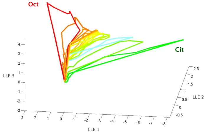
reduced state space (7, 58, 71, 79). Figure 2.1 illustrates these PN

population trajectories for a set of representative stimuli. Figures 2.1A-C

concern binary mixtures: we plot the evolution of the representation for

the odors citral, octanol, and their 1:1 mixture. The mixture trajectory

lies somewhere in between those for the two components, suggesting a

simple linear combination. This was confirmed by correlation analysis

performed in full PN space. This relatively simple combination was not

entirely predictable from the responses of single PNs to binary mixtures,

for those often deviated significantly from the arithmetic sum of the

responses to the components (Fig. S2.3; compare open and filled PSTHs).

This suggests that significant correlations exist between the responses of

different PNs to the same stimulus, and that those linearize the

population's combined output, at least for binary mixtures. Figure 2.1B

(31)

odors and their binary mixture). Extending previous results (7), we find

that concentration series for 1:1 mixtures, as for single odors, generate

families of closely related trajectories (lower-dimensional manifolds),

clustered by odor rather than concentration. In a final experiment, we

“morphed” one odor into the other in 11 intermediate steps (Fig 2.1C).

Contrary to recent results in the zebrafish olfactory bulb (Friedrich et al.,

in press), we observed no sudden transition but rather, a gradual shift of

the population trajectory corresponding to one odor to that for the other

odor, via their 1:1 mixture trajectory. Thus the encoding space defined by

PNs appears to optimize the spread of odor representations to

accommodate even small changes in the stimulus. While the responses of

single PNs often deviate from the linear combination of the responses to

their components, the population output is reasonably well approximated

by linear summation.

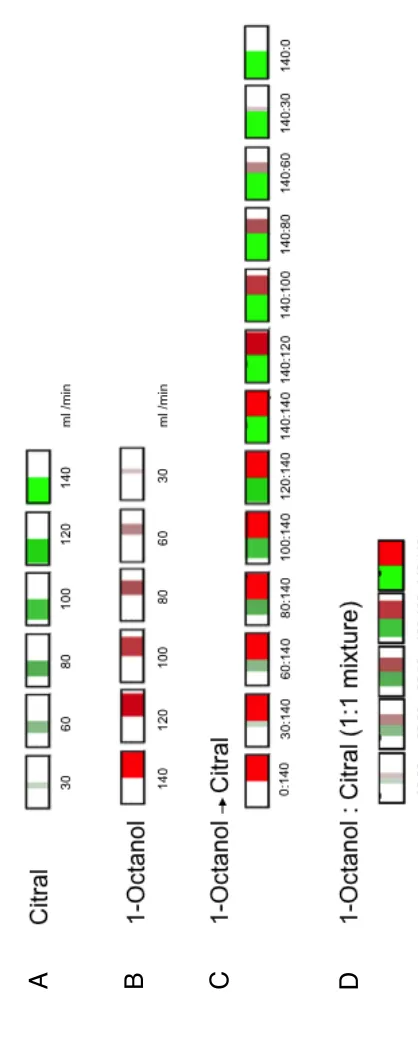
Figure 2.1 Representations of single odors and their mixtures are spread orderly in PN coding space.

A-C. Trajectories representing PN-ensemble responses to binary mixtures. PN activity is

represented as a point in 168-D space, where each dimension represents the firing rate of one of the 168 PNs during one 50-ms time bin. Data analyzed using LLE and projected in the space of the first three LLE components (see Methods). Arrows indicate direction of motion. Three seconds are represented, beginning at odor onset; odor pulses are 300 ms long; each trajectory composed of a sequence of 50ms-bin

measurements, averaged over three trials. (A) PN Population responses to single odors

(citral: green; octanol: red) and to their 1:1 mixture (yellow). Initially at a resting state

(32)

Trajectories to different concentration series of citral, octanol (30, 60, 80, 100, 120, 140 ml/min) and their 1:1 mixture (30:30, 60:60, 80:80, 100:100, 140:140 ml/min). Similar to trajectories for pure odors, concentration-specific trajectories of the 1:1

mixture form odor-specific manifold. Nine-trial averages for each condition. (C)

Trajectories corresponding to odor-morphing series. From Oct to Cit: 140:0, 140:30, 140:60, 140:80, 140:100, 140:120, 140:140, 120:140, 100:140, 80:140, 60:140, 30:140, 0:140. Trajectories change smoothly, with greatest changes away from pure-odor.

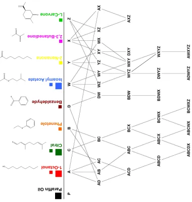
D-H. Multi-component-mixture trajectories (dataset different from that in A-C: 175

other PNs, stimulated with 44 different odor conditions, see Methods). Four and a half seconds are represented, beginning at odor onset; odor pulses: 500 ms long; 50-ms

bins, each averaged over three 2-trial averages. (D) Trajectories in 3-LLE space for the 8

single-odor components. Inset: zoom out of 8 single-odor trajectories together with the 8-mixture trajectory (gray) (LLE axes recalculated). Mixture trajectory loops around

those for individual odors. (E) Starting from single odor W, trajectories increasingly

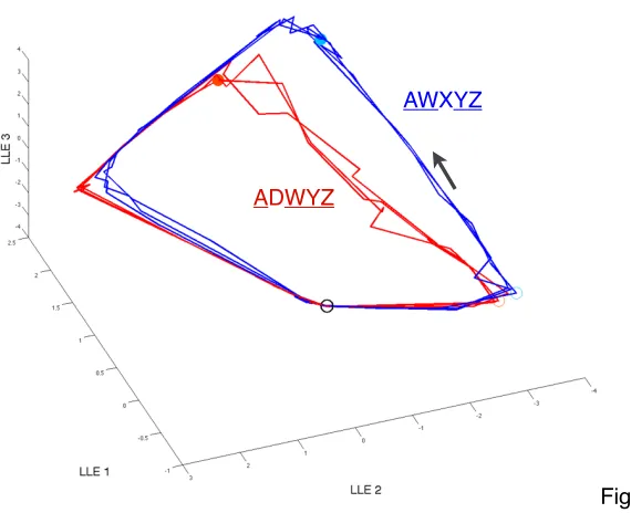
deviate as components added (W→WX→WXY→WXYZ→AWXYZ). (F) Mixtures form

ordered trajectory clusters: family of {W,X,Y,Z} (W, X, Y, Z, WX, WY, WZ, XY, XZ, YZ, WXY, WYZ, WXYZ) well separated from family of {A,B,C,D} (A, B, C, D, AB, AC, AD, BC, ABC,

ACD, ABCD). (G) Trajectories to partly overlapping 4-mixtures. (H) Four D-containing

trajectories (D, AD, ACD, ABCD) plotted together with four Z-containing trajectories (Z, WZ, WYZ, DWYZ). DWYZ trajectory (cyan) follows WYZ trajectory for the most part but deviates towards the D-series transiently. Hence, DWYZ can be classified as related to Z or D, depending on time within response (see text).

I. Minimum correlation distances (dmin) between two trajectories as functions of number

of components in the mixture (correlation distances minimize contributions of firing rate differences). Each bin of a trajectory (2-trial average) is compared with bins of the

other at times t±2bins. Correlation distances in space defined by the 40 first principal

(33)

(34)

2.1.2

Representation of mixtures of increasing

complexity by PNs

We next examined PN trajectories for mixtures of increasing number of

components. Eight molecules were chosen to be chemically distinct and

their concentrations adjusted to evoke minimal, reliable and comparable

electro-antennograms, compensating for differences in vapor pressure or

receptor activation and ensuring operation away from saturation. The

trajectories corresponding to these eight stimuli are shown in Fig. 2.1D.

Consistent with the odors’ distinct chemical composition, these trajectories

did not cluster, indicating large differences between the evoked PN response

patterns.

We first examine the effect of adding 1<n<7 components to a single

odor, W (Fig. 2.1E). The mixture trajectories always deviated from that for W

and from each other. For n>3, however, subsequent component addition led

to decreasing changes in the population trajectory. This is consistent with

the fact that the fractional change to the stimulus decreased with each

single component addition. This observation was repeated with the other

odors and quantified by analysis in the full PN space (not shown).

Second, we observed that, while mixture representations deviated

from those of their components, they still formed clusters of trajectories,

well segregated from those corresponding to non-overlapping mixtures. In

(35)

{W,X,Y,Z} and {A,B,C,,D} are plotted, revealing two non-overlapping

manifolds. This suggests that PN population patterns retain information

about components in mixtures, and that PN trajectories do not spread

randomly in representation space.

Third, we examined the trajectories corresponding to partly

overlapping odors with equivalent strengths (same numbers of

components). In this example (Fig. 2.1G) we plot the trajectories of six

mixtures. Three pairs had an overlap of 3 out of 4 components (BCWX &

BDWX; ABCD & ABCX; WXYZ & DWYZ) and these pairs clearly clustered

together. The other combinations overlapped by two (e.g. BCWX vs. ABCD;

BCWX vs. WXYZ) and were roughly equidistant from one another. This again

suggests an ordered occupancy (qualitatively at least) of PN coding space,

where distances between population representations decrease as

composition overlap increases. Note, however, that overlaps between

mixtures representations—considered until now as averages—often changed

over the course of a trajectory. Figure 2.1H, for example, plots the

trajectories for two groups of odors that were distinct (ABCD vs. WYZ), until

component D was added to WYZ. The addition of D caused a new kink in the

DWYZ trajectory, bringing it closer to the D family during a short segment of

the response. Conversely, two highly overlapping mixtures (overlap of 4 out

of 5 components: ADWYZ and AWXYZ) could be represented by PN

(36)

and then split apart over a later epoch (Fig. S2.8). These results

showed that a fair metric of the similarity between two mixture

representations should be based not on the totality of their corresponding

trajectories, but on piecewise measurements, and on the closest encounter

between them. We thus measured the minimum correlation distances

between every single-component odor and all other odors (other singles,

mixtures of 2, 3, etc.). Using correlation distance (as opposed to Euclidean)

has the advantage of focusing on differences in PN population vectors and

discounting effects attributed to changes in firing rate (such as

concentration). This minimum-distance plot (Fig. 2.1I) was calculated in

three ways: between trials (black), to measure the variance of individual

population representations; between the representations of each single

component and those of all the mixtures containing it (blue); between the

representation of each single component and those of all the mixtures

excluding it (red). The blue and red curves (and corresponding distributions)

were significantly different (Wilcoxon Rank Sum Test, p < 0.01) only for

n=1, 2 or 3. Thus, the representations of a monomolecular odor and of

mixtures of n>3 components are equally distant (on average over odors,

and at the times corresponding to minimum distances) whether the mixture

contains that component of not. In conclusion, while PN-representation

space clearly shows order from mixture coding, extraction of component

composition, based on overlaps between PN population vectors appears

(37)

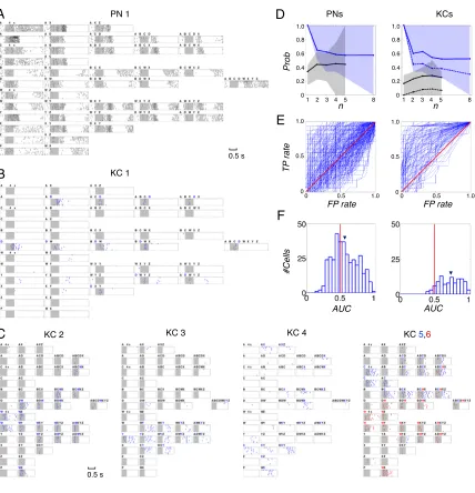
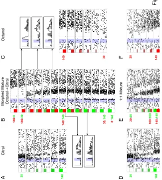
Figure 2.2 KCs segment components out of odor mixtures, but PNs do not.

A. Spike rasters of a representative PN to single and mixed odors (see Methods for 44

stimuli, 7 trials, 500-ms stimulus at shaded area, 2.5 s shown). Numbers of components organized by column, conditions arranged so that overlapping mixtures next to each other wherever possible. Increased inhibition often observed for mixtures

5 4 3 2 1 8 0.6 0.4 0.2 0 1.0 0.8 A B

KC 2 KC 3 KC 4 KC 5,6

KC 1 PN 1 C D E n Pro b PNs KCs n F FP rate FP rate T P ra te AUC #Cells 0.5 s 0.5 s 5 4 3 2 1 8 0.6 0.4 0.2 0 1.0 0.8 0 1.0 0.5 0.5 1.0

0 00 0.5 1.0

1.0

0.5

(38)

with increasing size; responses to mixtures difficult to predict from responses to components (see Fig. S9).

B-C. Spike rasters of six representative KCs (see Figs. S11-14 for more examples). (B)

D-segmenting KC, with weak late response to unrelated mixtures Y, WZ, YZ. Same scale

as in A. (C) Other representative KCs, showing segmentation of different odors (in order

of KCs: W, Y, X, C and W). KCs 5 and 6 recorded simultaneously; both responded to mixtures containing both C and W (e.g., BCWX), but at different times. Only 1 s shown, centered on KC response times; t scale as in B.

D. Conditional probability of response to mixtures, given that cell responds to

components (see text and Method). Blue: “in-class”. Black: “out-class”. Lines: “inclusive”; dashed: “exclusive”. Averaged across all responding cell-odor class pairs. Shaded region: 30-70% distribution. Separation between in-class and out-class much greater for KCs than PNs.

E. ROC evaluation of component selectivity by PNs and KCs. True and false positive rates

(TP, FP) determined by sliding response threshold; response based on spike counts within 1 s window summed over 7 trials. Red diagonal: chance performance. Blue lines: results for each responding cell-odor class pair (see Methods for class partitions).

F. Distribution of area-under-curve (AUC) values for KC-odor class pairs significantly

shifted to the right of PN-odor class pairs (p<3.10-13_{, Wilcoxon rank sum test). Arrows}

indicate means: 0.73 (KCs; SD=0.16); 0.57 (PNs; SD=0.18).

2.1.3

Kenyon cell responses to mixtures

Because Kenyon cells are the direct targets of PNs in the mushroom bodies,

because mushroom bodies are a site for associative memory (48, 80) and

because KC output synapses are plastic (70), KCs are the likely repository of

olfactory memories. It is therefore important to determine the stimulus

features that they extract from PNs. For comparison, we show first the

(39)

(53), this neuron responded to about half of the stimuli with a variety

of discharge patterns (Fig. 2.2A, see also Fig. S2.10). By contrast, KCs

responded very rarely to single odors, but when they did, did so with very

high specificity (Figs. 2.2B-C). Surprisingly, KCs that responded to a

component also often responded to many—if not all—of the mixtures

containing it. KC 1 (Fig. 2.2B), for example, fired in response to odor D, and

responded to all mixtures containing D (though not necessarily at the same

times and for the same durations). The same can be seen with KCs 2 and 6

for odor W (Fig. 2C). KCs 5 and 6 were recorded simultaneously, and each

responded to a different molecule. We found KCs specific to all 8 single

odors. (Our pre-experiment search for KCs always focused on these 8 odors,

but on them only, see Methods; we also found, by chance and thus rarely, a

few KCs specific for binary mixtures; Fig. S2.13). Thus the ability to detect

components in a mixture appears to occur first with KCs.

We next analyzed the difference between PN and KC responses using

two metrics. In the first, we measured conditional probabilities of response

to mixtures, given that a neuron responded to a component (see Methods

for definition of response). If a neuron responded to component c, we

measured the fraction of c-containing mixtures that it responded to (blue

curves). This was repeated for all component-cell combinations with PNs

and KCs (Fig. 2.2D). With KCs, this measurements were performed in two

(40)

one component (continuous lines); an “exclusive” computation

contained KCs that responded to only one component (stippled line); the

later measure is more informative since it excludes the potential

contribution of components other than that tested on responses to

mixtures. This exclusive computation was not possible with PNs for they

always responded to many components. Our second approach was a

receiver-operator-characteristics (ROC) analysis (81), measuring a neuron’s

ability to separate stimuli into “containing-x” and “not-containing-x” sets,

as response threshold is varied. On a true-positive (TP) vs. false-positive

(FP) plot, selective neurons are identified by ROC curves located in the

upper-left quadrant (Fig. 2.2E). Unselective ones run along the diagonal. The

area under the curve (AUC) thus measures selectivity (near 1 for high, near

0.5 for low) (Fig. 2.2F). Both approaches indicated that KCs are significantly

better than PNs at component segmentation. ROC analysis proved that this

is not explained simply by high KC firing thresholds. Hence, in addition to

being highly selective and thus, rare responders, KCs behave as odor

segmenters, extracting component information from PN population vectors.

2.1.4

PN and KC population statistics

We quantified population PN and KC activity as a function of n number of

odor components in the mixture (Fig. S2.17A). Mean baseline PN firing rate

(41)

around odor offset. Peak instantaneous firing (and total spikes)

remained approximately the same as a function n, interestingly, peak firing

rate increased for the higher concentration of single components (~3.8 Hz),

while mixtures of comparable concentration resulted in a lower firing rate

(~2.8 Hz for 4-mixtures, Fig. S2.17A). A closer examination of the response

profiles of firing rates reveals that the onset of firing is earlier for mixtures

than for components, and this difference cannot be accounted for by

concentration alone, e.g., compare peak and onset of 3- mixtures to 4x 1-

components. Next, we examined the percentage of silent PNs as a function

of time and n components. A cell was defined as silent if it fired no spikes

in 100 ms time bins (across 7 trials) to allow for a more conservative

measure of silence. The percentage of silent PNs clearly increases as a

function of n components (Fig. S2.17B). This reflect increased inhibition by

local neurons (LNs) onto PNs. When many components are mixed, this

inhibition is greater for mixtures than for components of comparable

concentrations. Together, these results suggest a gain control mechanism

of mixtures mediated by the PN-LN network that regulates the output of the

PNs. Next, we examined the firing rate of the KC population as a function of

n (Fig. S2.17A), unlike PNs, instantaneous KC firing increases as a function

of n, for ~0.3 Hz for single components to ~0.9 Hz for 8-mixtures. In

addition, we observe that unlike PNs, where many cells become inhibited

during odor response, most KCs by comparison are silent at rest, and a very

(42)

still significant increase in KC firing as a function of n must be

attributed to not greater number of PN spikes, but greater synchrony of PN

inputs.

An important property of neural codes is the activity ratio, the fraction

of active neurons at any one time (82). At one end of the spectrum are local

codes, where each stimulus is represented by a single active cell. At the

other extreme are dense distributed codes, where each stimulus is

represented on average by about half of the cells, e.g., the ASCII code.

Codes with low activity ratios are known as sparse codes, where each

stimulus is represented by much a smaller neuronal population (but not 1

cell), the members of which respond in an explicit manner to specific

features. The activity ratio has implications for coding capacity, memory

recall, generalization, fault tolerance and speed and rules of learning (see Ch

3). Here, we compared the activity ratio between PNs and KCs (Fig. S2.17C).

We measured the responsiveness of cells in short time bins of 50 ms. A cell

was defined as responding if it spiked at least once in 4 of 7 trials, and was

at least 1.5 SDs above the baseline firing (see Methods). At rest, less than

0.4% of all PNs are responding by this metric, however, with odor onset, the

percentage of responsive PNs immediately rose to ~8% for single

components, ~13% for higher concentrations of single components, and

~11% for multi-component mixtures. Because the identities of responding

(43)

responded in at least one time bin (this percentage increased as a

function of n). In comparison, there were no responding KCs at baseline,

and only a very small subset of them responded with odor onset, ~0.5-1% in

any one time bin, and a maximum of ~5% in a 3 s period (to 8- mixture).

These KC response probabilities are qualitatively a 10-, 20- fold

over-estimation, because there was a selective bias for single components in the

KC recordings (see Methods). These results confirm that PN responses are

dense and distributed with a mechanism for gain control of PN outputs. In

contrast, KC responses are sparse and rarely respond (this issue is revisited

in Ch 3). Interestingly, in a recent modeling study (83), it was shown that

optimal discrimination performance is associated with a narrow range of

(44)

Figure 2.3 KCs segment components out of odor mixtures, but PNs do not.

A. Spike rasters of a representative PN to single and mixed odors (see Methods for 44

stimuli, 7 trials, 500-ms stimulus at shaded area, 2.5 s shown). Numbers of components organized by column, conditions arranged so that overlapping mixtures next to each other wherever possible. Increased inhibition often observed for mixtures with increasing size; responses to mixtures difficult to predict from responses to components (see Fig. S9).