Detonation Diffraction Through an Abrupt Area Expansion

Thesis by Eric Schultz

In Partial Fulfillment of the Requirements for the Degree of

Doctor of Philosophy

California Institute of Technology Pasadena, California

2000

Acknowledgments

The efforts of many people have facilitated the research presented in this thesis. Professor Joe Shepherd has served as my advisor, providing me with all of the responsibil-ities and challenges that one could hope for and making this a true learning experience. Pavel Svitek has been an indispensable technician whose contributions can not be over-stated, and many of the experimental facilities were designed and constructed with the help of Joe Haggerty, Larry Frazier, and Ali Kiani in the machine shop. Larry Shaw and Jack Stiles of the Lawrence Livermore National Laboratory helped significantly by pro-viding the framing camera and information necessary to get it running. The assistance and discussions provided by past graduate students, Raza Akbar, Mike Kaneshige, and Chris Krok, past post-doctoral researcher, Julian Lee, and current graduate students, Joanna Austin and Chris Eckett are greatly appreciated. Assistant Professor Andrew Higgins at McGill University has been a reliable source of engagement, ideas, and encouragement throughout my graduate education. My doctoral committee, consisting of Professors Hans Hornung, Brad Sturtevant, Andy Ingersoll, and Jim Beck, deserve my thanks for their input and patience as I have progressed during the past several years. Finally, Suzy Dake has proven to be an invaluable administrative assistant.

Abstract

Contents

1 Introduction . . . 1

2 Literature Review . . . 7

2.1 Shock diffraction . . . 7

2.1.1 Mathematical treatment . . . 7

2.1.2 Qualitative observations. . . 9

2.1.3 Experimental measurements . . . 11

2.2 Detonation diffraction . . . 15

2.2.1 Qualitative observations . . . 15

2.2.2 Experimental measurements . . . 17

2.2.3 Modeling . . . 30

2.2.4 Overviews . . . 34

3 Analytical . . . 37

3.1 Model description . . . 37

3.2 Disturbance propagation . . . 41

3.3 Critical diffraction model. . . 44

4 Computational . . . 55

4.1 Thermochemical equilibrium calculations. . . 58

4.1.1 Specific heat ratio . . . 58

4.1.2 Detonation velocity . . . 62

4.2 ZND detonation simulations . . . 65

4.2.1 Reaction length . . . 68

4.3 Constant-volume explosion simulations . . . 77

4.3.1 Effective activation energy (CJ shock velocity) . . . 79

4.3.2 Critical shock velocity . . . 86

4.3.3 Reaction time . . . 89

4.3.4 Effective activation energy (critical shock velocity) . . . 94

4.4 Non-reacting axial shock decay CFD simulations . . . 100

5 Experimental . . . 105

5.1 Facilities . . . 106

5.2 Diagnostics. . . 108

5.2.1 Pressure transducers . . . 109

5.2.2 Ruby laser shadowgraph . . . 110

5.2.3 Framing camera shadowgraph . . . 110

5.2.4 Digital chemiluminescence imaging . . . 112

5.3 Regime documentation . . . 113

5.4 Disturbance propagation . . . 122

5.5 Axial shock decay . . . 126

5.6 Shock-reaction zone coupling . . . 130

5.7 Critical conditions . . . 136

5.8 Evaluation of the critical diffraction model . . . 138

5.9 Critical diameter correlation with reaction length . . . 151

6 Conclusions . . . 157

7 Recommendations . . . 159

Appendix A Calculated diffraction model parameters . . . 177

Appendix B Conditions from diffraction regime documentation experiments . . 197

Appendix C Images from diffraction regime documentation . . . 199

Appendix D Conditions from critical condition experiments . . . 205

Appendix E Images from critical condition experiments . . . 215

List of Figures

Figure 1.1 Idealized and real detonation waves. ...1

Figure 1.2 Detonation cellular structure. ...3

Figure 1.3 Reaction time sensitivity to shock velocity. ...5

Figure 1.4 Regimes of detonation diffraction. ... 6

Figure 2.1 Qualitative flowfield features of a non-reacting shock diffracting around a corner... 9

Figure 2.2 Diagram of sub-critical diffracting detonation with cellular structure... 16

Figure 2.3 Schematic of equivalent critical tube and critical orifice experiments. ...23

Figure 2.4 Schematic of diffraction experiment with varying divergence angle and ex-pansion ratio. ... 25

Figure 3.1 Schematic model of a diffracting detonation. ...38

Figure 3.2 Schematic of a diffracting non-reacting shock... 41

Figure 3.3 Extension of Skews’ construction to disturbance propagating into a detona-tion front. ...43

Figure 4.1 Simulation-to-experiment induction time deviation for the Konnov (1998) re-action mechanism. ...57

Figure 4.2 Specific heat ratio versus equivalence ratio for fuel-oxygen and fuel-air mix-tures (P₁= 100 kPa, T₁= 295 K). ...59

Figure 4.3 Specific heat ratio versus dilution for stoichiometric hydrogen-oxygen mix-tures (P₁= 100 kPa, T₁= 295 K). ...59

Figure 4.5 Specific heat ratio versus dilution for stoichiometric propane-oxygen mix-tures (P₁= 100 kPa, T₁= 295 K). ... 60 Figure 4.6 Variation of the specific heat ratio function in the critical diameter expression (Eqn 3.46)... 61 Figure 4.7 Detonation velocity versus equivalence ratio for fuel-oxygen and fuel-air

mixtures (P₁= 100 kPa, T₁= 295 K). ... 62 Figure 4.8 Detonation velocity versus initial pressure for stoichiometric fuel-oxygen and fuel-air mixtures (T₁= 295 K). ...63 Figure 4.9 Detonation velocity versus dilution for stoichiometric hydrogen-oxygen mix-tures (P₁= 100 kPa, T₁= 295 K). ... 64 Figure 4.10 Detonation velocity versus dilution for stoichiometric ethylene-oxygen mix-tures (P₁= 100 kPa, T₁= 295 K). ...64 Figure 4.11 Detonation velocity versus dilution for stoichiometric propane-oxygen

mix-tures (P₁= 100 kPa, T₁= 295 K). ... 65 Figure 4.12 Representative steady, one-dimensional detonation simulation. ... 67 Figure 4.13 Detonation reaction length versus equivalence ratio for oxygen and fuel-air mixtures (P₁= 100 kPa, T₁= 295 K). ...69 Figure 4.14 Detonation reaction length versus initial pressure for stoichiometric fuel-ox-ygen and fuel-air mixtures (T₁= 295 K). ...69 Figure 4.15 Detonation reaction length versus dilution for stoichiometric hydrogen-oxy-gen mixtures (P₁= 100 kPa, T₁= 295 K). ...70 Figure 4.16 Detonation reaction length versus dilution for stoichiometric

Figure 4.17 Detonation reaction length versus dilution for stoichiometric propane-oxygen mixtures (P₁= 100 kPa, T₁= 295 K). ...71 Figure 4.18 Disturbance propagation velocity versus time for a representative ZND reac-tion zone computareac-tion. ... 73 Figure 4.19 Disturbance propagation angle versus equivalence ratio for fuel-oxygen mix-tures (P₁= 100 kPa, T₁= 295 K). ...74 Figure 4.20 Disturbance propagation angle versus equivalence ratio for fuel-air mixtures (P₁= 100 kPa, T₁= 295 K). ...74 Figure 4.21 Disturbance propagation angle versus initial pressure for stoichiometric fuel-oxygen mixtures (T₁= 295 K). ...75 Figure 4.22 Disturbance propagation angle versus initial pressure for stoichiometric fuel-air mixtures (T₁= 295 K). ...75 Figure 4.23 Disturbance propagation angle versus dilution for stoichiometric

hydrogen-oxygen mixtures (P₁= 100 kPa, T₁= 295 K). ... 76 Figure 4.24 Disturbance propagation angle versus dilution for stoichiometric

ethylene-oxygen mixtures (P₁= 100 kPa, T₁= 295 K). ...76 Figure 4.25 Disturbance propagation angle versus dilution for stoichiometric propane-ox-ygen mixtures (P₁= 100 kPa, T₁= 295 K). ... 77 Figure 4.26 Representative constant-volume explosion simulation results... 80 Figure 4.27 Activation energy parameter (CJ velocity) versus equivalence ratio for

fuel-oxygen and fuel-air mixtures (P₁= 100 kPa, T₁= 295 K). ...83 Figure 4.28 Activation energy parameter (CJ velocity) versus initial pressure for

Figure 4.29 Activation energy parameter (CJ velocity) versus dilution for stoichiometric hydrogen-oxygen mixtures (P₁= 100 kPa, T₁= 295 K). ...85 Figure 4.30 Activation energy parameter (CJ velocity) versus dilution for stoichiometric ethylene-oxygen mixtures (P₁= 100 kPa, T₁= 295 K). ... 85 Figure 4.31 Activation energy parameter (CJ velocity) versus dilution for stoichiometric propane-oxygen mixtures (P₁= 100 kPa, T₁= 295 K). ...86 Figure 4.32 Critical shock velocity (He and Clavin 1994) versus equivalence ratio

(P₁= 100 kPa, T₁= 295 K). ... 87 Figure 4.33 Critical shock velocity (He and Clavin 1994) versus initial pressure

(T₁= 295 K). ...87 Figure 4.34 Critical shock velocity (He and Clavin 1994) versus dilution for hydrogen

mixtures (P₁= 100 kPa, T₁= 295 K). ...88 Figure 4.35 Critical shock velocity (He and Clavin 1994) versus dilution for ethylene

mixtures (P₁= 100 kPa, T₁= 295 K). ...88 Figure 4.36 Critical shock velocity (He and Clavin 1994) versus dilution for propane mix-tures (P₁= 100 kPa, T₁= 295 K). ... 89 Figure 4.37 Reaction time versus equivalence ratio for oxygen and

hydrogen-air mixtures (P₁= 100 kPa, T₁= 295 K). ...90 Figure 4.38 Reaction time versus equivalence ratio for ethylene-oxygen and ethylene-air mixtures (P₁= 100 kPa, T₁= 295 K). ...90 Figure 4.39 Reaction time versus equivalence ratio for propane-oxygen and propane-air

mixtures (T₁= 295 K). ... 91 Figure 4.41 Reaction time versus initial pressure for ethylene-oxygen and ethylene-air

mixtures (T₁= 295 K). ...92 Figure 4.42 Reaction time versus initial pressure for propane-oxygen and propane-air

mixtures (T₁= 295 K). ...92 Figure 4.43 Reaction time versus dilution for hydrogen mixtures (P₁= 100 kPa,

T₁= 295 K). ...93 Figure 4.44 Reaction time versus dilution for ethylene mixtures (P₁= 100 kPa,

T₁= 295 K). ...93 Figure 4.45 Reaction time versus dilution for propane mixtures (P₁= 100 kPa,

T₁= 295 K)... 94 Figure 4.46 Activation energy parameter (critical velocity) versus equivalence ratio for

hydrogen-oxygen and hydrogen-air mixtures (P₁= 100 kPa, T₁= 295 K). ... 95

Figure 4.47 Activation energy parameter (critical velocity) versus equivalence ratio for ethylene-oxygen and ethylene-air mixtures (P₁= 100 kPa, T₁= 295 K). ..96 Figure 4.48 Activation energy parameter (critical velocity) versus equivalence ratio for

pro-pane-oxygen and propane-air mixtures (T₁= 295 K). ...98 Figure 4.52 Activation energy parameter (critical velocity) versus dilution for hydrogen mixtures (P₁= 100 kPa, T₁= 295 K). ... 98 Figure 4.53 Activation energy parameter (critical velocity) versus dilution for ethylene

mixtures (P₁= 100 kPa, T₁= 295 K). ...99 Figure 4.54 Activation energy parameter (critical velocity) versus dilution for propane

mixtures (P₁= 100 kPa, T₁= 295 K). ... 99 Figure 4.55 Pseudo-Schlieren images from a non-reacting, axisymmetric diffraction sim-ulation with an incident shock Mach number of 6. ...101 Figure 4.56 Simulation and modeling calculations of non-reacting axial shock decay fol-lowing diffraction from an abrupt area change. ...103 Figure 5.1 Experimental configuration with 280 mm detonation tube, 25 mm diffraction tube, and test section. ... 106 Figure 5.2 38 mm diffraction tube and test section. ...108 Figure 5.3 Ruby laser shadowgraph. ... 111 Figure 5.4 Beckman and Whitley 189 framing camera used in shadowgraph

system... 112 Figure 5.5 Shadowgraphs of super-critical detonation diffraction (30 kPa C₂H₂+2.5O₂).

114

(100 kPa 2H₂+O₂). ...119

Figure 5.10 Pressure versus time data for near-critical detonation diffraction... 120

Figure 5.11 Representative framing camera movie of disturbance propagating into planar detonation in H₂+ 0.5O₂+ 0.5N₂ 100kPa mixture (Shot 1093). ... 122

Figure 5.12 Illustration of disturbance propagation measurements from framing camera shadowgraph images. ... 123

Figure 5.13 Worst case disturbance propagation calculations and experimental measure-ments. ...124

Figure 5.14 Best case disturbance propagation calculations and experimental measure-ments. ...124

Figure 5.15 Difference between calculated and experimental disturbance propagation an-gle. ... 125

Figure 5.16 Percentage difference between calculated and experimental disturbance prop-agation angle. ... 125

Figure 5.17 Axial shock decay measurements from Edwards et al. (1979, 1981) detona-tion diffracdetona-tion experiments. ...127

Figure 5.18 Axial shock decay measurements from Ungut et al. (1984) detonation diffrac-tion experiments. ... 128

Figure 5.19 Axial shock velocity decay measurements prior to re-initiation. ...130

Figure 5.20 Super-critical images. ...131

Figure 5.21 Sub-critical images. ...132

Figure 5.22 Near-critical images. ...134

Figure 5.24 Digital chemiluminescence images near the critical time. ...136 Figure 5.25 Critical diameter versus equivalence ratio model and experimental data for

hydrogen-oxygen and hydrogen-air mixtures (P₁= 100 kPa). ...138 Figure 5.26 Critical diameter versus equivalence ratio model and experimental data for

ethylene-oxygen and ethylene-air mixtures (P₁= 100 kPa). ...139 Figure 5.27 Critical diameter versus equivalence ratio model and experimental data for

propane-oxygen and propane-air mixtures (P₁= 100 kPa). ...139 Figure 5.28 Critical diameter versus initial pressure model and experimental data for

sto-ichiometric hydrogen-oxygen and hydrogen-air mixtures. ...140 Figure 5.29 Critical diameter versus initial pressure model and experimental data for

sto-ichiometric ethylene-oxygen and ethylene-air mixtures. ... 141 Figure 5.30 Critical diameter versus initial pressure model and experimental data for

sto-ichiometric propane-oxygen and propane-air mixtures. ... 141 Figure 5.31 Critical diameter versus dilution model and experimental data for

stoichio-metric hydrogen-oxygen-nitrogen mixtures (P₁= 100 kPa). ...143 Figure 5.32 Critical diameter versus dilution model and experimental data for

stoichio-metric ethylene-oxygen-nitrogen mixtures (P₁= 100 kPa). ...143 Figure 5.33 Critical diameter versus dilution model and experimental data for

Figure 5.36 Logarithmic error between model evaluated with He and Clavin (1994) criti-cal shock velocity and experimental criticriti-cal diameter data. ...148 Figure 5.37 Logarithmic error between model evaluated with 0.9V_CJ critical shock veloc-ity and experimental critical diameter data. ... 148 Figure 5.38 Critical diameter versus reaction length correlation for fuel-oxygen mixtures with varying equivalence ratio (P₁= 100 kPa, T₁= 295 K). ...152 Figure 5.39 Critical diameter versus reaction length correlation for fuel-air mixtures with varying equivalence ratio (P₁= 100 kPa, T₁= 295 K). ...152 Figure 5.40 Critical diameter versus reaction length correlation for fuel-oxygen mixtures with varying initial pressure (T₁= 295 K). ...153 Figure 5.41 Critical diameter versus reaction length correlation for hydrogen mixtures

with varying dilution (P₁= 100 kPa, T₁= 295 K). ...153 Figure 5.42 Critical diameter versus reaction length correlation for ethylene mixtures

with varying dilution (P₁= 100 kPa, T₁= 295 K). ...154 Figure 5.43 Critical diameter versus reaction length correlation for propane mixtures with varying dilution (P₁= 100 kPa, T₁= 295 K). ... 154 Figure 5.44 Experimental critical diameter versus detonation reaction length for all

List of Tables

Table 2.1 Sources of critical diffraction conditions. ...18 Table 5.1 Logarithmic error between diffraction model evaluated with He and Clavin

(1994) critical shock velocity and experimental critical diameter data. ...146 Table 5.2 Logarithmic error between diffraction model evaluated with 0.9V_CJ critical

shock velocity and experimental critical diameter data. ...147 Table A.1 Diffraction model parameters for hydrogen-oxygen mixtures with varying

equivalence ratio (P₁= 100 kPa). ...177 Table A.2 Diffraction model parameters for hydrogen-air mixtures with varying equiv-alence ratio (P₁= 100 kPa). ...178 Table A.3 Diffraction model parameters for stoichiometric hydrogen-oxygen mixtures with varying initial pressure... 179 Table A.4 Diffraction model parameters for stoichiometric hydrogen-air mixtures with varying initial pressure. ... 179 Table A.5 Diffraction model parameters for stoichiometric hydrogen-oxygen-argon

mixtures with varying dilution (P₁= 100 kPa). ... 180 Table A.6 Diffraction model parameters for stoichiometric hydrogen-oxygen-carbon di-oxide mixtures with varying dilution (P₁= 100 kPa). ... 181 Table A.7 Diffraction model parameters for stoichiometric hydrogen-oxygen-helium

mixtures with varying dilution (P₁= 100 kPa). ...182 Table A.8 Diffraction model parameters for stoichiometric hydrogen-oxygen-nitrogen

equivalence ratio (P₁= 100 kPa). ...183 Table A.10 Diffraction model parameters for ethylene-air mixtures with varying equiva-lence ratio (P₁= 100 kPa). ...184 Table A.11 Diffraction model parameters for stoichiometric ethylene-oxygen mixtures

with varying initial pressure. ...185 Table A.12 Diffraction model parameters for stoichiometric ethylene-air mixtures with

varying initial pressure. ...186 Table A.13 Diffraction model parameters for stoichiometric ethylene-oxygen-argon mix-tures with varying dilution (P₁= 100 kPa). ...187 Table A.14 Diffraction model parameters for stoichiometric ethylene-oxygen-carbon di-oxide mixtures with varying dilution (P₁= 100 kPa). ...187 Table A.15 Diffraction model parameters for stoichiometric ethylene-oxygen-helium

mixtures with varying dilution (P₁= 100 kPa). ...188 Table A.16 Diffraction model parameters for stoichiometric ethylene-oxygen-nitrogen

mixtures with varying dilution (P₁= 100 kPa). ...189 Table A.17 Diffraction model parameters for propane-oxygen mixtures with varying

equivalence ratio (P₁= 100 kPa). ...190 Table A.18 Diffraction model parameters for propane-air mixtures with varying

equiva-lence ratio (P₁= 100 kPa). ...191 Table A.19 Diffraction model parameters for stoichiometric propane-oxygen mixtures

with varying initial pressure... 192 Table A.20 Diffraction model parameters for stoichiometric propane-air mixtures with

Table A.21 Diffraction model parameters for stoichiometric propane-oxygen-argon mix-tures with varying dilution (P₁= 100 kPa). ...193 Table A.22 Diffraction model parameters for stoichiometric propane-oxygen-carbon

di-oxide mixtures with varying dilution (P₁= 100 kPa). ...194 Table A.23 Diffraction model parameters for stoichiometric propane-oxygen-helium

mixtures with varying dilution (P₁= 100 kPa). ...195 Table A.24 Diffraction model parameters for stoichiometric propane-oxygen-nitrogen

mixtures with varying dilution (P₁= 100 kPa). ...195 Table B.1 Conditions from diffraction regime documentation experiments with stoichi-ometric acetylene-oxygen mixtures. ... 197 Table B.2 Conditions from diffraction regime documentation experiments with stoichi-ometric acetylene-oxygen-argon mixtures. ...197 Table B.3 Conditions from diffraction regime documentation experiments with stoichi-ometric hydrogen-oxygen mixtures. ...198 Table B.4 Conditions from diffraction regime documentation experiments with stoichi-ometric hydrogen-oxygen-nitrogen mixtures (P₁= 100 kPa). ...198 Table D.1 Conditions from critical condition experiments with stoichiometric

hydro-gen-oxygen mixtures, P₁= 100 kPa (common experiments). ...205 Table D.2 Conditions from critical condition experiments with hydrogen-oxygen

mix-tures with varying equivalence ratio. ...206 Table D.3 Conditions from critical condition experiments with stoichiometric

hydro-gen-oxygen-argon mixtures with varying dilution. ...208 Table D.5 Conditions from critical condition experiments with stoichiometric

hydro-gen-oxygen-carbon dioxide mixtures with varying dilution. ...209 Table D.6 Conditions from critical condition experiments with stoichiometric

hydro-gen-oxygen-helium mixtures with varying dilution. ...209 Table D.7 Conditions from critical condition experiments with stoichiometric

hydro-gen-oxygen-nitrogen mixtures with varying dilution... 210 Table D.8 Conditions from critical condition experiments with ethylene-oxygen

mix-tures with varying equivalence ratio. ...210 Table D.9 Conditions from critical condition experiments with stoichiometric ethylene-oxygen mixtures with varying initial pressure. ... 211 Table D.10 Conditions from critical condition experiments with stoichiometric ethylene-oxygen-argon mixtures with varying dilution. ...211 Table D.11 Conditions from critical condition experiments with stoichiometric ethylene-oxygen-carbon dioxide mixtures with varying dilution. ... 211 Table D.12 Conditions from critical condition experiments with stoichiometric ethylene-oxygen-helium mixtures with varying dilution. ... 212 Table D.13 Conditions from critical condition experiments with stoichiometric ethylene-oxygen-nitrogen mixtures with varying dilution. ...212 Table D.14 Conditions from critical condition experiments with stoichiometric propane-oxygen mixtures, P₁= 100 kPa (common experiments)... 212 Table D.15 Conditions from critical condition experiments with propane-oxygen

Table D.16 Conditions from critical condition experiments with stoichiometric propane-oxygen mixtures with varying initial pressure. ...213 Table D.17 Conditions from critical condition experiments with stoichiometric propane-oxygen-argon mixtures with varying dilution. ... 213 Table D.18 Conditions from critical condition experiments with stoichiometric

propane-oxygen-carbon dioxide mixtures with varying dilution. ...213 Table D.19 Conditions from critical condition experiments with stoichiometric propane-oxygen-helium mixtures with varying dilution. ...214 Table D.20 Conditions from critical condition experiments with stoichiometric propane-oxygen-nitrogen mixtures with varying dilution. ...214 Table F.1 Experimental critical diffraction conditions for hydrogen-oxygen mixtures

with varying equivalence ratio. ... 291 Table F.2 Experimental critical diffraction conditions for hydrogen-air mixtures with

varying equivalence ratio. ... 291 Table F.3 Experimental critical diffraction conditions for hydrogen-oxygen mixtures

with varying initial pressure. ...291 Table F.4 Experimental critical diffraction conditions for hydrogen-oxygen-argon mix-tures with varying dilution. ...292 Table F.5 Experimental critical diffraction conditions for hydrogen-oxygen-carbon

di-oxide mixtures with varying dilution. ...292 Table F.6 Experimental critical diffraction conditions for hydrogen-oxygen-helium

mixtures with varying dilution. ... 292 Table F.8 Experimental critical diffraction conditions for ethylene-oxygen mixtures

with varying equivalence ratio. ... 293 Table F.9 Experimental critical diffraction conditions for ethylene-air mixtures with

varying equivalence ratio. ...294 Table F.10 Experimental critical diffraction conditions for ethylene-oxygen mixtures

with varying initial pressure... 294 Table F.11 Experimental critical diffraction conditions for ethylene-oxygen-argon

mix-tures with varying dilution. ... 294 Table F.12 Experimental critical diffraction conditions for ethylene-oxygen-carbon

di-oxide mixtures with varying dilution. ...295 Table F.13 Experimental critical diffraction conditions for ethylene-oxygen-helium mix-tures with varying dilution. ... 295 Table F.14 Experimental critical diffraction conditions for ethylene-oxygen-nitrogen

mixtures with varying dilution. ...295 Table F.15 Experimental critical diffraction conditions for propane-oxygen mixtures

with varying equivalence ratio. ... 296 Table F.16 Experimental critical diffraction conditions for propane-air mixtures with

varying equivalence ratio. ...297 Table F.17 Experimental critical diffraction conditions for propane-oxygen mixtures

with varying initial pressure... 297 Table F.18 Experimental critical diffraction conditions for propane-oxygen-argon

Table F.19 Experimental critical diffraction conditions for propane-oxygen-carbon diox-ide mixtures with varying dilution. ...297 Table F.20 Experimental critical diffraction conditions for propane-oxygen-helium mix-tures with varying dilution. ... 298 Table F.21 Experimental critical diffraction conditions for propane-oxygen-nitrogen

Nomenclature

α angle between disturbance trajectory and the undiffracted shock normal

∆ reaction length

γ ratio of specific heats

∆h0 reaction energy release

λ detonation cell width

ρ density

τ reaction time

Ω kinetic production rate

σ_i thermicity coefficients

θ non-dimensional effective activation energy

A proportionality constant

c frozen acoustic speed

CJ Chapman-Jouguet state

C_p constant pressure specific heat

C_v constant volume specific heat

d tube diameter

d_c critical tube diameter

e specific internal energy

E_a activation energy

h specific enthalpy

k pre-exponential kinetic rate constant

M Mach number

P pressure

R radial distance

R_g gas constant

s post-shock state

t time

t_c critical time for disturbance to reach tube axis

T temperature

u fluid velocity (lab frame)

U_s shock velocity

v transverse disturbance velocity

V_CJ Chapman-Jouguet detonation velocity

vN von-Neumann post-shock state

w fluid velocity (shock frame)

W molecular mass

x distance

x_c critical distance for disturbance to reach tube axis

y mass fraction

1

Introduction

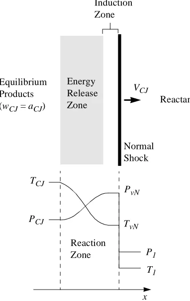
A simple, one-dimensional model of a gaseous detonation, the so-called Zeldov-ich-von Neumann-Doring (ZND) model, consists of a strong shock wave tightly coupled to a reaction zone, propagating through a combustible gas mixture at the Chapman-Jou-guet (CJ) detonation velocity as shown in Fi g.1.1 (Fickett and Davis 1979, Strehlow 1984). Chemical reactions are initiated at the elevated post-shock von Neumann (vN) pressure and temperature. The induction zone behind the shock is usually thermally neu-tral or slightly endothermic as radical species are generated in chain-branching reactions. The temperature increases through the energy release zone as the radical and other inter-mediate species form the primary products in exothermic three-body recombination

reac-Reaction Zone

x P₁

T₁ T_CJ

P_CJ

Normal Shock Equilibrium

Products

(w_CJ= a_CJ) Reactants

Induction Zone

V_CJ

Energy Release Zone

P_vN

T_vN

Figure 1.1 Idealized and real detonation waves. (a) Steady, one-dimensional ZND model.

(b) Laser shadowgraph of self-propa-gating detonation wave

tions. The reaction zone, encompassing the induction and energy release zones,

terminates when chemical equilibrium is reached at the Chapman-Jouguet condition for which the fluid velocity is sonic with respect to the shock wave. Decreasing pressure within the reaction zone arises from expansion of the hot products, emanating compres-sion waves into the adjacent fluid parcels. These comprescompres-sions reinforce the shock wave and counteract momentum and energy loss mechanisms which tend to cause the shock wave to decay. Self-propagating detonation waves exist due to this feedback mechanism wherein the shock wave generates the thermodynamic conditions under which the gas combusts and the energy release from the reaction zone maintains the strength of the shock.

because of the various instability modes which exist (Fickett and Davis 1979), the three-dimensional wave structure is recorded on a two-three-dimensional sheet, and soot foil interpre-tation is quite subjective. Strehlow (1968) classified the observed cellular structure into various qualitative categories such as poor, irregular, good, and excellent. Shepherd et al. (1986a) collected statistical measurements of soot foil cell widths using a digital analysis

l

λ Cell Width

Cell Length

Triple Point Tracks

(b) Laser shadowgraph (H₂+ 0.5O₂+ 10Ar,

P₁= 20 kPa, Akbar 1997) (a) Schematic of cellular structure.

(c) Soot foil recording of cellular structure (C₃H₈+ 5O₂+ 10N₂, P₁= 40 kPa)

technique, quantifying the wavelength spectrum for different mixtures. Those with nar-row spectral content are referred to as having regular cellular structure, while irregular structure is characterized by a broad range of cell widths. Note that cellular structure is present in Fig. 1.1b but the instability wavelengths are small and the wave appears planar.

A detonation propagating from the confinement of a tube into an unconfined space diffracts upon reaching the area change. Expansion waves propagate at a finite rate along the detonation wave and into the fluid behind the wavefront as the presence of the corner is communicated through the flowfield. The diverging streamtubes induced by this distur-bance generate unsteadiness and curvature which reduce the pressure and temperature of the fluid. The chemical reaction rates responsible for the energy release which sustains the detonation are dependent upon these thermodynamic conditions. The time required for a fluid particle to react following the shock can be approximately modeled over a range of temperatures relevant to gaseous detonations by the Arrhenius expression

from which it can be seen that the reaction time is most sensitive to the temperature. Reaction times calculated by constant-volume explosion simulations with varying shock velocity are presented in Fig. 1.3, illustrating the exponential increase in reaction time with decreasing post-shock temperature. Shock velocities ten percent less than V_CJ result in a factor of four increase in reaction time and an order of magnitude or greater reaction time increase with a 15% shock velocity deficit.

The outcome of a detonation wave diffracting from confinement will fall into one of two regimes depending upon the mixture composition, initial thermodynamic state, and

τ k

ρ_s

--- Ea

R_gT_s

--- 

 

exp kRgTs

P_s

--- Ea

R_gT_s

--- 

 

exp

geometry of the confinement (Fig. 1.4). The energy release rate overcomes the expansion rate introduced by the disturbance allowing the detonation to successfully transit the area change in the super-critical regime. Sudden expansion from confinement results in decay of the reaction zone and decoupling from the shock wave in the sub-critical regime. For sufficiently rapid quenching of the reactions, detonation diffraction closely corresponds to self-similar non-reacting shock diffraction. Critical diffraction conditions represent those initial conditions which separate the two regimes. Self-similarity is not present in super-critical cases and near-super-critical conditions due to the influence of the reaction zone.

The fundamental problem of a detonation transitioning from planar to spherical geometry has received considerable attention and has eluded complete understanding in the combustion community for many years. The fluid dynamic complexities associated

Shock Velocity Us/ VCJ

R

eac

ti

o

n

T

im

e

τ

/

τCJ

0.5 0.6 0.7 0.8 0.9 1

100

101 102

103 104

105 106

107

Constant Volume Explosion Simulations Konnov (1998) Reaction Mechanism P₁= 1bar, T₁= 295K

H₂+ 0.5O₂ C₂H₄+ 3O₂ C₃H₈+ 5O₂

with detonation waves, along with the high pressures, high temperatures, and short length/ time scales involved, pose formidable difficulties throughout detonation research. The present investigation is comprised of a combined experimental and analytical approach to characterize the diffraction of gaseous detonations and develop a model which allows for the prediction of critical diffraction conditions. Failure and re-initiation phenomena involved in detonation diffraction are also present in direct initiation, deflagration-to-nation transition (DDT), near-limit propagation, and the self-propagation of cellular deto-nations, and thus, this study sheds light on those problems as well. Beyond the scientific value of this effort, detonation diffraction through area expansions is important in the fields of propulsion, weapons research, and safety/hazard analysis.

d = d_c uCJ

d > d_c uCJ d < d_c uCJ

(a) Supercritical: suc-cessful transmission.

(b) Critical: re-initiation as shock decouples from reaction zone.

(c) Subcritical: complete failure as shock decou-ples from reaction zone.

2

Literature Review

Experimental, analytical, and computational research regarding the problem of detonation diffraction will be reviewed following a summary of some literature on non-reacting shock diffraction. Diffraction in this context is taken to correspond to wave prop-agation in a gaseous mixture through an area expansion, or equivalently, around a convex corner. The efforts of Gvozdeva (1961), Thomas (1979), and Thibault (1985) are

acknowledged, but their publications were not available.

2.1 Shock diffraction

2.1.1 Mathematical treatment

Lighthill (1949) and Chester (1953) treat the problem of a plane shock wave of arbitrary strength moving through gradual area changes by linearizing the governing equa-tions. Resulting shock shapes and pressure distributions were calculated by Lighthill (1949) for shock Mach numbers from one to infinity. Chester (1953) obtained a differen-tial expression for the change in shock strength with area, and provides an analytical expression of the pressure in the disturbance pulse for the cases of subsonic and super-sonic post-shock fluid velocity.

diverging and converging area changes is discussed by Kahane et al. (1954). Idealization of the area change as a step discontinuity along with pressure and velocity matching through shock jump conditions and expansion relations leads to solution of the resulting unsteady wave systems and establishment of steady flow regions.

2.1.2 Qualitative observations

The sketch presented in Fig.2.1 contains many of the flowfield features observed through various experimental efforts. The investigation of Skews (1967a, 1967b) pro-vides an extensive description of the flowfield generated by Mach 1 to 5 shock waves in air diffracting from a rectangular tube through divergence angles of 15° to 165°. Multiple Schlieren images clearly show the propagation of the leading unsteady expansion charac-teristic into the undisturbed incident shock which causes it to diffract. The shape of the unsteady expansion head is indicative of the post-incident shock flow, entirely convected downstream of the area change in the case of post-shock supersonic flow. At relatively high Mach number, a point of inflection was observed between the diffracted shock and

Figure 2.1 Qualitative flowfield features of a non-reacting shock diffracting around a corner.

Incident shock

Contact surface Secondary

shock

Vortex Shear

layer

Unsteady expansion head

Steady expansion

Wall shock

wall shock. A so-called terminator line represents the tail of a steady Prandtl-Meyer expansion, and a shear layer from the separated boundary layer rolls up into a vortex ring. A secondary shock exists near the vortex, and a contact surface is evident which separates the gas processed by the incident shock from that passing through the diffracted shock. All of these features are described in detail by Skews (1967b) along with the variation observed with divergence angle and incident shock Mach number. In particular, a qualita-tive flowfield difference was observed for divergence angles greater and less than 45°. At approximately 45°, the slipstream appears downstream of the corner, with the boundary layer separation point moving closer to the corner with increasing divergence angle. This is accompanied by the contact surface folding under near the wall.

Bazhenova et al. (1971, 1972, 1979) conducted shock diffraction experiments in air, nitrogen, and carbon dioxide from a square shock tube with incident shock Mach num-bers from 1.8 to 10 and divergence angles from 15° to 170°. They provide a good qualita-tive description of the flowfield similar to that of Skews (1967b), as does Quirk (1994) who presents a computational fluid dynamic simulation with pseudo-schlieren images of a shock diffracting around a 90° corner. Bazhenova et al. (1979) and Quirk (1994) note the Mach reflection configuration which the wall shock can assume, giving rise to an associ-ated Mach stem, triple point, reflected shock, and slipstream.

within branched ducts, toroidal vortex formation, and the interaction of successive shock waves with the vortex. Oshima et al. (1965) acquired single-sequence Schlieren and inter-ferogram images of shocks diffracting around a 90° corner, and Deckker and Gururaja (1970) present multi-sequence schlieren images of shocks diffracting through a two-dimensional area expansion. Dumitrescu and Predas (1975) acquired Schlieren images of Mach 2 to 2.5 shocks in air diffracting through divergence angles of 45° and 60° with par-ticular attention paid to boundary layer separation and shock-boundary layer interaction. 2.1.3 Experimental measurements

Oshima et al. (1965) studied the relation between distances propagated by the undisturbed incident shock and the wall shock with Schlieren and interferogram images of Mach 1.5 to 2.8 shock waves diffracting from a rectangular shock tube around a 90° cor-ner. At long times the ratio of these distances was constant, but at early times the constant relation, and therefore self-similarity, was not observed. Schlieren images from Skews (1967a) and Bazhenova et al. (1971, 1979) over a wide range of incident shock Mach numbers and divergence angles indicate that the shock shapes are self-similar to within the experimental accuracy because of the linear relation observed between the incident and wall shock Mach numbers.

images for incident shock Mach numbers from 1 to 3.5 and divergence angles of 15° to 165°. Deckker and Gururaja (1970) present data on axial versus wall shock location for divergence angles from 10° to 45° and incident shock Mach numbers less than two. Shock velocity along the axis is also plotted versus axial shock distance for 10° and 20° diver-gence angles. Comparison with calculations based on Chisnell’s (1957) area-shock strength relation indicates that the calculations overpredict the shock attenuation, with bet-ter agreement for weaker incident shocks.

Sloan and Nettleton (1975) investigated the decay of the shock wave along the tube axis for three- and two-dimensional shock diffractions (Mach 1.5 to 2.5 incident shocks) through abrupt area changes from cylindrical and rectangular shock tubes, respec-tively. The location where the axial shock began to decay was accurately predicted with the expression presented by Skews (1967a) and overpredicted by Whitham’s (1957) the-ory by a factor of 1.7 to 2. The axial shock decay rate was faster and spherical symmetry was achieved sooner for the three-dimensional experiments than the two-dimensional experiments with cylindrical symmetry. Chisnell’s (1957) theory was used in conjunction with measurements of axial shock decay to determine the location at which the shock radius of curvature began to increase linearly with distance. This is the location where the decaying shock achieves spherical or cylindrical symmetry, and extrapolation gave the apparent center of curvature about which the symmetrical expansion proceeds. Observa-tions show that symmetry is achieved faster, and the apparent center of curvature moves closer to the area change plane, as the incident shock Mach number increases.

shock Mach number at incident shock Mach numbers less than 3 and vice versa for larger incident shock Mach numbers (Skews 1967a). The data of Bazhenova et al. (1971, 1979) are used to produce an empirical expression for the wall shock Mach number given the incident shock Mach number and divergence angle. The decay of the wall shock was studied by Sloan and Nettleton (1978) for incident shock Mach numbers of 1.5 to 3.5. They develop a model for the wall shock in which the initial wall shock Mach number is given by Whitham (1957), Chisnell’s (1957) theory is used to account for decay due to cylindrical expansion of the wall shock, and Whitham’s (1957) theory corrects for the slight concavity of the experiment side walls. The model accurately reproduced the atten-uation of the wall shock between two locations but overestimates the absolute wall shock Mach number due to discrepancies between the measured and calculated initial Mach number. Bazhenova et al. (1979) focused on the occurrence of wall shock Mach reflec-tions and presented wall shock Mach number and pressure ratio data versus incident shock Mach number over a wide range of divergence angles and Mach numbers.

presents static and dynamic pressure measurements, positive phase duration, and positive phase impulse for various distances and angles from the area change.

2.2 Detonation diffraction

2.2.1 Qualitative observations

Streak camera experiments of Zeldovich et al. (1956) demonstrated diffracting det-onations decaying to a flame under some conditions and continuing as a detonation for other conditions; this was the first documentation of the sub- and super-critical diffraction regimes. With all other conditions held constant, the tube diameter from which the deto-nation diffracted governed which regime occurred. The detodeto-nation wave failed for tube diameters smaller than the critical tube diameter and vice versa for diameters larger than the critical tube diameter (Fig. 1.4). It was noted that in almost all super-critical diffrac-tions, the shock decoupled from the reaction zone near the tube exit plane edge. Mitro-fanov and Soloukhin (1965) used open-shutter photography of the detonation cellular structure and multi-sequence Schlieren imaging to identify the sub-critical and super-criti-cal regimes, finding that the cellular structure disappears completely in the sub-critisuper-criti-cal case. Figure 2.2 illustrates the observed cellular structure behavior during detonation dif-fraction through an abrupt area expansion. The Schlieren framing camera and streak cam-era images of Soloukhin and Ragland (1969) show complete shock wave decoupling from the reaction zone in the sub-critical regime, and re-initiation of the partially decoupled wave by localized explosions in the super-critical regime. Re-initiation never appeared to occur after the unsteady expansion originating at the edges of the exit plane reached the tube axis. They also observed the boundary layer separation from the tube walls and roll-up into a toroidal vortex.

described re-initiation at criticality occurring in the immediate vicinity of the unsteady expansion head intersection with the tube axis. Very fine cellular structure observed after re-initiation is suggestive of an overdriven detonation. Gubin et al. (1982) saw the same indication of an overdriven detonation following re-initiation and reported that the cell width returned to what would be expected for a detonation propagating at V_CJ after some distance. Detonation diffraction experiments with soot foils by Murray and Lee (1983) revealed two re-initiation mechanisms. The first is the aforementioned re-initiation via localized explosions near the undisturbed core of the diffracting detonation, and the sec-ond occurs when the decoupled shock wave reflects from a confining surface of the vol-ume into which the detonation has diffracted.

Moen et al. (1982) acquired chemiluminescence images from a high speed movie camera and described the localized explosions during re-initiation as being located near

Cellular structure indicating triple-point history.

Detonation front consisting of incident shocks, Mach stems, and reflected shocks (transverse waves)

propagating through tube of diameter d.

Diffracted shock decoupling from reaction zone in the absence of cellular structure. Head of unsteady expansion

wave propagating into undisturbed detonation front.

the interaction point between the unsteady expansion head and the planar detonation front. Edwards et al. (1979, 1981) presents streak camera records of the shock velocity along the tube axis versus distance for a sub-critical and a near-critical super-critical experiment. The shock velocity decayed steadily after the unsteady expansion head propagated to the tube axis in the sub-critical case, while the shock velocity dropped to 0.6V_CJ before accel-erating back to V_CJ in the super-critical case. The authors describe these streak records as reminiscent of the shock front behavior in ignition of spherical detonations by a blast wave generated with a concentrated source of energy.

A significant amount of flow visualization data supports the observations summa-rized above. Additional single- and multi-sequence Schlieren and shadowgraph images are presented by Bazhenova et al. (1969), Edwards et al. (1979, 1981), Thomas et al. (1986), Bartlma and Schroder (1986), Sugimara (1995), and Pantow et al. (1996). Streak camera measurements were obtained by Vasileev and Grigoreev (1980), Gubin et al. (1982), and Ungut et al. (1984). Ungut et al. (1984), Thomas et al. (1986), Desbordes and Vachon (1986), Vasileev (1988), Desbordes (1988), and Borisov and Mikhalkin (1989) obtained soot foil records. High speed movie camera images of detonation chemilumines-cence were acquired by Rinnan (1982), Ungut et al. (1984), Benedick et al. (1984), and Moen et al. (1984a, 1984b). Murray and Lee (1983) and Vasileev (1988) recorded addi-tional open-shutter chemiluminosity images.

2.2.2 Experimental measurements

col-Table 2.1: Sources of critical diffraction conditions.

Source Geometry Mixtures Notes

Zeldovich et al. (1956) Circular C₂H₂-O₂-N₂, C₂H₄-O₂, C₃H₆-O₂-N₂, iC₄H₈-O₂, C₅H₁₂-O₂, C₄H₁₀O,H₂ -O₂, C₃H₆O-O₂, C₆H₆-O₂, CH₄-O₂

no wave veloc-ity measure-ments

Friewald and Koch (1963) Circular C₂H₂-O₂-N₂ Mitrofanov and

Soloukhin (1965)

Circular, Rectangular

C₂H₂-O₂

Strehlow and Salm (1976) Rectangular H₂-O₂-Ar thin channel, 10° to 45°

Edwards et al. (1979) Rectangular C₂H₂-O₂

Matsui and Lee (1979) Circular C₂H₂-O₂-N₂, C₂H₄-O₂ -N₂, C₂H₄O-O₂-N₂, C₃H₆ -O₂-N₂, C₂H₆-O₂-N₂, C₃H₈-O₂-N₂, CH₄-O₂-N₂, H₂-O₂-N₂

Vasileev and Grigoreev (1980)

Circular C₂H₂-O₂-N₂

Edwards et al. (1981) Rectangular C₂H₂-O₂, H₂-O₂-Ar, C₂H₆-O₂, CH₄-O₂, C₃H₈ -O₂, C₃H₆O-O₂

Moen et al. (1981) Circular C₂H₄-O₂-N₂

Knystautas et al. (1982) Circular CH₄-O₂-N₂, C₂H₂-O₂-N₂, C₂H₄-O₂-N₂, C₂H₆-O₂ -N₂, C₃H₆-O₂-N₂, C₃H₈ -O₂-N₂, C₄H₁₀-O₂-N₂, MAPP-O₂-N₂

Gubin et al. (1982) Circular H₂-O₂, CH₄-O₂ 45° and 60° Lee et al. (1982) Circular H₂-O₂-N₂, C₂H₂-O₂-N₂,

CH₄-O₂-N₂, C₃H₈-O₂-N₂, C₃H₆-O₂-N₂, C₄H₁₀-O₂ -N₂, C₂H₄-O₂-N₂, C₂H₆ -O₂-N₂

Moen et al. (1982) Circular C₂H₄-O₂-N₂, C₂H₂-O₂-N₂ some orifice data Guirao et al. (1982) Circular H₂-O₂-N₂

Rinnan (1982) Circular,

Rectangular

C₂H₂-O₂-N₂, C₂H₄-O₂-N₂ some orifice and multiple orifice data

Murray and Lee (1983) Circular C₂H₂-O₂ diffraction into cylindrical geometry Ungut et al. (1984) Circular C₂H₆-O₂-N₂, C₃H₈-O₂-N₂

Liu et al. (1984) Circular, Square, Tri-angular, Elliptical

H₂-O₂-N₂, C₂H₄-O₂-N₂ orifice data

Benedick et al. (1984) Rectangular H₂-O₂-N₂, C₂H₄-O₂-N₂ yielding side wall

Knystautas et al. (1984) Circular H₂-O₂-N₂, C₂H₂-O₂-N₂, C₂H₄-O₂-N₂, C₂H₆-O₂ -N₂, C₃H₈-O₂-N₂, C₄H₁₀ -O₂-N₂

Moen et al. (1984a) Circular C₂H₂-O₂-N₂, C₂H₄-O₂ -N₂, C₂H₆-O₂-N₂, C₃H₈ -O₂-N₂, CH₄-O₂-N₂, H₂ -O₂-N₂

Moen et al. (1984b) Circular C₂H₄-O₂-N₂, H₂-O₂ with additives CF₃Br, CF₄, CO₂

Thomas et al. (1986) Rectangular H₂-O₂, C₂H₂-O₂-Ar 0° to 90° Bartlma and Schroder

(1986)

Rectangular C₃H₈-O₂-N₂, C₃H₈-O₂-Ar 15° to 135° Desbordes and Vachon

(1986)

Circular C₂H₂-O₂-Ar some overdriven and orifice data Shepherd et al. (1986a) Circular C₂H₂-O₂-Ar, H₂-O₂-Ar,

C₂H₆-O₂-Ar

Table 2.1: Sources of critical diffraction conditions.

umn indicates the type of cross section of varying size from which the detonation diffracts. Other than the fuel and diluent type, variations of the mixtures typically include stoichi-ometry, dilution level, and initial pressure. Experiments of some researchers fix the tube diameter and identify the critical limits of these mixture properties, while others fix the mixture properties and vary the tube diameter.

Mitrofanov and Soloukhin (1965) found that the critical diameter was equal to thirteen times the cell width for stoichiometric acetylene-oxygen mixtures of varying ini-tial pressure. Edwards et al. (1979, 1981) verified this correlation with cell width for

acet-Moen et al. (1986) Circular, Annular

C₂H₂-O₂-Ar, C₂H₂-O₂ -N₂, C₃H₈-O₂, C₂H₄-O₂ -N₂

some orifice data

Vasileev (1988) Rectangular C₂H₂-O₂ 0° to 90°, some overdriven and orifice data, thin channel

Desbordes (1988) Circular C₂H₂-O₂-Ar overdriven

Desbordes et al. (1993) Circular C₂H₂-O₂-Ar, C₂H₂-O₂ -He, C₂H₂-O₂-Kr

Makris et al. (1994) Circular H₂-O₂, C₂H₄-O₂, C₃H₈ -O₂, CH₄-O₂, C₂H₂-O₂-Ar

orifice data and diffracting into porous media Sugimara (1995) Rectangular C₂H₂-O₂ thin channel, 18°

to 54° Pantow et al. (1996) Rectangular H₂-O₂-Ar, H₂-O₂-N₂

Higgins and Lee (1998) Circular C₃H₈-O₂, H₂-O₂-Ar, C₂H₂-O₂-Ar

orifice data

Schultz and Shepherd (2000)

Circular H₂-O₂-N₂, C₂H₄-O₂-N₂, C₃H₈-O₂-N₂

some two mix-ture data

Table 2.1: Sources of critical diffraction conditions.

ylene mixtures and extended it to hydrogen mixtures. The d_c= 13λ correlation was discussed as universal after Moen et al. (1981) and Knystautas et al. (1982) demonstrated its validity for a variety of fuel-oxygen-nitrogen mixtures at varying levels of dilution and initial pressure. Since then, d_c= 13λ has approximately held for all other critical diameter tests in which a detonation propagating at V_CJ in fuel-oxygen-nitrogen mixtures of vary-ing stoichiometry, dilution, and initial pressure diffracts from a circular tube through an abrupt area expansion into a relatively unconfined space. The correlation is referred to as approximate because of the cellular structure irregularity discussed in Chapter 1. Unfortu-nately, the cellular structure wavelength spectrum for a given mixture is often not reported along with d_c/λ correlations.

The uncertainty associated with cell width measurements is clear from the correla-tions of many investigacorrela-tions. For example, Vasileev and Grigoreev (1980) observe that the critical diameter to cell width ratio is dependent upon initial pressure and that the ratio for acetylene-air mixtures is significantly greater than for acetylene-oxygen mixtures. Edwards et al. (1981) found d_c= 14λ for ethane and propane mixtures, and d_c= 18λ for methane and acetone mixtures. The comparison between critical diameters measured and predicted with a 13λ correlation by Knystautas et al. (1982) tends to be worse when the cell width data of other researchers is used, highlighting the influence of subjective inter-pretation in cell width measurements. Critical diameter to cell width ratios of 14 to 16 were identified by Ungut et al. (1984) in propane and ethane mixture diffractions. Moen et al. (1984a) finds that d_c/λ ranges from 13 to 24 for a variety of fuel-air mixtures.

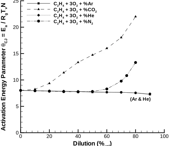
(1986a), and Desbordes et al. (1988, 1993) demonstrated that d_c varied between 4λ and 30λ depending on the type and concentration of diluent. The d_c/λ ratio generally increased with increasing diluent concentration, and this was associated with increasing cellular regularity evaluated subjectively and by Shepherd et al. (1986a) utilizing a digital analysis technique to characterize the cellular structure imprints on soot foils. Moen et al. (1986) claims that relatively low activation energies correspond with increasing mona-tomic dilution of acetylene-oxygen-argon mixtures and cellular regularity. Desbordes (1988) also claims that the activation energy is reduced for heavy argon dilution of acety-lene-oxygen mixtures, and states that this also leads to more stable waves in the context of one-dimensional detonation stability theory (Fickett and Davis 1979). Shepherd et al. (1986a) calculated reaction zone lengths, activation energies, and the overdrive Mach number in which part of the reaction zone becomes endothermic for acetylene, hydrogen, and ethane mixtures diluted with argon, but no clear correlations with cellular regularity were identified. Activation energies were shown not to be significantly smaller for highly argon-diluted mixtures; this is supported by the activation energy data presented in Sec-tion 4.3.1.

spectrum. Therefore, the correlation “constant” of 13 is taken as a ballpark rule-of-thumb value for back of the envelope calculations only, representative when in the context of plus or minus a factor of two for cell width measurements.

Moen et al. (1982) conducted some experiments in which the detonation diffracted through a circular orifice in a plate at the end of a larger diameter tube (Fi g.2.3). They found that the critical orifice diameter was the same as the critical tube diameter for a tube of diameter equal to that of the orifice. The conclusion drawn was that the phenomena governing whether or not a detonation diffraction is sub-critical or super-critical must be local to the wave front because the following flow conditions in critical tube and critical orifice experiments are very different. Experiments by Rinnan (1982), Liu et al. (1984), Desbordes and Vachon (1986), and Vasileev (1988) concur with the equivalence of critical tube and critical orifice diameter. Sugimura (1995) discovered a dependence between the critical initial pressure and orifice plate thickness for detonations expanding into a channel with divergence angles of 18° and 30°. These results indicate that orifice plate experi-ments may be sensitive to the plate thickness and/or that critical orifice experiexperi-ments are not equivalent to critical diameter experiments in which the area change is not abrupt.

The critical channel width for detonations diffracting from rectangular tubes was identified as approximately ten cell widths by Mitrofanov and Soloukhin (1965) and

Figure 2.3 Schematic of equivalent critical tube and critical orifice experiments. (a) Tube diameter d. (b) Orifice plate diameter d.

Edwards et al. (1979, 1981) for acetylene and hydrogen mixtures. Edwards et al. (1981) obtained a critical channel to cell width ratio of 14 for ethane and propane mixtures, and a ratio of 18 for methane and acetone mixtures. They note that a high degree of cellular irregularity and boundary layer influence in their narrow channel experiments could be responsible for the inequality of these ratios. Orifice plate experiments of Liu et al. (1984) included rectangular, square, triangular, and elliptical orifices. The latter three geometries produced results which are in agreement with the approximate d_c= 13λ correlation when the diameter is defined as the average of the diameters inscribing and circumscribing the orifice. Rectangular orifice experiments revealed a critical channel width to cell width ratio dependence upon the orifice aspect ratio, decreasing from a ratio of ten for an aspect ratio of one to a ratio of three for aspect ratios greater than seven. Detonation diffraction tests run by Benedick et al. (1984) from rectangular cross section tubes of variable aspect ratio arrived at the same dependence between critical width and aspect ratio. Moen et al. (1986) conducted diffraction experiments through an orifice with annular geometry. For open area ratios between 0.2 and 0.9, super-critical diffractions were obtained under con-ditions when the annulus outer diameter was up to two times less than the critical tube diameter.

The experiments of Strehlow and Salm (1976) in a rectangular channel with expansion divergence angles of 10° to 45° obtained super-critical diffractions at lower ini-tial pressure and corresponding greater cell widths for smaller divergence angles

90°. Vasileev (1988) observed a divergence angle dependence of up to 45° and no vari-ance in the critical conditions thereafter. Vasileev noted that the expansion surface pro-vides a boundary from which the transverse waves can reflect, and that the independence of criticality of the divergence angle may be related to the fact that the transverse wave angle is approximately 30°.

Schultz and Shepherd (2000) identified critical conditions for diffractions through abrupt area changes in which the diffraction tube was filled with a fuel-oxygen mixture and the unconfined volume a fuel-oxygen-nitrogen mixture. This configuration permitted super-critical diffractions to be obtained under conditions in which sub-critical diffrac-tions were observed for the fuel-oxygen-nitrogen mixture filling the entire apparatus. Sochet et al. (1999) also conducted diffraction experiments through mixture gradients with a receptor mixture of air. Detailed measurements were made of the transmitted shock decay and non-dimensional analyses led to collapse of the shock trajectory and pressure data. Makris et al. (1994) considered detonation diffraction through orifice plates into a space filled with the combustible mixture and tightly packed ceramic spheres. Fuel-oxy-gen mixtures with a high degree of cellular irregularity were not influenced by the orifice diameter. Rather, the wave propagation in the porous media was the same as that observed

Figure 2.4 Schematic of diffraction experiment with varying divergence angle and expansion ratio.

δ

through porous media without initial diffraction through an orifice plate. The results in acetylene-oxygen-argon mixtures with enhanced cellular regularity did exhibit a depen-dence upon the orifice diameter.

Results from the diffraction experiments of Vasileev (1988) indicated that repeat experiments conducted near the critical conditions can have sub-critical and super-critical outcomes. Higgins and Lee (1998) and Higgins (1999) performed many critical orifice tests under the same conditions and observed this phenomenon. They quantified the so-called fuzziness of the critical diameter statistically in terms of the observed percentage of repeat experiments resulting in sub-critical and super-critical diffractions. For example, sub-critical and super-critical cases were found for a ±7% variation off the average critical initial pressure value. Systematic influence of cellular regularity on the fuzziness was not identified.

Soloukhin and Ragland (1969), and Bazhenova et al. (1969) concluded that their diffrac-tion experiments involved overdriven detonadiffrac-tion waves from measurements of the corner disturbance propagating into the undisturbed detonation (see Section 3.2).

Experiments in tubes with short length to diameter ratios can inadvertently result in overdriven detonation diffraction, especially when a deflagration to detonation initia-tion technique is used. Overdriven waves which take some time to decay to V_CJ are a product of DDT initiation just as is observed during re-initiation processes in diffraction experiments. The efforts of Knystautas et al. (1982), Moen et al. (1982), Guirao et al. (1982), Rinnan (1982), Ungut et al. (1984), Moen et al. (1984a), and Moen et al. (1984b) involved diffraction tubes with length to diameter ratios less than 20, and sometimes less than 10. Techniques used to alleviate the uncertainty of detonation overdrive include direct detonation initiation by a powerful ignition source, careful monitoring of the deto-nation wave velocity before it diffracts, and varying the initiator configuration or tube length to check indirectly for an effect of overdrive on the critical conditions. Note that detonation wave velocities were not even measured by Zeldovich et al. (1956).

by boundary layer effects and transverse wave damping in the narrow dimension. The effect of boundary layers also can not be discounted in the experiments of Vasileev and Grigoreev (1980) with tube diameters down to 2 mm.

Murray and Lee (1983) and Thomas et al. (1986) noticed that one detonation re-initiation mechanism during diffraction involves reflection of the decoupled shock wave from a rigid wall of the expansion chamber. This phenomenon changes the critical condi-tions, in fact facilitates super-critical diffraccondi-tions, from what would be obtained in diffrac-tion into a truly unconfined space. It is easily discriminated against when some sort of visualization technique is used, but critical conditions have been reported from experi-ments with relatively small expansion ratios (Fig. 2.4) and using only pressure transducer diagnostics. Vasileev (1988) did not observe wall re-initiation in narrow channel tion experiments for channel width ratios greater than three. Rectangular channel diffrac-tion experiments by Pantow et al. (1996) achieved wall re-initiadiffrac-tion up to channel width ratios of five. The circular tube experimental results presented in Chapter 5 are all

obtained with a combination of flow visualization and pressure transducer diagnostics in a facility with an expansion area ratio of 16. There were cases when the pressure transducer indicated a detonation but the imagery indicated that re-initiation occurred due to decou-pled shock interaction with the expansion chamber wall. Some of the critical conditions reported by Zeldovich et al. (1956), Matsui and Lee (1979), Knystautas et al. (1982), and Guirao et al. (1982) were conducted without visualization diagnostics in facilities with expansion area ratios less than 16.

Rag-land (1969) present shock velocities at many radial and azimuthal locations from their Schlieren movies, from which are calculated the post-shock conditions and induction times to support a discussion of detonation failure. Bazhenova et al. (1969) measured wall shock velocities and unsteady expansion disturbance propagation angles with a framing camera shadowgraph system. They note that the sub-critical diffraction process is self-similar due to rapid quenching of chemical reactions and decoupling of the shock wave, supported by shock position data collapsing onto a straight line in radius versus time coor-dinates. Streak camera records of the shock velocity along the wall and symmetry axis are presented by Edwards et al. (1979, 1981) for sub-critical and super-critical diffraction experiments. Ungut et al. (1984) collected similar records with a multi-beam laser Schlieren time-of-flight anemometer. The shock velocity along the tube axis decayed sig-nificantly before accelerating back to the CJ velocity near the critical conditions. Edwards et al. (1981) overlays Schlieren images with shock shape profiles from Whitham’s (1957) theory and finds reasonable agreement which gets worse with increasing time. Pressure measurements are also provided behind the undisturbed and diffracted regions of the deto-nation. Comparison of wave front shapes from Whitham’s (1957) theory and Schlieren images of Ungut et al. (1984) in self-similarity coordinates reveals good agreement, but in contrast to Edwards et al. (1981), shows better correspondence with increasing time.

Vachon (1986) plot the distance from the tube exit to the point where the unsteady expan-sion intersects the tube axis, the axial distance to the re-initiation location, and the radial distance along the side wall to the re-initiation location versus width and shows that these distances seem to be constant until near the critical cell width. Borisov and Mikhalkin (1989) tabulate unsteady expansion disturbance propagation velocities from soot foil dif-fraction experiments and found them to be 3% to 30% greater than that calculated from the Skews expression evaluated at the post-shock condition (Section 3.2). They also pro-vide data on how much the cell width increases before disappearing and the distance that this occurs away from the unsteady expansion head.

2.2.3 Modeling

Soloukhin and Ragland (1969) offer an ad hoc expression giving the maximum post-shock reaction time for coupling of the shock and reaction zone in terms of the shock radius and velocity. Development of the expression involves the assumption that the post-shock gas all lies within a certain distance from the post-shock, and the reaction time must be less than the transit time of a fluid particle through this distance. Evaluation of this expression and validation against experimental data is not available in the literature. Edwards et al. (1979, 1981) present a model for the critical diameter problem based on notions regarding critical shock strength gradients for