Further Development of Synchronous Array Method for Ad Hoc Wireless Networks

Volume 2009, Article ID 873202,14pages doi:10.1155/2009/873202

Research Article

Further Development of Synchronous Array Method for

Ad Hoc Wireless Networks

Yuan Yu,

_{Yi Huang,}

_{Bin Zhao,}

_{and Yingbo Hua}

1_{Department of Electrical Engineering, University of California, Riverside, CA 92521, USA} 2_{Cinea, Inc., 16 S. 17th Street, Richmond, VA 23219, USA}

Correspondence should be addressed to Yingbo Hua,[email protected]

Received 1 February 2008; Revised 10 May 2008; Accepted 22 July 2008

Recommended by Mary Ingram

A further development of the synchronous array method (SAM) as a medium access control scheme for large-scale ad hoc wireless networks is presented. Under SAM, all transmissions of data packets between adjacent nodes are synchronized on a frame-by-frame basis, and the spacing between concurrent cochannel transmissions of data packets is properly controlled. An opportunistic SAM (O-SAM) is presented which allows concurrent cochannel transmissions to be locally adaptive to channel gain variations. A distributed SAM (D-SAM) is discussed that schedules all concurrent cochannel transmissions in a distributed fashion. For networks of low mobility, the control overhead required by SAM can be made much smaller than the payload. By analysis and simulation, the intranetwork throughput of O-SAM and D-SAM is evaluated. The effects of traffic load and multiple antennas on the intranetwork throughput are studied. The throughput of ALOHA is also analyzed and compared with that of O-SAM and D-SAM. By a distance-weighted throughput, a comparison of long distance transmission versus short distance transmission is also presented. The study of D-SAM reveals an important insight into the MSH-DSCH protocol adopted in IEEE 802.16 standards.

Copyright © 2009 Yuan Yu et al. This is an open access article distributed under the Creative Commons Attribution License, which permits unrestricted use, distribution, and reproduction in any medium, provided the original work is properly cited.

1. Introduction

We consider large-scale ad hoc wireless networks of low mobility within a time interval. Depending on applications, this time interval can be on a time scale of minutes, hours, days, or even longer. Such networks include many types of rapidly deployable wireless networks. There are two types of traffic in ad hoc networks. One is internetwork traffic where traffic flows through one or more gateways (also known as access points) to or from a backbone network. The other is intranetwork traffic where traffic stays within the ad hoc network. For internetwork traffic, the aggregated network throughput is obviously upper bounded by the capacity of the gateways. By either throughput or capacity, we mean network spectral efficiency in terms of bits/s/Hz (bits per second per Hertz). More specifically, we will use bits-hop/s/Hz/node and bits-meter/s/Hz/node as the fundamental intranetwork throughput measure [1,2], which will be explained later. The internetwork traffic will not be considered in this paper.

For intranetwork traffic, the achievable network throughput has been a topic of research by information

0 5

10 15

20

xaxis:q

0 5 10 15 20

y_axis: p 0

0.1 0.2 0.3 0.4

Thr

o

ug

hpu

t

(bits-met

er/s/Hz/node)

x: 3

y: 2

z: 0.3303

Figure 1: The throughput in bits-meter/s/Hz/node of a large network of 245 nodes on square grid versus pandqin the SAM protocol [2]. The node density is one. The SNR at each receiver is 40 dB. The channel coefficients are constant.

topology where totalnnodes are inside a unit-area disk and henceρ = n. It is further shown in [1] that if the network topology is random, then the averaged network throughput has an extra penalty factor in the form of 1/logn. Since [1], there have been new findings on the capacity scaling laws of large-scale ad hoc networks in various alternative settings [3–9]. It should be noted that although representing a theoretical challenge to the above-stated scaling law, a result shown in [10] requires extremely-large-scale virtual multiple-input-multiple-output (MIMO) channels and is highly infeasible according to our analysis.

The capacity scaling laws as discussed above only reveal the effect of the network size. The exact throughput of a large network depends on a wide range of factors. Among them, medium access control (MAC) is critically important. Most of the existing MAC schemes for ad hoc networks are variations of the two basic forms: ALOHA [11] and CSMA (carrier sense multiple access). With CSMA, a node can transmit a packet only when there is no other concurrent cochannel transmission within a large radius. The per-link throughput of CSMA diminishes to zero as quickly as the inverse of the number of nodes within the carrier sensing radius. It is useful to note however that CSMA is adopted in IEEE 802.11 standards [12] for small single-hop networks. With ALOHA, each node initiates a packet transmission randomly. This packet can be received successfully if the intended receiver is ready and the interference is not too high. Because concurrent cochannel transmissions are allowed by ALOHA, the per link throughput of ALOHA does not reduce to zero as the node density increases. In other words, with ALOHA, the capacity scaling lawc/ρ1/2 _{in bits} meter/s/Hz/node holds for networks of regular topologies. A throughput analysis of ALOHA for large network is available in [13]. The throughput shown in [13] was not maximized over the target SINR ξ. As shown in [14], ξ affects the network throughput significantly and can be optimized in practice. In this paper, we distinguish between

signal-to-interference-and-noise ratio (SINR) and signal-to-noise ratio (SNR).

For many potential applications, ad hoc networks have low mobility during operations, which allows cooperations that are not exploited by ALOHA. In [2], the synchronous array method (SAM) was proposed. The essence of SAM is to partition all links in the network into multiple interleaved subsets of links where each subset of links with desired spacing between them corresponds to a set of concurrent cochannel transmissions. As an example,Figure 1illustrates the impact of the spacing between concurrent cochannel transmissions on the network throughput. For this figure, all nodes are on the square grid. For square topology, the spacing or sparseness is measured by p and q which are the vertical and horizontal spacing units between concurrent cochannel transmitters [2]. Also for this figure, the target SINR ξ (i.e., the required SINR value for a packet to be received successfully) is optimized for each pair of p and

q, the channels are nonfading (complex Gaussian fading channels will be considered in the sequel of this paper), and single omnidirectional antenna is used on each node. We see that the impact of the sparseness is significant. For regular topologies such as square, triangle, and hexagon, the sparseness can also be measured by the ratio fs of the

total number of nodes in the network over the number of nodes that are receiving (or transmitting) in each time-frequency slot. InFigure 1, p = 2 andq = 3 are optimal. The correspondingfsis six. Depending on network topology,

antenna properties, and channel fading characteristics, the optimal value of fs varies. But for regular topologies and

omnidirectional antennas, the optimal value of fshas been

found mostly in the range of four, five, and six [14]. If CSMA is applied, the sparseness of concurrent cochannel transmis-sions would be very large and the network throughput would be far below the peak value shown inFigure 1. The idea of using concurrent cochannel transmissions to improve the network efficiency is gaining more attention [15].

The analysis in [14] shows that the throughput of SAM is significantly (about two times) higher than that of ALOHA. In [16], an opportunistic SAM (O-SAM) was proposed that allows concurrent cochannel transmissions to be locally adaptive to channel gain variations. This idea is similar to one used in a channel-state-dependent ALOHA [17] for a single-hop network. But the context for O-SAM is a multihop network rather than a single-hop network. Since the strongest channel gain within each local area is exploited each time, the throughput of O-SAM is much improved. The effect of using multiple antennas is also considered in [18]. However, all of the existing throughput analyses of ALOHA, SAM, and O-SAM are under a full loading condition where each node always has a packet waiting to be transmitted at any time.

In this paper, we will present several new contributions. The first is a comparison of ALOHA and O-SAM under a more general loading condition. This condition is modeled as the probability ζ that each node has a packet for transmission at any given time. We will reveal that the (ξ

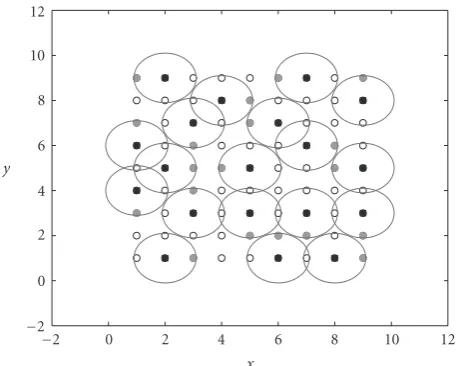
Figure2: Optimal subnet partitions of large networks on regular topologies for O-SAM: the upper left is square, the upper right is hexagon, and the lower is triangle. The sparseness factor fsis five

for the square and triangle topologies and four for the hexagonal topology. The black nodes are concurrent cochannel receivers. One of the blank nodes in each subnet can be a transmitter in that subnet.

comparison of longer-distance transmission versus shortest-distance transmission in terms of the shortest-distance-weighted throughput in bits-meter/s/Hz/node, which shows that the former is worse than the latter unless ζ is very small (e.g., less than 1%). The third is an analysis of O-SAM for the case of multiple antennas on each node, which is an extension of that in [16,18]. The forth is an introduction and evaluation of a distributed SAM (D-SAM) which allows all concurrent cochannel transmissions to be scheduled in a distributed and dynamic way. The essence of D-SAM is similar to that of MSH-DSCH in IEEE 802.16 standards [19]. However, there has been no prior study of the fundamental throughput of MSH-DSCH in large networks. The understanding of D-SAM for large networks can serve this purpose. The study shown in [20] focuses on the dynamic of control packet exchanges, which as explained later does not reveal the fundamental throughput of a network of low mobility. By simulation, we will show the effect of a cooperative radius

R on the throughput of D-SAM. Within the radius R

centered at a receiver, only the desired transmitter is allowed to transmit a data packet. It is important to note that the cooperative radiusRis smaller than an eavesdropping radius

Re. The latter defines the maximum distance between any

two nodes which can eavesdrop each other. Furthermore, a carrier sensing radius Rc would be much larger than the

eavesdropping radiusRe. This study interestingly supports

that the two-hop rule adopted in MSH-DSCH (i.e., all interfering transmitters to a receiver are kept two hops away from the receiver) is a good choice for regular or near-regular topologies under a full load condition. This study also provides a corresponding guidance for choosing a proper packet spectral efficiency, which is not available in IEEE 802.16.

The principle of D-SAM differs from that of a distributed and cooperative link scheduling (DCLS) algorithm shown in [21]. The former is based on the distance information of

neighboring nodes. But the latter is based on calibration of actual SINR for each link. For environment where distance does not well reflect signal attenuation, DCLS could be a better alternative. A detailed comparison between D-SAM and DCLS is not yet available.

Whenever feasible, analysis is given. Otherwise, only sim-ulation is provided. We will measure network throughput by bits-meter/s/Hz/node. All numerical examples to be shown are useful fundamental benchmarks for large networks.

The reminder of this paper is organized as follows. In

Section 2, we extend O-SAM presented in [18] by taking into

account the loading probability ζ. InSection 3, we analyze the network throughput of O-SAM, where the single-input-single-output (SISO), single-input-multiple-output (SIMO), and multiple-input-multiple-output (MIMO) channels are all considered. InSection 4, we present D-SAM in detail. In

Section 5, we revisit the slotted ALOHA with consideration

of the loading probability ζ. In Section 6, we evaluate and compare the network throughput of ALOHA, O-SAM, and D-SAM.

2. Opportunistic SAM

2.1. Subnet Partitions. As mentioned before, the essence of SAM proposed in [2] is to partition all links in the network into multiple interleaved subsets of links where each subset of links with desired spacing between them corresponds to a set of concurrent cochannel transmissions. An equivalent description of SAM is that in any given time-frequency slot, the entire network is partitioned into contiguous subnets and each subnet consists of a receiving node, a transmitting node and possibly several idle nodes. In different time-frequency slots, the corresponding partitions of subnets are relatively shifted from each other.

Figure 2 illustrates the partitions of subsets for square,

triangle and hexagonal topologies. For opportunistic SAM (O-SAM), each receiving node is chosen to be at the center of each subnet, and the transmitting node in each subnet is opportunistically selected from other nodes in the subnet. This is different from SAM in [2] which will also be referred to as centralized SAM (C-SAM) where both receiving and transmitting nodes in each subnet are predetermined.

For the O-SAM protocol shown next and the Gaussian fading channels, the subnet partitions shown inFigure 2have been found to be optimal among other possible partitions. It is useful to note that except for the hexagonal topology, the subnet partitions shown in this figure are not exactly the same as the optimal ones for C-SAM as shown in [14]. But the fact that the optimal subnet partition for the hexagonal topology is the same for both C-SAM and O-SAM makes the hexagonal topology more interesting. This is because the throughput gain by O-SAM via opportunistic selection of transmitters is no longer compromised by altering the subnet partition from the optimal one determined by C-SAM. This advantage will be illustrated numerically later.

time-frequency frame. For a large network, almost all subnets can be treated like a subnet in the center of the network. We will refer to such a subnet as subnet 0 and any other subnet as subnetjwithj=1, 2,. . .,S. We letI0denote the set of the indices of all potential transmitting nodes that have packets to transmit to the receiver in subnet 0. We letn0be the total number of nodes, other than the receiver, in subnet 0. Since

ζ is the probability that a node has a packet to transmit to another node, the probability that I0 contains k nodes is

ζk_(1−ζ)n0−k_{. Note that the setI}

0 is a random set in each time-frequency frame.

2.2.1. SISO Channels. If the channel between every two nodes is modeled as SISO channel, the channel coefficient from theith node inI0to its receiver is denoted byh0,0(i). The corresponding channel gain isv0,0(i)= |h0,0(i)|2_{. The index} of the node with the strongest gain in subnet 0 is denoted by

i0,max=arg maxi∈I0v0,0(i). The index of the node selected for

transmission in subnet 0 is

k0=

i0,max ifv0,0(i0,max)≥θ,

{∅} otherwise. (1)

Here, no node is selected for transmission in subnet 0 if the gain of the node with the strongest gain in the subnet is less than a prespecified threshold θ. The reason behind the use of θ is that if the strongest gain in a subnet is too small, abandoning packet transmission in this subnet causes little loss of information in this subnet and at the same time reduces interference to other subnets. A significant impact of

θon the network throughput under a full load condition was illustrated in [16].

The O-SAM protocol (1) requires each subnet to know the channel gains of all potential transmitting nodes in the subnet. This requires channel estimation and associated exchanges of control packets. This task is feasible if the channel coherence time is relatively long. In fact, for networks of low mobility, the channel coherence time can be very large (e.g., many milliseconds). In this case, only a small fraction (e.g., a few micro seconds) of the channel coherence time needs to be spent for channel estimation. Clearly, the more coordinated is the channel estimation in all subnets, the less time is needed. We will not further address the implementation issues of channel estimation for O-SAM. On the other hand, if the channel gains do not change over time, there is no opportunity to be exploited by O-SAM and the protocol (1) is not meaningful. But random changes in channel gains can be induced artificially if they are not present naturally. To induce random channel gains, one can use multiple transmit antennas on each node and choose a transmit beam vector for each node randomly from frame to frame. This technique also applies to the SIMO and MIMO cases discussed below. The key is to compress the dimension of the channel responses randomly at the transmitter side.

2.2.2. SIMO Channels. If each transmitting node uses one antenna and each receiving node uses multiple antennas, we have a SIMO channel between each transmitter and its receiver. In this case, we define the O-SAM protocol as (1)

except that we usev0,0(i) = h0,0(i)2 _{where h0,0(i) is the} channel response vector between theith node inI0 and its receiver.

We will skip the MISO case since it is similar to the SIMO case.

2.2.3. MIMO Channels. If each node has multiple transmit antennas and multiple receive antennas, we have a MIMO channel between each transmitter and its receiver. In this case, we define the O-SAM protocol as (1) except that

v0,0(i)= λmax(H0,0(i)HH0,0(i)) whereλmaxdenotes the largest eigenvalue and H0,0(i) is the channel response matrix between theith node inI0 and its receiver. The use ofλmax implies that the principal stream of each MIMO channel is used but all other streams are ignored. Because of the interference between concurrent cochannel transmissions, the inclusion of the nonprincipal streams of each MIMO channel into the O-SAM protocol would make the through-put analysis intractable to us at this stage. For this reason, we only consider the principal stream of each MIMO channel.

3. Throughput Analysis of Opportunistic SAM

For throughput analysis, we assume that all elements in channel coefficients, channel response vectors, and channel response matrices are independent and identically dis-tributed (i.i.d.) complex Gaussian random variables. This implies in particular that the channel coefficient between any receive antenna and any transmit antenna is independent of all other channel coefficients.

3.1. SISO Channels. For SISO channels, the signaly0received by the receiving node in subnet 0 can be written as

y0=h0,0x0+

j>0

h0,jxj+w0, (2)

where xj is the transmitted signal from the transmitter

in subnet j, h0,j is the channel coefficient between the

transmitter in subnet jand the receiver in subnet 0, andw0 is white Gaussian noise with zero mean and varianceσ2_{. We} assume thath0,jis complex Gaussian random variable (from

frame to frame) with zero mean and varianceE|h0,j|2=d0,−αj.

Here, α is the path loss exponent and d0,j is the distance

between the transmitter and the receiver. For convenience of analysis, we assume that all nodes transmit with the same powerP, that is,E|xj|2=P. Hence, the instantaneous SINR

at the receiver in subnet 0 is

SINR= v0,0P

j>0v0,jP+σ2

, (3)

wherev0,0 = |h0,0|2 andv0,j = |h0,j|2. We assume that the

to each other. Then, the network throughput in bits-meter/s/Hz/node can be expressed as

CO-SAM=

β

L√ρRξPd, (4)

whereRξ =log₂(1 +ξ) is the packet spectral efficiency, and Pd =Pr{SINR≥ξ}is the probability of a successful packet

detection. Also,Lis the node population in each subnet. As illustrated in Figure 2,L = 5 for the square and triangle topologies, and L = 4 for the hexagonal topology. Finally,

β is a conversion factor from bits/hop/s/Hz/node to bits-meter/s/Hz/node. As shown in [14], we haveβ =0.785 for square topology,β=0.689 for hexagonal topology, andβ= 0.975 for triangle topology. Strictly speaking, the expression (4) is the network throughput for the interior region of the network. For large networks, (4) is a tight lower bound on the network throughput for the entire network.

From the O-SAM protocol, it is clear that the instan-taneous SINR in each time-frequency frame is a random variable that depends onθ andζ, and hence the network throughput is effected byξ,θ, andζ.

In order to evaluate the network throughput (4), we need a more explicit form ofPd, which is derived next:

Pd=Pr{SINR≥ξ,v0,0≥θ}

=Pr

v0,0≥ξ

σ2

P +

j>0

v0,j

, v0,0≥θ

=Pr

j>0

v0,j≤v0,0 ξ −

σ2

P, v0,0≥θ

= ∞ max(ξσ2_/P,θ)

y/ξ−σ2_/P

0 fvI(x)dx

fv0,0(y)d y,

(5)

wherefv0,0(y) is the probability density function (pdf) ofv0,0,

andfvI(x) is the pdf ofvI=

j>0v0,j. Note that the condition

v0,0≥θin the above expression is important. The impact of

θon the network throughput is significant and illustrated in [16] (under the full load condition). In this paper, we will not further illustrate the effect ofθ. Unless mentioned otherwise,

θis optimally chosen to maximize the network throughput. In order to evaluate Pd shown in (5), we need to

obtain the expressions of the two pdf functions fv0,0(y) and fvI(x). We start withfv0,0(y). Since|h0,0(m)|

2_{is exponentially}

distributed with the meanD0,0(m)=d0,0−α(m), whered0,0(m) is the distance between the transmitter and receiver in subnet 0 andαis the path loss exponent, it follows that

Pr{v0,0≤y} =

m∈I0

Pr{v0,0(m)≤y}

=

m∈I0

1−exp

₋

y D0,0(m)

U(y), (6)

whereU(y) is the unit step function. The above expression is not ready to use sinceI0is a random set. Alternatively and equivalently, we can think of a node that has no packet to

transmit as if it is a node that has zero channel gain with respect to the receiver. Following this thinking, we can write

Pr{v0,0≤y} =

n0

m=1

1−exp

₋

y D0,0(m)

ζ+ (1−ζ)

U(y)

=

n0

m=1

1−ζexp

₋

y D0,0(m)

U(y),

(7)

wheren0 is the number of potential transmitters in subnet 0. The pdf fv0,0(y) follows readily from the derivative of

Pr{v0,0≤y}shown in (7), that is,

fv0,0(y)=

n0

k=1

δ(y) +ζ 1 D0,0(k)exp

₋

y D0,0(k)

×

n0

m=1,m /=k

1−ζexp

₋

y D0,0(m)

U(y), (8)

whereδ(y) is the Dirac’s delta function. To derive the pdffvI(x) wherevI=

j>0v0,j, we start with

the following:

Pr{v0,j≤x} =

Pj+ nj

l=1

Pj,lPr{|h0,j(l)|2≤x}

U(x)

=

Pj+ nj

l=1

Pj,l

1−exp

₋

x D0,j(l)

U(x),

(9)

wherePj is the probability that there is no transmission in

subnet j, and Pj,l is the probability that the lth node in

subnet jtransmits. We have usednj to denote the number

of potential transmitters in subnet j. In (9), we also used the property that|h0,j(l)|2is exponentially distributed with the

meanD0,j(l)=d0,−αj(l), whered0,j(l) is the distance between

thelth transmitter in subnetjand the receiver in subnet 0. It follows that

Pj=1−

l Pj,l

Pj,l=ζ·Pr

vj,j(l)≥θ, max k /=l,k∈Ij

vj,j(k)≤vj,j(l)

=ζ ∞

θ

1

Dj,j(l)e

−x/Dj,j(l)

k /=l,k∈{1,2,...,nj}

(1−ζe−x/Dj,j(k)_)dx,

(10)

where we have used the technique used for (7). Then, the pdf

fv0,j(x) follows readily from the derivative of (9), which is a

superimposed-exponential, that is,

fv0,j(x)=Pjδ(x) +

nj

l=1

Pj,l

1

D0,j(l)e

−x/D0,j(l)_{U(x). (11)}

for all j >0. Assume that fvI(x) is negligible forx ≥T. We

can write the Fourier series expansion of fvI(x) as follows:

fvI(x)=

K

k=−K

gkexp

υ2πk T x

, (12)

whereυ=√−1 and

gk=

1

T T

0fvI(t) exp

−υ2πk T t

dt

= 1

T

j>0

Pj+ nj

l=1

Pl j

1 +υ(2πk/T)D0,j(l)

.

(13)

We will assume thatgkis negligible fork > K.

With fv0,0(x) and fvI(x) as shown above,Pdin (5) can be

readily computed.

3.2. SIMO Channels. For SIMO channels where there arenr

receiving antennas at each node, the signal received by the receiver in subnet 0 has the following expression:

y0=h0,0x0+

j>0

h0,jxj+w0. (14)

Here, xi denotes the signal transmitted from subnet i.

hi,j ∈ Cnr×1 is the channel coefficient vector between the

transmitter in subnet j and the receiver in subnet i. The entries inhi,jare assumed to be independent and identically

distributed complex Gaussian random variables with zero mean and variance d−i,jα(kj) where kj is given by (15) and di,j(kj) is the distance between the transmitter in subnet j

and the receiver in subnet i, α is the path loss exponent. wi is the complex noise vector at the receiver in subnet i,

and assumed to have zero mean and the covariance matrix

E{wH

i wi} = σ2Inr where Inr denotes the nr ×nr identity

matrix. We also assume that all the nodes in the network transmit with the same powerP, that is,E{xH

i xi} =P.

It is important to note that based on the O-SAM protocol,hi,j=hi,j(kj) where

kj=arg

max

k∈Ij,hj,j(k)2≥θ

hj,j(k)2

. (15)

Also recall that hi,j(k) is the channel response vector from

thekth potential transmitter in subnet j to the receiver in subneti.

A sufficient statistics ofy0 is given by r0 = hH0,0y0. The SINR inr0is

SINR= h

H

0,0h0,0

j>0(|hH0,0h0,j|2/h0,02) +σ2/P

= v0,0

j>0v0,j+σ2/P

,

(16)

wherev0,0=hH0,0h0,0andv0,j= |hH0,0h0,j|2/h0,02.

Given any h0,0, hj(l) =. h0,0Hh0,j(l)/h0,0 is a linear combination of the elements of h0,j(l) which are i.i.d.

complex Gaussian random variable, and hence hj(l) is a

complex Gaussian variable. Each element ofh0,j(l) has zero

mean and the varianceD0,j(l) = d0,αj(l) whered0,j(l) is the

distance between thelth node in subnet j and the receiver in subnet 0. Furthermore, one can verify as in [22] that

hj(l) has zero mean and the varianceD0,j(l). It follows that v0,j(l) = |hj(l)|2 for j > 0 is independent of h0,0 and is exponentially distributed with meanD0,j(l), that is,

fv0,j(l)(y)=

1

D0,j(l)exp

_−y

D0,j(l)

U(y), j >0. (17)

Sincev0,j=v0,j(kj) withkjgiven by (15),v0,jforj >0 is

also independent ofh0,0.

Therefore, with the above description ofv0,0andv0,j, the

throughput expression (4) and the probability-of-detection expression (5) are also valid for the case of SIMO channels except that the expressions of the pdf fv0,0(y) ofv0,0and the

pdf fvI(x) ofvI=

j>0v0,jneed to be revised as follows.

To find fv0,0(y), we first write

Pr{v0,0≤y} =

n0

m=1

{ζPr(h0,0(m)2_{≤y) + (1−ζ)}U(y).}

(18)

It is known that h0,j(l)2 is Chi-square or gamma

dis-tributed with 2nrdegrees, that is,

fh0,j(l)2(x)=

xnr−1 (nr−1)!Dn0,rj(l)

e−x/D0,j(l)_{U(x). (19)}

Therefore,

Pr{v0,0≤y} =

n0

m=1

ζ y

0

xnr−1 (nr−1)!Dn0,0r(m)

e−x/D0,0(m)_dx

+ (1−ζ)

U(y)

=

n0

m=1

ζ

1−e−y/D0,0(m)

nr−1

k=0

yk Dk

0,0(m)k!

+ 1−ζ

U(y)

=

n0

m=1

1−ζe−y/D0,0(m)_g

_y

D0,0(m)

U(y),

(20)

whereg(y)=nr−1

k=0(yk/k!). The pdf fv0,0(y) is simply given

subnet, that is,Dj,j(m)=Dfor alljand allm, the pdf fv0,0(y)

can be shown to be

fv0,0(y)= ∂

∂yPr{v0,0≤y}

=

n0

μ=1

n0

μ

(−1)μ+1ζμe−(μ/D)ygμ−1

y D

× μynr−1

Dnr₍n

r−1)!U

(y) + (1−ζ)n0 δ(y)

=n0

1−ζe−y/D_g

_y

D

n0−1_ζe−y/D_ynr−1

Dnr(n_r−1)!U(y)

+ (1−ζ)n0 δ(y).

(21)

We now derive the pdf fvI(x) of vI =

j>0v0,j where v0,j= |hH0,0h0,j|2/h0,02. Since the pdf ofv0,j(l) is the same as

that for the SISO channels, all expressions for the pdf fvI(x)

are the same as for the SISO case except thatPj,lneeds to be

revised as follows:

Pj,l=ζ·Pr

hj,j(l)2≥max

k /=lhj,j(k)

2_{, h}

j,j(l)2≥θ

=ζ ∞

θ

xnr−1 (nr−1)!Dnj,rj(l)

e−x/Dj,j(l)

×

k /=l

1−ζe−x/Dj,j(k)

nr−1

q=0

xq Dj,j(k)qq!

dx,

(22)

where we have used (19). IfDj,j(l)=Dfor alljand alll, then Pj,lbecomes independent ofl, andPj,lcan be simplified as

Pj,l=ζ

∞

θ

xnr−1 (nr−1)!Dnre

−x/D

1−ζe−x/D nr−1

q=0

xq Dq_q!

n0−1 dx.

(23)

3.3. MIMO Channels. For MIMO channels, the received signal model in subnet 0 is given by

y0=H0,0x0+

i>0

H0,ixi+w0, (24)

whereHi,j∈Cnr×ntis the channel coefficient vector between

the transmitter in subnet jand the receiver in subneti. The entries inHi,jare assumed to be independent and identically

distributed complex Gaussian random variables with zero mean and variancedi−,jα(kj) withkjdefined by (25).xiis the

complex vector signal transmitted from subneti.wi is the

complex noise vector at the receiver in subneti, and assumed to have zero mean and the covariance matrix E{wHi wi} = σ2_I

nr, whereInr denotes thenr×nridentity matrix. We also

assume that all the nodes in the network transmit with the same powerP, that is, tr{E{xixiH}} =P. We further assume

thatnr=nt.

Based on the O-SAM protocol,Hi,j=Hi,j(kj) where

kj=arg

max

k∈Ij,λmax(Hi,j(k))≥θ

λmax(Hi,j(k))

. (25)

Denote the singular value decomposition (SVD) of Hi,i

as Hi,i = Ui,iΛi1,/i2VHi,i where Λi,i is a diagonal matrix of

nonnegative entries in a descending order. Then, we can transform (24) to the following:

y0=Λ10,0/2x0+

i>0

H0,ixi+w0, (26)

wherey₀ =UH0,0y0,xi =VHi,ixi,H0,i=UH0,0H0,iVi,iandw0 = UH

0,0w0.

Under the O-SAM protocol, we only use the principal stream of each MIMO link. In this case, only the first entry of the vectorxiis nonzero, which is denoted byxi. Therefore, a

sufficient statistics of the vectory0is given by its first element, which is denoted by y0, and (26) is equivalent to the scalar equation

y0=λ1max/2x0+

j>0

h0,jxj+w0, (27)

whereλmaxis the largest eigenvalue ofH0,0HH0,0, andh0,jis the

upper-left entry ofH0,jwhich is complex Gaussian with zero

mean and varianced−0,αj(kj).

The SINR iny0is given by

SINR= v0,0

j>0v0,j+σ2/P

, (28)

wherev0,0 =λmax, andv0,j = |h0,j|2which is exponentially

distributed with the meanD0,j(kj)=d0,−αj(kj).

Assuming thatd0,0(m)=1 for allm=1, 2,. . .,n0, the cdf (cumulative distribution function) ofλmaxis known [23] to be

Fλmax(x)=

1 nr

j=1Γ(j)2

det|(γi+j−2)|, (29)

where (γi+j−2) is a nr ×nr matrix with element γi+j−2 = x

0ωi+j−2exp(−ω)dωandΓ(j)=(j−1)!.

The expressions (4) and (5) still hold for the MIMO case except that fvI(x) andfv0,0(y) need to be revised as follows.

We know that

Pr{v0,0≤y} =

n0

m=1

{ζFλmax(y) + (1−ζ)}

= {ζFλmax(y) + (1−ζ)}

n0_.

(30)

Then, fv0,0(y) is given by the derivative of (30).

The expressions for fvI(x) are the same as those for the

SISO and SIMO cases except that

Pj,l=

1

nj(1−Pj),

Pj=(1−ζ+ζFλmax(θ))

nj_.

Data subframe Control

subframe Initialization Data

subframe Control

subframe Initialization

Framen+ 1 Framen

Contention slot · · ·

Contention slot

Data slot

Data

slot · · ·

Data slot

Figure3: Frame structure of the distributed SAM protocol, which resembles that of MSH-DSCH in IEEE 802.16.

4. Distributed SAM

The (centralized) SAM shown in [2] and the opportunistic SAM shown in Section 2 all require a subnet partition in a centralized fashion. The dimension of each subnet or the spacing between concurrent cochannel transmissions is critical for network throughput. In this section, we present a distributed SAM (D-SAM) that encapsulates an essence of SAM in that all concurrent cochannel transmissions are properly spaced from each other. But D-SAM forms subnets in each time frame in a distributed and dynamic fashion. D-SAM also works with random network topology.

In D-SAM, time is slotted into frames of equal duration as shown in Figure 3. Each frame is further divided into control subframe and data subframe. Assuming that the data subframe is much longer than the control subframe, the network spectral efficiency is dominated by the spectral efficiency in each data subframe. A control subframe is used for each node to compete for data transmission opportunity in a data subframe. Each control subframe consists of a group of M contention slots. For analysis of maximal achievable throughput, we will assume without loss of generality that each data subframe consists of a single data slot.

At the beginning of each frame, D-SAM allows each node to randomly initialize a choice for one of theMcontention slots if the node has a packet to transmit to another node. If the node has packets to be transmitted (separately) to multiple neighboring nodes, the node chooses multiple contention slots, one slot for each receiver. During a chosen contention slot, the node contends for the upcoming data subframe by starting a handshaking process with its intended receiving node. The handshaking involves three packets: request-to-sent (RTS), clear-to-sent (CTS), and ACK. If the handshaking is successful, the upcoming data subframe is reserved for data transmission between the transmitter-and-receiver pair. During each contention slot, the handshaking packets are received by neighboring nodes so that these nodes are aware of the reservation status of the upcoming data frame. For each frame and each neighborhood in a predetermined range, the data subframe can only be reserved for one transmitter-and-receiver pair. This means that the first contention slot has the highest priority, the second contention slot has the second priority, and so on. In the next frame, the contention process repeats without memory of the previous contentions, which ensures fairness.

More details of D-SAM are as follows. We assume that each node k maintains a neighborhood listNk which

contains the identifications of all its neighboring nodes inside a cooperative rangeR. The rangeRis an important parameter for the performance of D-SAM. Theith node in

Nkis indexed byNk(i). The neighborhood list at each node

can be established at the startup of the network. For networks of low mobility, this startup is feasible. We assume that every node can be set to one of three states for the upcoming data subframe:T,R, andS. Here,Tstands for transmitting,Rfor receiving, andSfor standby. We denote the state of nodekas

Skand the state ofNk(i) asSNk(i).

(1) Initialization: At the beginning of each frame, set every node to stateS, that is,Sk=Sfor allk. Then, we allow

that every nodekgenerates a “contention request vector”vk

that randomly maps each neighboring node in listNkto one

ofMcontention slots if nodekhas traffic load intended to those neighbors. Here, we assume thatMis larger than the size of every neighbor list, that is,M ≥ |Nk|for allk. The

ratio ofMover|Nk|affects the probability of handshaking

collisions. The larger is the ratio, the lower is the probability of handshaking collisions. We denote themth element ofvk

asvk(m), which is

vk(m)=

⎧ ⎪ ⎪ ⎨ ⎪ ⎪ ⎩

j if nodek has traffic to node j, and j

is mapped into contention slotm, 0 otherwise.

(32)

In other words, the value of vk(m) is the index of the

receiving node for which the transmitting nodekwants to contend during the contention slot m for the upcoming data subframe. If vk(m) = 0, it means that, in the mth

contention slot, nodekwill not contend for the upcoming data subframe.

(2) In contention slotm: each nodekwill first check its contention request vector. Ifvk(m)= 0, nodekeavesdrops

ongoing handshaking within the neighborhood of range

R. (Naturally, we assume that the eavesdropping range

Re from each node is larger than the cooperative range

R. Furthermore, the carrier sense range Rc, although not

considered in this paper, would be even larger than Re.)

finish the following three-way RTS-CTS-ACK handshaking with node j.

(i) RTS:

Nodeksends an RTS packet to nodejwhich contains the identity of nodek, if the following conditions are satisfied:

(a)Sk=S;

(b)SNk(i)=/Rfor alli.

(ii) CTS:

If node j has successfully received the RTS packet from node k and the following conditions are satisfied:

(a)Sj=S;

(b)SNj(i)=Sfor alli;

(c)vj(m)=0,

then nodejresetsSj=RandSNj(ik)=Twhereikis

the index for nodekin the tableNj, and sends a CTS

packet back to nodek.

(iii) ACK:

If node k has successfully received the CTS packet from nodej, the nodekresetsSk=TandSNk(ij)=R

whereij is the index of node j in the tableNk, and

sends back the ACK packet.

During any contention slot, if there is a collision of control packets within the radiusR, the operation in that slot is abandoned. But the collision of control packets at a receiver due to transmitters outside the radius Ris assumed to be resolvable by using coding with relatively high redundancy. If the ratio ofMover the number of nodes within the radiusR

is large, the probability of collision of control packets is small. As long as the control packets are much smaller than the data packets (i.e., the control subframe is much smaller than the data subframe), the network spectral efficiency is dominated by the throughput in the data subframe. This assumption will be our basis for throughput evaluation of D-SAM.

The idea of using control subframe for scheduling is not new, which can be traced back to the bit map concept as well as the work shown in [24]. But the study of the impact of the cooperative radiusRon the network throughput is new and important for large-scale ad hoc networks.

Figure 4illustrates a snapshot of the concurrent

cochan-nel transmission pairs for a square network, which was determined by D-SAM for data transmission. The radius

R = da was chosen, whereda is the spacing between two

nearest neighbors. The number of contention slots wasM= 8. The full traffic loading condition, that is, ζ = 1, was assumed.

For D-SAM, we evaluate the network throughput in bits-meter/s/Hz/node as follows:

CD-SAM=E

1

N N

n=1

dnRξsn

, (33)

−2 0 2 4 6 8 10 12

x −2

0 2 4 6 8 10 12

y

Figure 4: A snapshot of concurrent cochannel transmissions determined by the D-SAM protocol for a network in a regular square grid.R=da,M=8, andζ=1 were used, wheredais the

minimum distance between two adjacent nodes. The black nodes are the receiving nodes, and the grey nodes are the transmitting nodes.

whereEdenotes expectation,Nis the total number of nodes in the network,dnis the distance between thenth receiving

node and its transmitting node, Rξ is the packet spectral

efficiency as defined before, sn ∈ {0, 1}, and sn = 1 if

and only if a packet is intended for thenth node and the corresponding SINR is no less than ξ. In the simulation, the expectation is replaced by the average over many time frames. Each time frame also corresponds to an independent realization of Gaussian random channels. The distance weighting in (33) is different from the conversion formulas (from bits-hop/s/Hz/node to bits-meter/s/Hz/node) derived in [14] because the former does not take into account the fact that a typical multihop route between source node and destination node is not a straight line due to topology constraint. However, for regular topologies, the weighting used in (33) is slightly larger than that used in [14]. For an arbitrary topology, (33) represents an upper bound on the throughput in bits-meter/s/Hz/node.

5. Loading Adaptive ALOHA

Slotted ALOHA (or ALOHA for short) is a useful benchmark for throughput comparison. The protocol of ALOHA is as follows. In each time slot or frame, if a nodeAhas a packet to deliver to a neighboring nodeB, then the nodeAtransmits the packet to the nodeBwith a transmission probabilityε. If the nodeBis not transmitting in the same time slot, the node

Battempts to receive the packet from the nodeA.

by the following expression [14]:

CALOHA=√β

ρ(1−ζε)ζεRξPd. (34)

Here, as defined before,Rξ is the packet spectral efficiency,

and Pd = Pr{SINR ≥ ξ} is the probability of packet

detection. However, the statistics of SINR for ALOHA is different from that for SAM.

Note that the above expression (34) is for “per node” throughput, that is, in terms of bits-meter/s/Hz/node. (It is per every source node.) If there are totalNnodes whereNis large, the aggregated network throughput in bits-meter/s/Hz isNtimes the expression (34). This expression has taken into account statistically all possible transmission patterns, which include the scenarios where multiple nodes are transmitting to a common receiver. When a node is in the receiving mode, it tries to decode the information from each of its neighboring nodes (say, nodesAandB). When the receiving node tries to decode the information from nodeA, the signal from node B (if any) will be treated as noise, and vice versa. A simple way to understand (34) is to first consider the network throughput in terms of bits-hop/s/Hz/node [2], which corresponds to the (averaged) throughput for each pair of neighboring nodes. The probability that each pair of neighboring nodes forms a transceiver is given by (1−ζε)ζε. Given that a pair of neighboring nodes forms a transceiver, the amount of information transferred between them isRξPd. Hence, (1−ζε)ζεRξPdis the throughput in

bits-hop/s/Hz/node. The factor β/√ρ converts the throughput from bits-hop/s/Hz/node to bits-meter/s/Hz/node, see [14]. Also note that the expression (34) assumes one type of multiuser detection at each receiving node. However, the packets from multiple transmitters are not jointly encoded.

For throughput analysis of ALOHA, we will only consider SISO channels. Then, given that a node transmits a packet and one of its neighboring nodes receives the packet, the signal received by the receiving node can be modeled as

y0=h0x0+

j>0

hjxjuj+w0, (35)

wherex0 is the desired signal,h0 is the channel coefficient between the desired transmitter-receiver pair, xj for j > 0

is the interfering signal from node j,hj for j > 0 is the

channel coefficient between the interfering node j and the receiving node, and w0 is the noise. We assume Gaussian fading channels and Gaussian noise. Here,uj ∈ {0, 1}are

i.i.d. binary random variables with Pr{uj =1} =ζε. Then,

the instantaneous SINR iny0in each time slot is

SINR= g0P

σ2₊

j>0gjujP

, (36)

where P is the transmitted power from each transmitting node,σ2_{is the noise variance,g}

i= hi2is an exponentially

distributed random variable with the meanμi=di−α, anddi

is the distance between the nodeiand the receiver.

Unlike (5), we now have

Pd=Pr{SINR≥ξ}

=Pr

g0

σ2_/P+

j>0gjuj ≥ξ

=E{gi,ui,i>0} ∞

(σ2_/P+ j>0gjuj)ξ

1

μ0e

−x/μ0_dx

=E{gi,ui,i>0}exp

−(σ 2_/P+

j>0gjuj)ξ μ0

=exp

−σ2ξ

Pμ0

j>0

Egi,ui

exp

−giuiξ

μ0

=exp

−σ2ξ

Pμ0

j>0

Eui

1 1 +uiμiξ/μ0

=exp

−σ2ξ

Pμ0

j>0

ζε 1 ξμj/μ0+ 1

+ (1−ζε)

.

(37)

The above analysis is similar to one in [13]. Sinceζ andε

always appear in the product formζε, given that all other parameters are fixed, there is an optimal choice for the product, which is to be denoted by p∗. Assuming that each node knows the traffic loading condition as measured byζ, then a loading adaptive ALOHA should adopt the following transmission probability:

ε= ⎧ ⎪ ⎪ ⎨ ⎪ ⎪ ⎩

1 ζ≤p∗,

p∗ ζ ζ > p

∗_. (38)

For the throughput comparison shown next, we will use the loading adaptive ALOHA.

6. Throughput Evaluation

0 0.2

0.4 0.6

0.8 1

Traffic load probabilit

yζ

0 10 20 30 40

SNR (dB) 0

0.2 0.4 0.6 0.8

Thr

o

ug

hpu

t

(bits-met

er/s/Hz/node)

Figure 5: Throughput of O-SAM versus load probabilityζ and SNR. We usedρ=1, square topology, and SISO channels.

0 0.1 0.2 0.3 0.4 0.5 0.6 0.7 0.8 0.9 1 Traffic load probabilityζ

0 0.05 0.1 0.15 0.2 0.25

Thr

o

ug

hput

(bits-met

er/s/Hz/node)

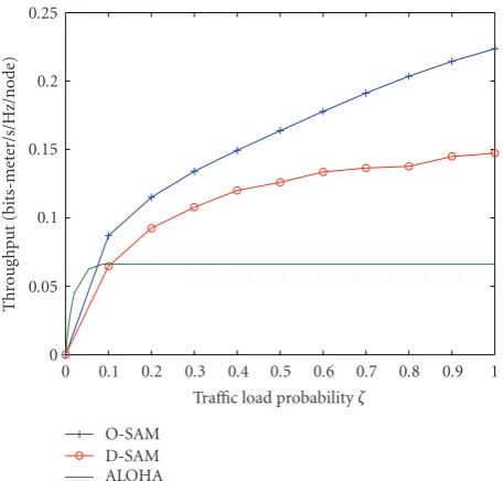
O-SAM D-SAM ALOHA

Figure 6: Throughput comparison of O-SAM, D-SAM, and ALOHA. We usedρ=1, SNR=40 dB, square topology, and SISO channels.

Figure 5shows the throughput of O-SAM versus SNR

and the traffic load probabilityζ. For each pair of SNR and

ζ, the throughput was maximized overξ (the target SINR) andθ(the channel gain threshold). The square topology as shown in Figure 2 was used. The Gaussian SISO channels were considered. This figure is to highlight the fact that the network throughput is saturated to a constant when SNR is large. In the sequel, we will choose SNR=10log₁₀(P/σ2₎₌ 40 dB unless otherwise specified.

Figure 6compares the throughput of O-SAM, D-SAM,

and ALOHA versus the traffic load probabilityζ. For eachζ, the throughput of O-SAM was maximized over bothξ and

θ, and the throughput of D-SAM was maximized overξand

R(the cooperative range). The square topology as shown in

Figure 2and the Gaussian SISO channels were considered.

0 0.02 0.04 0.06 0.08 0.1 0.12 Tra_ffic load probabilityζ

0 0.01 0.02 0.03 0.04 0.05 0.06 0.07

Thr

o

ug

hput

(bits-met

er/s/Hz/node)

1-hop 2-hop 3-hop

ζ=0.01, throughput=0.032

ζ=0.008, throughput=0.023

ζ=0.004, throughput=0.02

Figure 7: Throughput of ALOHA with different transmission ranges: 1-hop, 2-hop, and 3-hop ranges. We usedρ = 1, square topology, and SISO channels. The transmission power for each of the three cases is adjusted so that the SNR (excluding interference) at every receiver is 40 dB.

We see that as long asζ > 10%, both O-SAM and D-SAM yield higher throughput than ALOHA. In other words, only when the traffic load is low, does ALOHA yield a higher throughput. Also note that the transmission probability of ALOHA is optimized for eachζ. But the spacing for O-SAM and the cooperative radius for D-SAM are optimized only for ζ = 1. If those parameters are optimized for each ζ, the throughput curves for O-SAM and D-SAM would be higher forζ < 1. As expected, the throughput of D-SAM is lower than that of O-SAM. This is because the concurrent cochannel transmissions for D-SAM are not as ideal as those for O-SAM. This figure shows that the throughput of D-SAM is about two thirds of that of O-D-SAM in the full load condition.

Figure 7illustrates the throughput of ALOHA for 1-hop,

2-hop, and 3-hop distance transmissions. Note that bits-meter/s/Hz/node is a distance-weighted throughput unit. By 2-hop distance transmission, for example, we mean that the transmission distance between the transmitter and the receiver equals two times the shortest distance between two adjacent nodes. For each of the three cases, we adjusted the transmission power P such that the SNR of the received signal is kept at 40 dB. This means that the transmission power used for 2-hop distance transmission is 2α _times

higher than that for 1-hop distance transmission, and the transmission power used for 3-hop distance transmission is 3α _{times higher than that for 1-hop distance transmission.}

The same square topology as shown in Figure 2 and the Gaussian fading SISO channels were considered. For each

0 0.02 0.04 0.06 0.08 0.1 0.12 Traffic load probabilityζ

0 0.5 1 1.5 2 2.5 3

Ratio

o

f

m

ultihop

thr

o

ug

hput

to

sing

le-hop

thr

o

ug

hput

Throughput ratio of 2-hop over 1-hop Throughput ratio of 3-hop over 1-hop

Figure8: Ratios of throughput: 2-hop range over 1-hop range, and 3-hop rang over 1-hop range. All conditions are the same as for

Figure 7.

of 1-hop distance transmission. In order for 3-hop distance transmission to be better than 2-hop distance transmission, the traffic load probabilityζneeds to be less than 0.4%.

InFigure 8, we show the ratio of the “2-hop distance”

throughput over the “1-hop distance” throughput and the ratio of the “3-hop distance” throughput over the “1-hop distance” throughput. These ratios are lower than one unless the traffic load probabilityζis very small. Whenζapproaches zero, the two ratios become two and three, respectively.

Figures7and8suggest that for peer-to-peer networks, the shortest distance transmission is the most efficient in both spectrum and energy unless the traffic load is extremely low.

Figure 9 compares the throughput of O-SAM and

D-SAM for each of SISO, SIMO, and MIMO cases. For O-D-SAM, the throughput was maximized overξ andθ. For D-SAM, the throughput was maximized over ξ andR. The square network was considered. This figure illustrates that multiple antennas can significantly improve the network throughput.

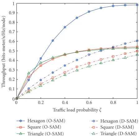
Figure 10compares the throughput of O-SAM and

D-SAM for each of the three topologies: square, triangle, and hexagon. A useful observation is that O-SAM with the hexagonal network has a much higher throughput than all other situations. It is also useful to note here that the optimal subnet partition of the hexagonal network for O-SAM as shown in (2) is identical to that for C-SAM as shown in [14]. Hence, for the hexagonal topology, the throughput gain due to the opportunistic transmitter selection is not compromised by any change of subnet partition. This is not the case for the other two topologies. Although the throughput of SAM is not as high as that of O-SAM, D-SAM works with any topology.

Figure 11illustrates the ξ-optimized throughput of

D-SAM versus the cooperative range R. It is interesting to

0 0.1 0.2 0.3 0.4 0.5 0.6 0.7 0.8 0.9 1 Tra_ffic load probabilityζ

0 0.1 0.2 0.3 0.4 0.5 0.6 0.7

Thr

o

ug

hput

(bits-met

er/s/Hz/node)

MIMO (O-SAM) SIMO (O-SAM) SISO (O-SAM)

MIMO (D-SAM) SIMO (D-SAM) SISO (D-SAM) Figure 9: Throughput of O-SAM and D-SAM for SISO, SIMO, and MIMO channels. We usedρ = 1, SNR =40 dB, and square topology.

0 0.2 0.4 0.6 0.8 1

Traffic load probabilityζ

0 0.1 0.2 0.3 0.4 0.5 0.6 0.7 0.8 0.9 1

Thr

o

ug

hput

(bits-met

er/s/Hz/node)

Hexagon (O-SAM) Square (O-SAM) Triangle (O-SAM)

Hexagon (D-SAM) Square (D-SAM) Triangle (D-SAM) Figure 10: Throughput of O-SAM and D-SAM for different network topologies. We usedρ=1, SNR=40 dB, and 4×4 MIMO channels.

observe that for all three regular topologies, the optimal cooperative rangeR∗ satisfiesda ≤ R∗ < db. Here,da is

the shortest distance between two adjacent nodes, anddbis

the shortest distance between two nodes that are two hops apart. Clearly, whenR < da, the throughput for the regular

topologies should be zero. We also see that for the regular topologies, the throughput in the interval da ≤ R < db

0 1 2 3 4 5 Cooperative rangeR

0 0.05 0.1 0.15 0.2 0.25

Thr

o

ug

hput

(bits-met

er/s/Hz/node)

Random topology Square topology

Triangle topology Hexagon topology Figure11: Throughput of D-SAM versus the cooperative rangeR. We usedρ=1,ζ=1, SNR=40 dB, and SISO channels.

−10 −5 0 5 10

x −10

−8

−6

−4

−2 0 2 4 6 8 10

y

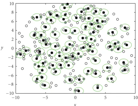
Figure12: A snapshot of subnet partition of a random network by D-SAM withR =0.8. The black nodes are the receivers, and the grey nodes are the transmitters. We usedρ =1 andζ =1. Each circle shown has the radius 0.8.

and not perceivable from this figure. Underda≤R< db, the

corresponding optimal target SINR isξ∗≈4. Givenρ = 1, we haveda = 1 anddb =

√

2da = 1.41

for square;da =

2/√3 =1.07 anddb =

√

3da =1.85 for

triangle; andda=

4/(3√3)=0.877 anddb=

√

3da=1.52

for hexagonal [14]. We will restrictdaanddbto be defined as

above only for the regular topologies.

As observed in our simulation, this optimal condition

da ≤ R∗ < db also holds for α = 3. This observation

interestingly supports the two-hop rule adopted in MSH-DSCH of IEEE 802.16. But the correspondingξ∗ decreases as the path loss exponentαdecreases. We found thatξ∗ is somewhere between 1.5 and 2 whenα = 3. Note that the

spectral efficiency of each packet is governed by the value of

ξ, that is,Rξ =log2(1 +ξ).

Figure 11also shows that forR< da, the throughput of

the random topologies is nonzero, and furthermore it peaks at R = 0.8. It is important to note that the throughput underR< dais not very meaningful. This is because when

R< da, the distance between many adjacent nodes is larger

thanRso that there is no direct link between them. In fact, underR = 0.8, many nodes are not even connected with others, which is illustrated inFigure 12. In such a case, the expression defined in (33) is only a very loose upper bound on the network throughput.

The detailed insights from each simulation example have been presented above. Our overall observations are summarized in the next section.

7. Conclusion

We have presented a further development of synchronous array method (SAM) as a medium access control scheme for stationary ad hoc wireless networks. We have focused on intranetwork throughput enhancement for a large network where any node can be a source node or a destination node. We have used the distance-weighted throughput measure: bits-meter/s/Hz/node. We have presented and evaluated two SAM-based schemes: O-SAM and D-SAM. These two schemes require different levels of centralization and coop-eration within the network.

With O-SAM, the subnet partition within each time frame needs to be predetermined. Provided that the channel coherence time is sufficiently long, local channel estimation is feasible which allows opportunistic exploitation of channel gains within each subnet. The exchange of local information (other than large data packets) can be done via ALOHA-based protocols. In order to induce variations of channel gains, multiple antennas (and a transmit beam vector randomly selected for each frame) can be used at each node. The throughput of O-SAM has been shown to be much higher than that of D-SAM.

With D-SAM, the subnet partition within each time frame is decided by the network locally and dynamically as governed by the cooperative radius (which is smaller than the eavesdropping radius and the carrier sense radius). For networks of sufficiently long channel coherence time, the spectral overhead for exchanges of control packets can be affordable or even negligible compared to the exchanges of data packets. In this case, the network throughput is primarily affected by the subnet partition in each time frame. The cooperative radius R has a major effect on the size of each subnet and hence the network throughput. For networks of regular topologies and full traffic load, the optimal value of R has been shown to be anywhere betweendaanddbwheredais the shortest distance between

two adjacent nodes anddb is the shortest distance between

two nodes that are two hops apart. This result interestingly supports the two-hop rule adopted in MSH-DSCH in IEEE 802.16.