SILC: SPRITE Input Language with C(++)

(1)

S



: S



Input Language with C(

++

)

Master’s Thesis

by

Philip Hölzenspies

Committee: dr. ir. Gerard Smit

ir. Michèl Rosien dr. ir. Jan Kuper prof. dr. ir. Thijs Krol

Cover art by Erik Hagreis

(2)

(3)

Preface

Programming paradigms and compiler techniques have been one of my specific inter-ests for quite a while now, so when Gerard Smit offered me this assignment, it imme-diately felt like it was going to be a lot of fun. “Back then” I was a big fan of_++and was very enthusiastic about the opportunity to study it closer and try and design new models of compilation for it. I say “back then,” because these past few months of re-search have brought surprise after surprise with respect to the behavior of the language. Not all of them nice.

However, the process of researching itself was very enjoyable. Very much so, be-cause of the feisty arguments with Michèl Rosien—in which I was always much too formal—and sparring at the whiteboard with Jan Kuper—where I was never formal enough. I thank them both for these many hours very well spent. Gerard Smit offered me this assignment and for that alone I am grateful, but more so, he stayed calm when I stressed out about deadlines and such. Thijs Krol gave me a real eye-opener halfway into my research, when he completely scattered and rearranged my semantic under-standing of , which eventually helped me a lot. After all, is his work and the

thought that I completely understood all levels of abstraction after reading a concise summarizing paper left me sadly mistaken. Working with the people in my committee was all in all a highly enjoyable and educational experience.

Outside of the committee there are too many people I would like to thank to do that here, so I will simply say I am grateful for all the love I receive daily from friends and family. However, two people have helped in such exceptional ways that they do need to be mentioned explicitly. Erik Hagreis has put a lot of the time he did not have into the design of the cover of this thesis. The result is something to be seen. Likewise, Mark Westmijze has sacrificed a lot of his time to create a presentable demo for me. I must say, his demo has turned out to be quite stunning.

I hope this thesis is useful and reading it will be enjoyable. Writing it certainly has been.

Philip Hölzenspies April 2005

(4)

(5)

List of Figures

2.1 S_example graphs . . . 5

2.2 Examples of common templates . . . 7

2.3 Template for the second and third clause of the additive-expression grammar rule . . . 7

2.4 Transformational design process . . . 9

2.5 Arbitrary labeling function block . . . 10

2.6 Abstraction function block . . . 11

2.7 Example of pattern-based transformations . . . 11

2.8 Structural transformation function block . . . 12

2.9 Operational transformation function block . . . 12

2.10 Hierarchical transformation function block . . . 13

3.1 Dependence between pointers a and b, hard to decide . . . . 16

3.2 Constant propagation in pointer arithmetic . . . 17

3.3 Memory in terms of the pointers to it . . . 17

3.4 Memory in terms of autonomous identities . . . 18

3.5 Symbol table capable operations . . . 21

3.6 Scoping operations adapted to comply with the symbol table model . 22 3.7 High complexity due to the added @-operation . . . 23

3.8 Initial graph and the graph after first transformations . . . 25

3.9 Intermediate transformation results . . . 27

3.10 Final result after transformations . . . 28

4.1 Selection in the linear and block models . . . 32

4.2 Control flow when jumping backwards out of the current scope . . . . 41

4.3 First two steps on the way to a jump model . . . 42

4.4 Last two steps on the way to a jump model . . . 43

4.5 Possible transformation problem . . . 44

4.6 Proof-by-transformation 1 . . . 47

4.9 Block model resulting from transformation . . . 50

5.1 Primitive operations . . . 54

5.2 Jump testing and activation . . . 55

5.3 Landing and jump-safe storage. . . 56

5.4 Shorthands for jumping into and outof scopes . . . 56

5.5 Search operations for scope recursion . . . 57

6.1 Annotation enabling transformation . . . 60

(8)

(9)

1

Introduction

The S_{} Input Language (_) was designed to enable transformational design in

 implementations of electronics. It gives a graphical view of the control- and

data flow through the entire design, because it is itself a Control- and Data Flow Graph (CDFG), or actually a hypergraph. To allow a designer to get a clear overview, it allows for hierarchical abstractions that hide complexity, but still guarantee correctness.

The assignment for this thesis was to extend with types and operations that

would allow the mapping of a greater subset of (++) to it. This need arose from the

observation that designs are often implemented first as a runnable specification. For this purpose_++is used quite often. Moreover, applications in software sometimes need reimplementation in hardware, because they fail to meet (increased) performance criteria. Both of these cases call for an automated translation, because the manual methods often used are error prone and time consuming.

The ‘++’ is parenthesized, because objects and other equally complex extensions ++introduces overare not (yet) included in the supported subset. However,

mix-ture of statements and declarations is, which will be shown to have quite significant implications for the modeling extensions required. Moreover, would there turn out to be conflicts between_[8] and _++[5] then the_++standard was chosen to be the modeling goal.

There have already been some attempts at extending, but they have not yet been

completely successful. Considering that these attempts provided the most important basis for this thesis. A concise description of these extension attempts was drawn up as an internal report by Thijs Krol and Bert-Steffen Visser. Since this report is not available outside of the Embedded Systems group of the University of Twente and the work presented here relies so heavily on it, it has been included as an appendix (see appendix A).

Because of the limited time available for this assignment, a subset of the uncovered language features was chosen. Therefor, the extensions presented here are restricted to pointers and jumps. These two language features were deemed ‘most missed’ and also occur in many (if not most) other imperative languages.

The structure of this thesis is as follows: As it turned out the terms used in the

(10)

(11)

2

The Process

This chapter deals with the process of translation. The conventional way of compiling

++is described briefly in section 2.1. A very brief and informal introduction to

is given section 2.2 (a much more extensive explanation can be found in appendix A). Transformational design is introduced next (2.3) and the consequences for compilation are discussed. Section 2.4 shows how these consequences have been incorporated in the work process used when working with. Finally, the process of transforming

and the nature of transformations is laid out in section 2.5.

2.1

Compiling

++

directly

Commonly, programs are said to have definitions at compile- and run-time. The pro-grammer/designer must be familiar with these concepts in order to deliver proper work. The vast majority of compilers work in some sort of continuous mode and allow for very little (if any) interaction. They are programs themselves that take program code as input, process it and deliver their output. This output can be machine executable code for whatever platform, byte-code for some sort of evaluator or some sort of file used by machines to produce hardware.

Of course, every such output requires its own compiler, because many of these dif-ferent types of output require highly specialized processing (if any level of optimization is desired). There are many compiler suites (e.g. the GNU Compiler Collection) that group different front- and backends and unify the intermediate data structures and pro-cessors. However, all these compilers traditionally work in a batch oriented fashion. Any unrecoverable error (i.e. by the compiler itself) will result in a termination of the compilation process and incomplete output, or none at all.

Real errors should only occur on erroneous input, but failed optimization attempts just result in the original (unoptimized) code they were fed. These optimizations are commonly algorithm based (as opposed to artificially intelligence based) meaning that many are either NP-complete or will not recognize all optimizable structures.

All compilation parameters and hints a designer can give with respect to these

(12)

mizations have to be chosen offline, i.e. before feeding the program to the compiler. It is always possible to change the hints and parameter values and to recompile a program when the original values result in an unsatisfactory compilation.

2.2

S



Sstands for SInput Language and was designed by Thijs Krol et al as an

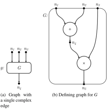
in-termediate format for High Level Synthesis. It needed to have the expressive power and interpretation ease to be applicable to Transformational Design (see section 2.3). S_is based on the notion of hypergraphs. In a hypergraph, a hyperedge connects one set of nodes to another—as opposed to a single node to another—defining (in the case of _) a relation between all the nodes it connects. Actually, nodes are points in the hypergraph that receive a valuation and the hyperedges define relations between these valuations of nodes. For brevity, hyperedges and -graphs are often referred to as edges and graphs, since ‘normal’ graphs are never relevant to this text.

As a rather simple example, consider the graph depicted in figure 2.1a. Nodes, drawn as small circles1_{, are connected by hyperedges. Hyperedges are drawn as boxes}

with arrows to and from nodes. The nodes with arrows to a hyperedge are referred to as the hyperedge’s input nodes and the nodes pointed to by the arrows from a hy-peredge are considered its output nodes. Furthermore, note that the hyhy-peredges are labeled with two labels. The one on the outside (g in the example) is the name of this specific hyperedge and the one in the box (G in the example) is the name of the hyper-edge’s definition. A definition can be given in terms of either another graph, in which case the hyperedge is referred to as complex, or a primitive function, in which case the hyperedge is considered primitive. Primitive hyperedges can be considered to be defining themselves. As a convention, primitive hyperedges are often drawn as (large) circles or ellipses. Nodes are also labeled with their names, but note that both node and edge names are only a way to reference a specific node or edge, i.e. a name is not intrinsically part of the node or edge it refers to.

The hyperedge (often simply referred to as ‘edge’) in the example is complex and, as such, there must be a definition in terms of another graph for this edge. It is de-picted in figure 2.1b. The graph’s name is shown similar to how names of edges are depicted. It turns out G is a graph that has two primitive edges (‘+’ and a ‘×’). Possible definitions for these edges are:

+ : V(i1)+V(i2)=V(o1) × : V(i1)·V(i2)=V(o1)

Where inrefers to the nth input node and omto the mthoutput node. TheVfunction maps nodes to their values and as such these definitions (and the edges that reference them in the graph) define relations on valuations of nodes. Note that these operations happen to be commutative and thus explicit naming of the in- and output nodes is not very relevant. When it is, a graph is usually shown with only the primitive edge and its in- and output nodes, naming the nodes. When it is unclear to what input a node is connected, the arrow connecting it may be labeled with the name of the input. The same holds for outputs. Note that the scope of these names is limited to the edge that

1_In

(13)

Sec. 2.3 Transformational Design 5

(a) Graph with a single complex edge

(b) Defining graph for G

Figure 2.1: Sexample graphs

requires them, i.e. the fact that the output of graph G is named n5 does not conflict

with the fact that the edge g gives its output to node n42.

A more formal and thorough description ofis available in appendix A.

2.3

Transformational Design

The idea that all designer supplied compiler directives are given before actual com-pilation takes place means the designer must be very aware of the capabilities of the compiler and must be familiar with the compilation process. It is possible the designer misses a lot of characteristics of a given program, simply because sometimes relations seem highly complex, when they are not. Moreover, parts of a program might seem very expensive (in terms of execution time) prior to optimization, but might be reduced to something very cheap. This is usually discovered during profiling, but it seems de-sirable to have such information before producing the final output to avoid the need for recompilations.

Moreover, in the context of hardware/software co-design the strict division between compile-time and run-time forces early choices with respect to the separation of hard-and software. By introducing a new hard-and interactive phase in the process of compilation,

transform-time, many of these choices can be made at a later stage when more

infor-mation is available. S_was developed as an intermediate representation—initially for high level synthesis [4,9,10]—for operation during transform-time. It gives a graphical representation of the program being compiled and should thus provide a more intuitive perspective on the functionality of the program to the designer. Another strength of_ is that it can be mapped to a wide variety of different target languages or other outputs. This means that e.g. the choice which parts of a program to implement in hardware can be postponed to a point where it is known what parts really are computationally intensive.

2_{Actually, all names are prefixed by their instantiating environment, so the n}

5of the definition is called

(14)

This transform-time—which is essential in transformational design—can be seen as explicit and interactive compilation. A source language is compiled to the represen-tation used (_). Next, transformations that are proven to leave the external behavior unchanged are performed as per the instructions of the designer [4]. After the designer performs all the transformations he or she deems required, the complete_-graph can be output to a certain output format, or parts can be selected one by one and be out-putted much the same way.

Scan be translated to a multitude of output languages. As said before, it was

primarily intended for high level synthesis and was thus designed to translate from and to languages such as VHDL. It can be argued thatis itself a functional

program-ming language and thus translations to and from other functional languages are very intuitive.

A relatively new application for transformational design involves translating run-nable specifications directly to implementations. It is common practice to first de-liver such a runnable specification to a client to test the interpretation of the design requirements and specifications. Currently, this is often done manually, which is time-consuming and error-prone, so automatic ways of translation are desirable. The basic use case of this application involves translating_++programs to, e.g. VHDL. A close inspection ofshows that it has insufficient notion of ‘state’ to really be able to

trans-late imperative languages to it. With the extensions described in this thesis () it is

now possible to map from and to imperative languages.

Considering the above, it seems worth exploring whether it is possible to adapt

in such a way that it will facilitate translation to and from other languages. In the

most optimistic view, it may even be possible to useas a universal translator. The

extensions to_in_will be restricted to the imperative languages.

2.4

Compiling

++

through



S_ stands for ‘S_{} Input Language (_) with C(₊₊)-extensions’ and it adds an extended notion of state to_. This notion of state will be treated extensively in the following chapters, but a brief introduction is useful here. The state is modeled simply as a very specific type of data, with its own primitives. These primitives basically read and write data3_{from and to addresses in the statespace. The statespace is the collection}

of all possible states, but the term statespace is also used loosely to indicate all states occurring in the program. In++every statement potentially (and presumably) alters

the state implying that (at least initially) the flow through the program is indicated by the changes in the statespace.

For the ‘correctness by construction’ criterion4[4, 10] to be applicable, the initial input of the transform-time interaction must be correct. This means the translation from_++to_must be guaranteed to be correct. To obtain a verifiable translation, the rules of translation should relate as closely as possible to the_++grammar [8]. By using template instantiation with a separate template for every grammar rule, the correctness becomes testable on a per-rule basis.

3_{Since evaluation does not have to be completed for data to be data, they actually read and write}

sub-graphs.

4_{Correctness by construction states that given correct input, any sequence of proven transformations (i.e.}

(15)

Sec. 2.4 Compiling++through 7

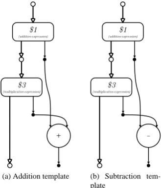
(a) Template for the addi-tive-expression grammar rule

(b) Template for the multiplicative-expression grammar rule

Figure 2.2: Examples of common templates

(a) Addition template (b) Subtraction tem-plate

Figure 2.3: Template for the second and third clause of the additive-expression gram-mar rule

As an example of this mechanism consider the following segment of the++

gram-mar [5, 5.7/1]:

additive-expression: multiplicative-expression

additive-expression + multiplicative-expression additive-expression - multiplicative-expression

The complete template for the grammar rule for an additive expression is depicted in figure 2.2a. In the simplest case, an additive expression is just a multiplicative ex-pression. If this is the case, the inputs of the additive expression template can just be connected to the inputs of the multiplicative expression template (fig. 2.2b). The $n notation is taken from bison’s [2] denotation of the semantic value of the nth _symbol

of the relevant clause; the first rule only has one symbol, so $1 denotes the result of parsing the multiplicative expression.

(16)

Having said that _graphs can simply be seen as functional programs (2.3) and that transformations preserve external behavior5_{, transformations are in essence o}_ffl_ine

evaluation. The problem is, of course, that the complete evaluation can rarely occur at transform-time6_{, so not all run-time information is available yet. Leaving the unknown}

as is, it still often is possible to transform the known parts of the program. Transforma-tions should thus abstract away from the unknown.

An observation is required with respect to what is and what is not unknown. Any program is in itself incomplete if part of its functionality is unknown, so what is allowed to be unknown is restricted to (input)variables. These are modeled either as inputs into the graph, or as unknown constant edges7 [10]. In the first case, no special implica-tions arise, but in the second case it is possible to abstract away from this oblivion by quantifying over all possible (and contextually legal) constant edges.

The following concepts are hereby introduced:

• Let N be a set of nodes. An ordered hyperedge e on N consists of a (possibly empty) setιof input nodes, and a (non-empty) set o of output nodes, i.e.:

e = hι,oi.

Bothιand o are supposed to be ordered. For brevity, the term edge will be used instead of ordered hyperedge. E will commonly be used to denote a set of edges.

If the setιis empty, e is called a constant edge.

• A template t consists of a set of nodes N and a set of hyper edges E on N.

t = hN,Ei

An alternative term for template is hyper graph.

A set of templates is indicated by T.

• Let L be a set of labels. A labeling function f is a function of type E→L, i.e. f

assigns labels to hyper edges. The function f may be partial, i.e. not all edges in a template need to be labeled.

Labeled, non-constant edges are often referred to as (_-)operators.

• A labeled graph C is a 3-tuple

C = hN,E,fi

wherehN,Eiis a template, and f a (possibly partial) labeling function of E.

The templatehN,Eiwill be called the underlying template of the labeled graph

C.

• Let t=hN,Eibe a template, and f,f0_{two labeling functions of E. Let}_ε_⊆_{E be} a set of edges of t such that both f and f0_{are total on}_ε.

Two labeled graphshN,E,fiandhN,E,f0_i_are_ε_{-equivalent (or}_ε_{-isomorphic) if}

f and f0_{assign the same labels to all edges in}_{ε. More formally:}

hN,E,fi_εhN,E,f0i ⇔ f ε=f0ε

whererestricts the functions f,f0_{to the set}_ε.

5_{It is still possible for a designer to make changes to a program in this phase and thus to apply behavior}

altering transformations, but this is an explicit design choice and should not occur automatically

(17)

Sec. 2.4 Compiling++through 9

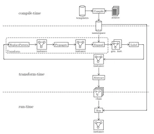
Figure 2.4: Transformational design process

• A graph class is the set of all labeled graphs with the same underlying tem-plate, that areε-isomorphic for a given setε. A graph class will be denoted by

hN,E,f, εi, where f is a representative of the set of all ε-isomorphic labeling functions on E.

Often, we will simply speak of class instead of graph class.

• A labeled graph G in a graph classhN,E,f, εiis an instance of that class, if the labeling function fGof G is total on E and injective onδ=E\ε. Remember that fGε=f ε.

The graph instance G will be denoted ashN,E,f, δi. Note, that the difference in notation between a graph class and a graph instance only consists of the symbols εandδ. In the following text these different symbols (and accented variants like δ0_{) will be used to indicate whether a class or an instance is being discussed.}

In practical terms, the quantification over (constant) edges mentioned above comes down to quantification over all labelings the edge can have. The vast majority of labels is known after compilation, because many elements in a program are in one way or an-other constant (operators, functions, hard coded values, etc). In terms of the definitions given above: a class’ set of edges with fixed labelingsεwill include the majority of the class’ complete set of edges E.

Templates are instantiated during compilation of the source language. The result is a set of (named) graph classes, i.e. the namespace. The labelings of all edges not inε require run-time input, so they will not be available at transform-time. By choosing a

unique random value for these unknown labels, it is possible to calculate relationships

(18)

hN,E,f, δ, ηi //_Label //hN,E,f0_{, δ}0_i

Figure 2.5: Arbitrary labeling function block

values are simply placeholders and do not have any semantic value for the final run-time program, but at least they are guaranteed to be chosen from the graph class. Basically, during transformation any labeling function f0_{may be used as long as it preserves the} ε-isomorphism with the representative labeling function in the namespace and a track record is kept to indicate what edges have been labeled randomly (δ).

These random labels are retracted by abstraction to deliver a graph class that can be instantiated at run-time to get the ‘real’ labelings. Running a program is now reduced to choosing a specific instance of the graph class. Hence when run, a graph is chosen from the class with labeling function g and of course inputs—if required—are given by means of a valuation functionVof the input nodes. The entire process—from source to execution—is depicted in figure 2.4.

2.5

Transformations

In the diagram in figure 2.4 the complete intelligence of transformation is split up into three categories: structural, operational and hierarchical. These transformation categories and the transformations required8 _{for the guarantee of consistency will be}

explained briefly in this section to gain some sort of intuition of the transformation process.

2.5.1

Labeling

The labeling function block (fig. 2.5) appoints trivial, but unique labels to unlabeled edges. It takes as an argument what is loosely called a ‘generic graph instance’, because it is less defined than a graph instance, but more defined than a graph class. It is actually a graph instance with some edges that have not been dummy labeled yet. This means it has an extra set of edgesη⊆E that still require labeling. Thus all significantly labeled

edges in E are E\(δ∪η).

Labeling does not change the structure of the graph itself, i.e.hN,Eiis unchanged, but it chooses a new labeling function in such a way that all chosen and fixed labelings from the previous labeling remain and new labelings are chosen for the edges inη. Hence

f (E\η) = f0(E\η)

δ0 ₌ _δ_∪_η

Note that this means that all edges inδretain the labeling assigned to them by f under

f0_{. The labeling should guarantee that f}0_δ0_{is absolutely injective.}

2.5.2

Abstraction

The labels introduced at transform-time have been used to observe equality, but have no run-time significance. Before running a program, the assumptions made for offline

(19)

Sec. 2.5 Transformations 11

hN,E,f, δi

Abstract

hN,E,f, εi

Figure 2.6: Abstraction function block

(a) Pattern to match (b) Result of transfor-mation

Figure 2.7: Example of pattern-based transformations

evaluation should thus be retracted, i.e. the dummy labels assigned to those edges that were not significantly labeled in the graph class should be ‘removed’. This happens by abstraction from the instance resulting from transformation to a class.

Note that abstraction—as depicted in fig. 2.6—may very well leave the labeling function intact, because in the definition of a graph class, f is a representative label-ing function for theε-equivalence. Retracting the dummy labeling comes down to reversing the indication from which edges are labeled randomly (δ) to which edges are labeled significantly (ε):

ε = E\δ

2.5.3

Structural transformations: pattern replacement

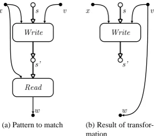
The category of structural transformations concerns mostly pattern replacements, i.e. the replacement of parts of a graph, based on the structure of those parts. Patterns can be defined to describe replaceable structures in a graph. Consider as an example the case that a value vis assigned to variable xin the state and directly after, the same variable is read (asw), than this may be described as a pattern (fig. 2.7a) that can replaced with the behavioral equivalent which still write in the state, but that just copies the value fromvtowdirectly (fig. 2.7b).

(20)

hN,E,f, δi //ReplacePattern //hN0_,_E0_,_f0_{, δ}0_i

Figure 2.8: Structural transformation function block

hN,E,f, δ, ηi //Propagate //hN,E0_,_f0_{, δ}0_i

Figure 2.9: Operational transformation function block

Equality between input values is of course relevant (from the example above, the

address inputs were compared to see they both received x), but in the graph context, equality follows from coming from the same input node. Two inputs can very well be equal when coming from different nodes, but if so, further transformations will—in most cases—unify these different nodes.

Looking at the structural transformation function block (fig. 2.8) a few assertions can be made: both nodes and edges may be destroyed or introduced, so there is no general constraint that can be given on the relations between N and N0and between E and E0. What can be stated is that any edges that remain in the output have unchanged labelings, i.e.

f (E∩E0) = f0(E∩E0) which implies that

δ0 _⊆ _δ

2.5.4

Operational transformations: propagation

Referential transparency is the property of operators and functions in general that guar-antees that constant arguments imply constant results. All operations inare

refer-entially transparent, since the complete state can be an argument of an operation. This observation makes available transformations that take into account knowledge of the definition of operators. When an instance contains operators with exclusively constant inputs, it can be replaced by a set of constant edges; one for each of its outputs.

The function block for this type of transformations is shown in figure 2.9. The same assertion as made for structural transformations holds with respect to the labeling functions, so

f (E∩E0) = f0(E∩E0)

Another important assertion that holds for this category (since it only involves replacing operations with constants for their outputs) is that there will be no introduction of new nodes, hence

N0 ⊆ N

2.5.5

Hierarchical transformations: expansion

(21)

Sec. 2.5 Transformations 13

hNc,Ec,fc, εi

hNi,Ei,fi, δi //Expand //hN0,E0,f0, δ, ηi

Figure 2.10: Hierarchical transformation function block

be a very useful tool, but the automated transformer will only look at relatively small localities and has little to gain from hiding. The semantics of both types of hierarchical transformations are described very clearly in [10, section 2.2], especially the renaming of nodes and edges to unique new names with the exception of in- and output nodes. Only expansion will be treated, but hiding should follow intuitively from the process description given here and the semantics.

Without a complete definition, a homomorphism [1, section 1.4.1]φis used to re-name nodes (φ0 : N → N0) and edges (φ1 : E → E0) conforming to the semantical

definition of expansion9_{. With this homomorphism, consider the function block}

de-picted in figure 2.10. The arguments of the expansion function are the graph instance in which an expansion is necessary and the graph class that defines the edge that is to be expanded. The function results in a generic graph instance (as described in 2.5.1).

Given the definition of a relational image

fS = {f (s)|s∈S}

the following assertions hold (where e is the edge being expanded):

N0 = Ni∪φ0Nc E0 = (Ei\e)∪φ1Ec

f0 = fi∪(λhd,ri.hφ1(d),ri)fc η = φ1Ec\ε

In other words:

• The resulting set of nodes is the set of nodes from the instance expanded with the appropriately renamed nodes from the class being expanded (instantiated).

• The resulting set of edges is the set of edges from the instance expanded with the appropriately renamed edges from the class being expanded.

• The resulting labeling function is the labeling function from the instance ex-panded with the labeling function from the class, where the latter’s domain is renamed according to the renaming of nodes.

• The set of edges that require (dummy) labeling after this transformation is the set of appropriately renamed edges from the class not significantly labeled.

9_Hence,_ϕ

1renames all edges in the graph being expanded such that all their names are unique. Nodes

are renamed byϕ0in such a way that all input and output nodes are given the names of the nodes to which

(22)

Summary

Transformational design is based on ‘correctness by con-struction’, which can only be accomplished by provable translations from the source language to the first instance that will be transformed. To accomplish this, the translation from

++tois based on template instantiation with a

one-to-one correspondence of templates and grammar rules. A new phase—transform-time—in the process is neces-sary to accommodate transformational design in which the designer interacts with a transformation tool to decide what transformations are to be performed.

The program representation of—a hypergraph—is in

fact a functional program. Transformations can therefor be considered offline evaluation of said functional program.

(23)

3

Pointers

In this chapter, some problems arising from the use of pointers are described and solu-tions to deal with these problems are proposed (3.1 through 3.3). These solusolu-tions will be shown to introduce new problems themselves and thus the chapter progressively de-scribes (by iterative solving and examining the solution) the way to the final solution presented in chapter 5. The final section (3.4) a sizable example is given to illustrate the findings of this chapter.

3.1

Problem: Equality and loss of origin

Modeling pointers implicitly by their symbolic name, like any other variable, hides the context of the pointer in the implicit context. When pointers are offset from their base position, the expression itself is required (in its entirety) to determine the referenced location in memory. This means that widespread interdependence requires propaga-tion of a potentially large subgraph through the graph to bring these interdependencies closer together, which becomes very hard when trying to transform it over a possibly infinite recursion.

Consider the example graph shown in figure 3.1 in which it is already determined that the state space does not change in X. For a very complex graph X, the relation between pointer b and address d can not be seen on a local scale, thus, to determine interdependence between pointers a and b, the transformation tool needs to track the full evaluation path of both pointers and see if these paths intertwine somewhere. There should be some way to propagate the constant of the dependence, no matter what the offset evaluates to or depends on, i.e. to partially propagate the eventual value of b.

Even a transformation that should be relatively simple becomes rather complex when using symbolic names as models for pointers. Propagating constants that are added to a pointer along the way turns tricky when the constants are not grouped, but added directly to the pointer. Figure 3.2a shows two constants being added to a pointer

a. In order to perform constant propagation, the transformation of exchanging 3 and a is required first so as to obtain an edge exclusively connected to constant inputs, to

(24)

Figure 3.1: Dependence between pointers a and b, hard to decide

propagate said edge to a constant (fig. 3.2b).

Another problem arising from symbolic representation of pointers is the loss of

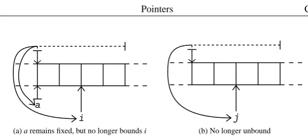
origin. When memory is allocated dynamically, it is not bound to a constant name, but

rather its location is assigned to a pointer. Code snippet 3.1 illustrates the problem. The declaration of a also leads to its allocation and provides a fixed name for the memory reserved at that instance. Pointer j is assigned the address of an otherwise unnamed piece of memory. When i is incremented, the memory it points to still has its point of origin modeled by a, but when j is incremented, there is no means to point to the beginning of the original array.

Code snippet 3.1 Loss of origin

int a [4] , *i = a ,

*j = new int [4]; ... X ...

i ++; ... Y ... j ++;

The problem here is that it is now impossible to use the model for bounds and leak checking1. It is probably possible to check the bounds of i, as it is formulated in relation to a, which is fixed (fig. 3.3a). However, to resolve how many times j could be decremented after its incrementation (fig. 3.3b), the entire evaluation hidden away in

X and Y must be evaluated, which can—needless to say—become very complex.

1_{This might not necessarily be required of the model, but if the ability to perform these checks is available}

(25)

Sec. 3.1 Problem: Equality and loss of origin 17

(a) Unfortunate ordering (b) Optimized result

Figure 3.2: Constant propagation in pointer arithmetic

(a) Bound pointer (b) Afloat in “mid-memory”

Figure 3.3: Memory in terms of the pointers to it

3.1.1

Solution

Pointers require a representation within the model to allow for constant propagation, but it is important to note that this propagation only occurs through a limited arithmetic. Basically, pointers can be assigned, added to or subtracted from. Furthermore, observe that any variable name is in effect a pointer to the actual variable, albeit that it is

dereferenced at compile-time.

Concretely, two requirements have to be met:

• Origin reference: Any address must carry in its representation a reference to the beginning of the block of memory it points into. The representation should not limit the model to specific architectures, so the relation to physical addresses should be abstracted away from.

• Constant propagation: Pointer arithmetic should be propagable as much as pos-sible, meaning that at least every operation with constant arguments should be propagable to a new constant.

These requirements are met by modeling pointers as tuples of a reference to the allocation of the memory pointed into and an offset in terms of the smallest addressable entity2_{. This gives memory allocations an autonomous identity that does not vary with}

transactions on named variables. In the example of code snippet 3.1, using this new

2_{On most stack machines, this would be byte-level, but when transforming to synthesis, this could very}

(26)

(a) a remains fixed, but no longer bounds i (b) No longer unbound

Figure 3.4: Memory in terms of autonomous identities

model simply reformulates the boundaries of a and i and gives a proper formulation of

j (fig. 3.4).

By changing the modeling of a pointer, the model for the state space changes as well, because the symbolic names are no longer connected to locations in memory. Hence, there must be some sort of symbol table, which has locality and should thus be modeled in the state space. Informally, this leads to the following definitions:

address = (allocation index, offset) state space = ({(symbol, address)}

| {z }

symbol table

, {(address, data)}

| {z }

heap

)

3.1.2

Observations

These new “systematic addresses” are globally unique and can not be overwritten. As a direct consequence they are scope independent (as is the case with ‘real life’ memory). The symbol table as specified above would only be capable of modeling scoping if it was treated as an ordered set, where the first occurrence of a symbol is the symbol in the ‘current’ scope [3].

3.1.3

Consequences

With the new definition for the state space, pointer arithmetic allows for constant propa-gation explicitly by observing that there can not be any arithmetic function that projects one pointer onto another if they are not related to the same allocation (i.e. point into the same block of memory). Formally:

∀(x,p),(y,q) :address|x_,y•

@f : (address"address)•f (x,p)=(y,q)

The expression depicted in fig. 3.2a can now be easily propagated, because

a + 5 + 3 = (aalloc, aoffset) + 5 + 3 = (aalloc, aoffset + 5) + 3 = (aalloc, aoffset + 8)

Subtraction can intuitively be defined similarly (with the restraint that the offset remains positive). Subtractions of two pointers should subtract their offsets, but only when both pointers point into the same block of memory (otherwise the semantic value of the expression is void).

a - 5 = (aalloc, aoffset - 5) iff aoffset >= 5

(27)

Sec. 3.1 Problem: Equality and loss of origin 19

Multiplication and division on pointers are not defined in_++, so—observing arith-metic is limited to addition and subtraction—the assumption that aritharith-metic can be performed directly on the offset is valid. Consider snippet 3.2 as an illustration of in-valid arithmetic on_++-pointers, because of possible rounding errors and overflow in multiplication and division.

Code snippet 3.2 Undefined behavior in pointer arithmetic

int a , *p = &a; a = ( int ) p; a *= 2; a /= 2;

p = ( int *) a; // is a ==& a? probably not ! a = *p;

3.1.4

Calibrated pointer arithmetic

In order to truly model++’s real+operation, some form of typing is required.

Ob-serve the code equivalence depicted in snippet 3.3. For 32-bit architectures the sizeof-function applied to an integer (or the keywordint) would return 4, so adding this to a pointer shifts it for the width of one integer value. The incrementation of the int-pointer implicitly calls3asizeof(int)and actually adds the result of this implicit call to the address represented by the pointer, instead of just incrementing the address in an untyped manner.

Code snippet 3.3 Implicit sizing in pointer arithmetic

int a [10] , *p; p = a; p ++;                  ≡                 

int a [10]; byte *p; p = a;

p += sizeof ( int );

Typing should be used to align the data, i.e. to ‘calibrate’ pointer arithmetic. How-ever, now that there are types, it becomes unclear whether the offset should be formu-lated in terms of the type of the pointer (I), or in terms of the smallest addressable entity (II) of the architecture. In (I), the physical equivalent of(alloc id, offset)would then still require alignment and thus comes down to

physical((alloc id,offset)) = valueof(alloc id) + offset ·

sizeof(typeof(alloc id))

and the addition and subtraction operators are defined as follows:

a + x = (aalloc, aoffset + x)

a - x = (aalloc, aoffset - x) iff aoffset == x

a - b = aoffset - boffset iff aalloc == balloc && aoffset >= boffset

This method also requires an observation with respect to pointer casts. When cast-ing from type*ato*bthe offset of the pointer has to be recalibrated, i.e.

(28)

cast(*a, *b, (alloc id, offset)) = (alloc id, jsizeof(a)_sizeof(b)·offsetk) For (II), the calibration is in the operations, which are slightly more complex:

a + x = (aalloc, aoffset + x · sizeof(typeof(a))) a - x = (aalloc, aoffset - x · sizeof(typeof(a))) iff

aoffset >= x · sizeof(typeof(a))

a - b = (aoffset - boffset) · sizeof(typeof(a)) iff aalloc == balloc

Consequently, the physical equivalent of(alloc id, offset)and casting are now a lot more transparent.

physical((alloc id,offset)) = valueof(alloc id) + offset cast(*a, *b, (alloc id, offset)) = (alloc id, offset)

Code snippet 3.4 Differently typed pointers into the same block of memory int i = 0,

*p = &i;

char *q = ( char *) p; ... p ... q ...

The most significant difference between these two methods becomes apparent when considering the constraints these models impose on the model of the heap c.q. the operations on it. When an array is a chain of cells, where these cells have the width required to store a single array element, the (I) method is by far the most intuitive, but when pointers are cast, the arrangement of the memory they point to should change as well. This leads to problems when something like snippet 3.4 occurs. Here bothpand q(andi, obviously) are used to address the same block of memory, but have different types. Alternatively, the operations on the heap could transform these type-dependant offsets to type-independent addresses and then perform their original function.

Code snippet 3.5 Out-of-phase pointers to the same block of memory

int i [10] , *p = i;

char *q = ( char *) p; q ++;

p = ( int *) q;

Besides the esthetic problems these solutions pose, (I) simply fails to model ‘out-of-phase’ pointers. Code snippet 3.5 illustrates the problem. Afterqis assigned the address stored inp, it is used to transposepby the width of achar, but still pointing to segments of the width ofints. Note thatistill points to the original location andqcan shift to any part of the memory block. This situation can not be described by (I), hence (II) will be used to model pointers.

3.2

Problem: symbol table and scoping

(29)

Sec. 3.2 Problem: symbol table and scoping 21

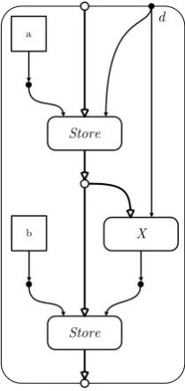
(a) Lookup (b) SymStore (c) SymFetch

Figure 3.5: Symbol table capable operations

The model given earlier works for a single scope, but becomes unpredictable when a nested scope overwrites a symbol.

3.2.1

Solution

Because symbol table and heap are now disconnected, though, it is possible to imple-ment a scoping model in the symbol table and leave the heap as is.

state space = ({(symbol, [(type, address)]

| {z }

scoping

)}

| {z }

symbol table

, {(address, data)}

| {z }

heap

)

This is sufficient to model scope by observing that the topmost entry of the list of type/address-pairs models the definition in the ‘current’ scope [3]. Pointer casts from

*ato*bare now transformations on the state space, albeit very simple transformations because the type-independent heap needs no transformations:

ssin = ({...,(x,[(a, ...),...]),...},{...})

⇓

ssout = ({...,(x,[(b, ...),...]),...},{...})

3.2.2

Consequences

A very significant consequence (ignored earlier) that can no longer be avoided is the explicit need for primitive graph operations to perform state space transactions. Espe-cially when dereferencing pointers, which requires an initial_{}to obtain the address followed by a_{}to obtain the data stored at said address. This implies that these

’s have different input types (symbolic name for the first and address for the

sec-ond), which is not possible. Therefor, the definition of a lookup operation having an input for a symbolic name (sn) is required (fig. 3.5a).

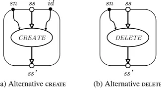
In order to prevent an explosion of complexity of the graph (and of the transforma-tions thereon), the definition of pseudo-primitive operatransforma-tions (SymStoreandSymFetch, figs 3.5b and 3.5c) provides some containment. However, the_{}and_{} opera-tions change (fig. 3.6) in their external typing (there is no sensible definition of a_{} on an address as opposed to on a symbol), and thus correspond only to theSymStore

(30)

(a) Alternative (b) Alternative

Figure 3.6: Scoping operations adapted to comply with the symbol table model

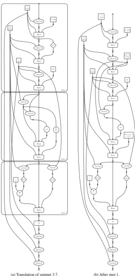
As an illustration of just how much complexity increases, consider the translation of Codesniplet 3.6 into the graph depicted in figure 3.7.

Code snippet 3.6 Simple example of added complexity when using @

int a = 0, *p = &a; *p ++;

3.2.3

Observations

Besides the added complexity of the graph itself, the transformations suffer from added complexity as well. The level of locality is decreased because of the distinction be-tween the symbolic and the concrete representation of variables. In order to establish whether or not adjacent Store and_{}operations are related their inputs can no longer be compared directly. The @-operation that results in the address given to the input of theStoreneeds to be in the locality being considered to be able to determine (in)dependence.

Furthermore, it is worth noting that the @-operation is a compile-time ‘opera-tion’ and does not correspond to any run-time action or state change. Explicit @-operations never simplify or expand the capabilities of the transformations, because of their compile-time application (as opposed to the run-time relevance of transfor-mation). Even more so, symbols themselves are inherently compile-time and have no meaningful representation at run-time (aside from debugging, of course). Therefor, if the graph is to model run-time behavior, it should only include symbolic names as an

assistance for recognition by the designer, not as a semantic element.

Scoping was already implicitly modeled in the graph by the occurrence of the_

-andoperations. Having said that symbols do not exist at run-time, but only

actual addresses are used, there is no need to model scoping in the state space. Besides the fact that transformations simply do not require this information to be explicitly available in the state space—because of their operation on edges in the graph—the fi-nal mapping of graphs to whatever target does not require any such explicit modeling either.

(31)

Sec. 3.3 Problem: No home for types 23

Figure 3.7: High complexity due to the added @-operation

Actually, if the model is to cleanly represent run-time behavior, the symbol table has no place at all in the state space.

3.3

Problem: No home for types

(32)

3.3.1

Solution

Types are, essentially, only required when alignment in the heap is relevant and thus they are only necessary when dealing with pointers, not when dealing with data itself, because data—in the graph—carries its type implicitly in its width. Pointers should thus carry a type and, since pointers are themselves data and thus carry their own type as any other data, the type carried should be that of what is pointed to.

This implies that any fully qualified address carries the type of what it addresses. This might seem counter-intuitive, but in fact, normally the runtime fetches are also ‘width aware’.

3.4

Pointer-model in action

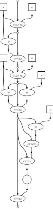
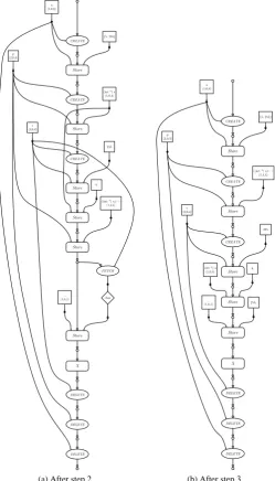
To give an overview of the changes to the model discussed in this chapter, this section will give a more sizable example. Consider code snippet 3.7, which contains some very precarious pointer tricks. For this example, it is assumed that the smallest addressable data unit for the target architecture is a byte. The translation of the code is shown in figure 3.8a.

Code snippet 3.7 Typed arithmetic on pointers

{

int a [2] = {1 , 255} , *p = a , c = 255; (* p ++)++;

*((( char *) p) + 2) += ( char ) c; ... X ...

}

Step 1

The very first_{}in the block corresponding to line 2 of the code can be transformed over theStoreand_{}ofcand can than be deleted, because it now immediately follows aStoreon the same address. When deleting a_{}like this, its output should be connected to the data input of the correspondingStore. Looking at said input it should be observed that the(int *)cast of the original array pointerais a constant operation on a constant input and can thus be propagated. Since integers have a width of four bytes, the type field of the pointer after the cast should be 4, making the complete pointerh1,0,4i.

One of the edges taking the resulting pointer as input is the pointer incrementation. This operator ‘increments’ the pointer, not by simply adding 1 as is the case with integers and other incrementable types, but by the type argument, i.e.

h1,0+1·4,4i=h1,4,4i

These transformations result in the graph shown in figure 3.8b.

Step 2

(33)

Sec. 3.4 Pointer-model in action 25

(a) Translation of snippet 3.7. (b) After step 1.

(34)

Storeand_{}ofp, because even though an address with allocation id 1 is stored on p,pitself has allocation id 2 and thus the two operation are not interdependent. This

brings the_{}operation being transformed immediately next to the corresponding

Store. Even though the Store of a (h1,0,8i) and the_{} of (int *) a(h1,0,4i) operate on different sizes, it is possible to replace the_{}with a constant based on the data input of theStore. The resulting constant 5 can also be propagated through the connected increment operator.

Anotherthat can be transformed out of the graph is the one performed on

p, which is an immediate successor of aStore on the same address. It can thus be replaced by a direct connection to the data input of theStore. This results in a nicely propagable subgraph of exclusively constant edges. The cast to a character pointer results inh1,4,2iand the following addition of constant 2 results (fig. 3.9a) in

h1,4+2·1,1i=h1,6,2i

Step 3

The last remaining_{}in the graph (ofc) can be transformed upwards, similar to the ones before. This connects the constant 255 to the cast operator. This is a propagable constant operation and can thus be replaced by a constant. Since data casts only affect the width of the data, a subscript is added4_{to indicate the width in bytes.}

Because all_{}operations have been transformed out of the graph at this point, the secondStoreofpcan be transformed upward across the operations on(int *) a andc(as neither have allocation id 2). After this transformation theStoreis the imme-diate successor of another store onpand thus overwrites the latter’s effects. The first can thus be discarded, resulting in 3.9b.

Step 4

The remaining transformations are those that carry the two bottom Storeoperations upward to their corresponding . They are both operations on allocation id 1,

which is that ofa. They can both be transformed without any difficulty to the initial

Store of a. Since alignment of arrays is fixed in_++, theStore onh1,0,4i can be

propagated and combined with the initialStore, resulting in a single operation. The secondStore being transformed upward can not be unified, because no assumptions have been made so far about the architecture with respect to endianess and thus the alignment of characters in the space of an integer is unknown.

The final result is shown in figure 3.10. If at this point the designer can indicate the target architecture is big-endian the doubleStoreoperation at the top of the graph can be unified to a single store, storing{6,65535}. The translation back to++of the graph

is shown in snippet 3.8 together with the result if the designer would indeed perform the final transformation assuming big-endianness of the target architecture.

4_{Subscripting the width of a constant is an ad hoc choice made here and di}_ff_{erent implementations may}

(35)

(a) After step 2. (b) After step 3.

(36)

Figure 3.10: Final result after transformations

Code snippet 3.8 Typed arithmetic on pointers

{

int a [2] = {6 , 255}; *((( char *) a) + 2) =

( char ) 255; int *p = a [1] , c = 255; ... X ...

}                                be ⇒                        {

int a [2] = {6 , 65535} , *p = a [1] , c = 255; ... X ...

(37)

Summary

Pointers should be transformable through pointer arithmetic, but should not cross the boundaries of the memory blocks into which they point. To guarantee pointers can not traverse into coincidentally neighboring blocks of memory, all allo-cations are modeled as strictly unique, using an allocation identifier that is guaranteed to have a one-to-one relationship with the block of memory resulting from the allocation.

Under the uniqueness constraint, all transformations are legal. They are modeled using transformations on the offset from the beginning of the allocated block of memory. These offsets are expressed in terms of the smallest addressable en-tity of the architecture (or target language) and not in terms of elements of the associated type.

Types are relevant at run-time only for data alignment and are thus only needed when having to extract data from the heap. Therefor, addresses carry the type (width) of the data pointed to and data has no need for explicit typing, since it implicitly describes its type by having an unambiguous width.

(38)

(39)

4

Jumps

This chapter discusses the differences in jump scenarios (4.1) and all these different scenarios are reduced to the generalized form. Next the machine behavior of jumps is analyzed (4.2) and an attempt is made to identify the theoretical minimum of informa-tion required to model jumps. Something needs to be said about scoping in the context of jumps (4.3), before finally giving a general model for all classes of jumps (4.4).

4.1

Selected notes on types of jumps

Essentially jumping constructs can be categorized as ‘structural’ and ‘unconditional’. A construct is considered structural, when it delimits the full block of code that the jump crosses. Selection and iteration statements constitute the structural jump con-structs in_++. All these structural constructs are mapable to unconditional constructs and—in particular—to the ‘most unconditional’ jump, i.e. thegoto. These categories of jumps will be treated separately in the next few pages.

4.1.1

Selection statements

Selection statements redirect the flow of control through code block alternatives, i.e. segments of code are either selected for execution or passed by. The selection state-ments in++are

if condition statement

else

statement

and

switch (condition)

statement

(40)

(a) Linear machine model (b) (Code)block model

Figure 4.1: Selection in the linear and block models

These statements have possible side effects in their conditions, so these should first be allowed to alter the statespace before any block is executed.

It actually depends on the model chosen whether these selection statements consti-tute jumps or not. In the linear machine model, they do (fig. 4.1a), but in a (code)block model (i.e._) there really is a notion of selection (fig. 4.1b), hence the name.

Selection statements add a single level of scoping. Anything declared in the

con-dition is in scope in the nested statement(s), but out of scope outside of the construct.

Implications of this observation will be treated in section 4.3.

It deserves mentioning thatswitch-statements usecase-labels only as jump targets. These labels do not alter the flow of control in any way [5, 6.4.2] and the target is chosen beforehand. This is why case labels have to be compile-time constants and can not alter the statespace.

Code snippet 4.1 Case label illustration

int i = 2; switch (i) {

case 1: ... A ... break ; default : ... B ... break ; case 2:

... C ... }

(41)

Sec. 4.1 Selected notes on types of jumps 33

difference, because the target is chosen at the top. This means that the compiler would have to gather information from the nested statement to find out what jump labels are actually available, as opposed to the per-keyword translation that can be performed on anif-statement. This is made even more complex by the fact that case labels are not constrained to the current scope, they may well cause jumps into deeper scopes.

4.1.2

Iteration statements

The_++-standard [5, 6.5/1] specifies three iteration statements1_{, viz.}

while ( condition )

statement

do

statement

while ( expression ) ;

for ( for-init-statement conditionopt ; expressionopt ) statement

Code snippet 4.2 Invariant of afor-loop as awhile-loop

for (I C; E) S          ≡                                      { I while (C) { S E; } }

The last two of these have very well known invariants in terms of the first (and vice versa). Afor-loop can be rewritten to awhile-loop as shown in snippet 4.2 (note that the braces are significant for scoping). Snippet 4.3 shows the reverse mapping.

Code snippet 4.3 Invariant of awhile-loop as afor-loop

while (C) S          ≡         

for (; C ;) S

Thewhile-statement (and thus any iteration statement) is simply a very special case of recursion [15]. In_++, however, there are some specifics with respect to scoping. Iteration statements—like selection statements—add one level of scoping, but it is im-portant to note that every iteration jumps to a point before the entry of said scope. The consequences of this will be discussed in section 4.3.

(42)

4.1.3

Unconditional jumps

There are a few different types of unconditional jumps. They are break ;

continue ;

return [ e x p r e s s i o n ]; goto identifier ;

Thebreak-statement is used to jump out of iteration statements andswitch-statements (there would be no use to use it to jump out ofif-statements, because it is usually used within anif-statement inside an iteration orswitch-statement. The continue-statement can only occur inside iteration continue-statements and it jumps to the ‘end of the current iteration’.

Both of these statements can be rewritten togoto-statements, albeit that some label-generation (and guaranteed uniqueness) is required. In a sense, one could say that an iteration statement binds all free occurrences ofbreak- andcontinue-statements (see [1], 6.2.2) and that these jump statements may not occur globally unbound.

Because of this binding requirement, it could be argued thatgoto-statements are ‘more unconditional,’ i.e. their application is also unconditional as opposed to that of continues enbreaks. The only restriction on agotois that it has to jump to a label

inside the current function.

Only thereturn-statement is not strictly rewritable to agoto-statement, because it explicitly exists the current function scope. However, modelwise a function can be defined as having a__return_value__variable by default of the same type as the return type of the function itself. It would then ‘return’ (i.e. result in, evaluate to) whatever value is stored in said variable whenever it comes to its end.

All these jumps are unified to theirgotoequivalents in the next section.

4.1.4

Unified jumping

As a matter of fact, all these different types of jumps are unifiable in a single jumping model, using onlygotos and stripped downifs. Basically, the unified jumping model is very closely related to stack machine models. In this modelifs are only allowed to havegotos in their bodies and never have anelse. This closely models the notion of ‘jump if nonzero’ and its antonym when using the!(not) operator.

In the following loose translations conditionsCwill be assumed to have a declara-tion of typeTandC’will be said condition without the declaration2, i.e.

C≡T c = C’

When conditions do not contain such a declaration, their translation can be the same, only with omission of the explicit declarations given below.

A translation of the ‘normalif’ now looks like snippet 4.4. Theswitch-statement is a bit more complex because the alternatives given in the case labels must be gathered in a separate pass by the compiler first. The translation then follows as shown in snippet 4.5. When aswitch-statement does not have adefault-label in its nested statement, goto default;is changed togoto brk;(or thedefault-label is inserted right before thebrk-label. Any free occurrence ofbreak-statements inB0throughBnare substituted bygoto brk;.

2_{It should be understood that multiple declarations are possible in the condition, but for brevity, a single}

(43)

Sec. 4.2 Selected notes on types of jumps 35

Code snippet 4.4 Translation of the ‘normalif’

if (C) S1 else S2                  ≡                                          {

T c = C ’;

if (! c) goto else_part ; S1

goto end_if ; else_part :;

S2 end_if :; }

Code snippet 4.5 Translation of theswitchstatement

switch (C) {

B0 case X1 :

B1 case X2 :

B2 ... default : Bn }                                                    ≡                                                                            {

T c = C ’

if (c == X1 ) goto case_X1 ; if (c == X2 ) goto case_X2 ; ...

goto default ; B0 case_X1 :; B1 case_X2 :; B2 ... default :; Bn } brk :;

Iteration statements can also be rewritten to the unified model. Firstly, thedo-while statement translates directly (snip. 4.6). Similarly, thewhilestatement can be trans-lated (snip. 4.7). Since theforis just an invariant of the while—as discussed before— the translation shown in snippet 4.8 follows intuitively. In this last translation, the nestedwhileshould be translated according to thewhiletranslation shown before.

Similar to theswitch-statement translation, all free occurrences ofbreakare trans-lated togoto brk;and likewise freecontinues are translated togoto continu;. It goes without saying that these labels require some administration to keep them unique, but for legibility they have been kept simple here.

Finally thereturn-statement should be translated to this unified jumping model. The problem that arises, though, is thatgotois defined to jump to a label in the same

(44)

Code snippet 4.6 Translation of thedo-whilestatement

do S while (C );

             ≡                                begin_loop :; { S continu :;

if (C) goto begin_loop ; }

brk :;

Code snippet 4.7 Translation of thewhilestatement

<