Supplementary material to:
A: Supplementary tables and figures
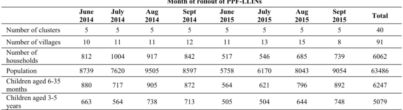
Table A1. Characteristics of study area according to the census.
Month of rollout of PPF-LLINs June
2014
July 2014
Aug 2014
Sept 2014
June 2015
July 2015
Aug 2015
Sept
2015 Total
Number of clusters 5 5 5 5 5 5 5 5 40
Number of villages 10 11 11 12 11 13 15 8 91
Number of
households 812 1004 917 842 517 546 685 739 6062
Population 8739 7620 9505 8597 5758 6170 8043 9054 63486 Children aged 6-35
months 880 717 905 872 564 621 796 892 6247
Children aged 3-5
years 663 564 738 713 505 504 644 748 5079
Table A2. Characteristics of replacement children enrolled into the cohort at the third survey (May 2015).
Month of rollout of PPF-LLINs
Characteristics June 2014 July 2014 Aug 2014 Sept 2014 June 2015 July 2015 Aug 2015 Sept 2015 Total
Children
enrolled, N 73 63 99 84 101 76 84 95 675
Female, N (%) 41/73 (56%) 33/63 (52%) 50/99 (51%) 41/84 (49%) 54/101 (53%) 41/76 (54%) 35/84 (42%) 47/95 (49%) 342/675 (51%) Age (months),
median (IQR) 30 (21,39) 29 (21,43) 30 (18,41) 29 (20,41) 29 (17,40) 29 (19,46) 34 (24,47) 29 (21,40) 29 (20,42) Sleeps under a
mosquito net, N (%)
73/73 (100%) 61/63 (97%) 99/99 (100%) 84/84 (100%) 100/101 (99%) 75/76 (99%) 83/84 (99%) 94/95 (99%) 669/675 (99%)
Took anti-malarials in last 14 days, N (%)
0/73 (0%) 1/63 (2%) 0/99 (0%) 2/84 (2%) 1/101 (1%) 1/76 (1%) 0/84 (0%) 0/95 (0%) 5/675 (1%)
Sick with a fever during previous 48 hours, N (%)
1/73 (1%) 4/63 (6%) 4/99 (4%) 11/84 (13%) 2/101 (2%) 4/76 (5%) 1/84 (1%) 2/95 (2%) 29/675 (4%)
Axillary temperatures (°C), median
(IQR) 36.4 (36.2,36.5) 36.4 (36.2,36.7) 36.3 (36.2,36.7) 36.5 (36.2,36.9) 36.4 (36.2,36.8) 36.4 (36.2,36.8) 36.5 (36.2,36.7) 36.5 (36.2,36.8) 36.4 (36.2,36.7) Positive rapid
diagnostic test, N (%)
1/1 (100%) 3/6 (50%) 3/4 (75%) 7/12 (58%) 3/3 (100%) 4/6 (67%) 0/1 (0%) 3/4 (75%) 24/37 (65%)
Presence of Plasmodium falciparum parasites by microscopy, N (%)
26/73 (36%) 29/62 (47%) 47/98 (48%) 40/83 (48%) 50/99 (51%) 31/71 (44%) 38/83 (46%) 44/95 (46%) 305/664 (46%)
>5000 Plasmodium falciparum parasites per μl, N (%)
6/73 (8%) 9/62 (15%) 7/98 (7%) 15/83 (18%) 19/99 (19%) 12/71 (17%) 5/83 (6%) 13/95 (14%) 86/664 (13%)
Plasmodium falciparum parasite density (per μl), geometric mean (geometric SD) of non-zero
gametocytes, N (%)
Haemoglobin level (g/L), median (IQR)
112.0 (107.0,115.0)
101.0
(94.0,111.0) 103.0 (98.0,111.0) 105.0 (99.0,111.0) 102.0 (96.0,111.0) 103.5 (96.0,111.0) 102.0 (99.0,110.0)
103.0 (100.0,109.0)
104.0 (99.0,111.0) Moderate
anaemia (haemoglobin <80 g/L), N (%)
2/73 (3%) 4/57 (7%) 2/99 (2%) 3/84 (4%) 6/101 (6%) 4/76 (5%) 1/83 (1%) 3/95 (3%) 25/668 (4%)
Severe anaemia (haemoglobin <50 g/L), N (%)
0/73 (0%) 0/63 (0%) 0/99 (0%) 0/84 (0%) 0/101 (0%) 0/76 (0%) 0/84 (0%) 0/95 (0%) 0/668 (0%)
Enlarged spleen (defined as score >0 using Hackett classification), N (%)
6/73 (8%) 1/63 (2%) 0/99 (0%) 1/84 (1%) 3/101 (3%) 3/76 (4%) 7/84 (8%) 0/95 (0%) 21/675 (3%)
Table A3. Incidence of clinical malaria in the cohort: unadjusted and adjusted regression models.
Model adjusted for [1] RR (95% CI) for PPF-LLINsvs. standard LLINs P value for PPF-LLINs vs.standard LLINs P value for adjustmentvariable AIC
Nothing 0·72 (0·66,0·78) <0·001
-Calendar month [2] 0·89 (0·78,1·01) 0·07 <0·001
Calendar month and health facility [2,3] 0·88 (0·77,0·99) 0·04 Health facility: <0·001Month: <0·001 27361
All the following adjusted for calendar month [2], health facility and:
Age (categorised) 0·87 (0·77,0·99) 0·04 <0·001
When joined the cohort (survey 1 or 3) 0·87 (0·77,0·98) 0·03 <0·001 Coverage (whether slept under bed net last night, defined at entry into the
cohort) 0·88 (0·77,0·99) 0·04 0·84
Cluster size, defined by number of children per cluster 0·88 (0·77,0·99) 0·04 0·33 Random effect for village, instead of cluster 0·86 (0·76,0·97) 0·02
-Alterative adjustments for time (all adjusted for health facility):
Year only (2014, 2015), ignoring month 0·95 (0·86,1·05) 0·29 28494
Month only (May, June, …, Dec), ignoring year 0·72 (0·66,0·79) <0·001 27463
Month and year as separate variables (May, June, …, Dec; and 2014, 2015) 0·87 (0·77,0·99) 0·03 27449
Repeating with ONLY months where there are data from both arms (all adjusted for health facility):
Calendar month [2] 0·86 (0·73,1·01) 0·07 16656
Year only (2014, 2015), ignoring month 1·04 (0·88,1·22) 0·69 17220
Month only (May, June, …, Dec), ignoring year) 0·86 (0·74,1·00) 0·05 16654
Month and year as separate variables (May, June, …, Dec; and 2014, 2015) 0·86 (0·73,1·01) 0·07 16656
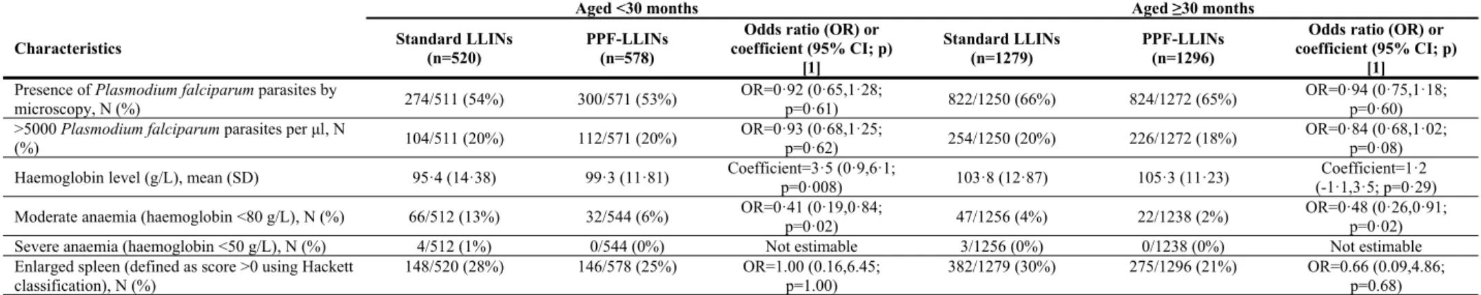
Table A4. Secondary and tertiary endpoints at the second cross-sectional survey, by arm: stratified by aged <30 versus ≥30 months.
Aged <30 months Aged ≥30 months
Characteristics Standard LLINs(n=520) PPF-LLINs(n=578) coefficient (95% CI; p)Odds ratio (OR) or [1]
Standard LLINs (n=1279)
PPF-LLINs (n=1296)
Odds ratio (OR) or coefficient (95% CI; p)
[1]
Presence of Plasmodium falciparum parasites by
microscopy, N (%) 274/511 (54%) 300/571 (53%)
OR=0·92 (0·65,1·28;
p=0·61) 822/1250 (66%) 824/1272 (65%)
OR=0·94 (0·75,1·18; p=0·60) >5000 Plasmodium falciparum parasites per μl, N
(%) 104/511 (20%) 112/571 (20%) OR=0·93 (0·68,1·25;p=0·62) 254/1250 (20%) 226/1272 (18%) OR=0·84 (0·68,1·02;p=0·08) Haemoglobin level (g/L), mean (SD) 95·4 (14·38) 99·3 (11·81) Coefficient=3·5 (0·9,6·1;p=0·008) 103·8 (12·87) 105·3 (11·23) (-1·1,3·5; p=0·29)Coefficient=1·2
Moderate anaemia (haemoglobin <80 g/L), N (%) 66/512 (13%) 32/544 (6%) OR=0·41 (0·19,0·84;p=0·02) 47/1256 (4%) 22/1238 (2%) OR=0·48 (0·26,0·91;p=0·02) Severe anaemia (haemoglobin <50 g/L), N (%) 4/512 (1%) 0/544 (0%) Not estimable 3/1256 (0%) 0/1238 (0%) Not estimable Enlarged spleen (defined as score >0 using Hackett
classification), N (%)
148/520 (28%) 146/578 (25%) OR=1.00 (0.16,6.45; p=1.00)
382/1279 (30%) 275/1296 (21%) OR=0.66 (0.09,4.86; p=0.68)
Analyses stratified by age were pre-specified for haemoglobin levels but not for the other secondary outcomes. Includes cohort and additional children, but excluding children during the month of and month after the introduction of the intervention. [1] Odds ratio or coefficient with 95% confidence interval and p-value for PPF-LLINs versus standard LLINs, using logistic and linear regression models for categorical and continuous variables, respectively, with cluster as a random effect and health facility as a fixed effect.
Table A5. Secondary and tertiary endpoints at the second cross-sectional survey, by arm: stratified by cohort versus additional children.
Cohort children (survey 2) Additional children (survey 2)
Characteristics Standard LLINs(n=887) PPF-LLINs(n=908)
Odds ratio (OR) or coefficient (95% CI; p)
[1]
Standard LLINs (n=912)
PPF-LLINs (n=966)
Odds ratio (OR) or coefficient (95% CI; p)
[1]
Presence of Plasmodium falciparum parasites by
microscopy, N (%) 475/866 (55%) 494/892 (55%)
OR=1·03 (0·80,1·32;
p=0·84) 621/895 (69%) 630/951 (66%)
OR=0·82 (0·64,1·05; p=0·12) >5000 Plasmodium falciparum parasites per μl, N
(%) 146/866 (17%) 150/892 (17%)
OR=1·00 (0·77,1·28;
p=0·98) 212/895 (24%) 188/951 (20%)
OR=0·80 (0·61,·0·96; p=0·02) Haemoglobin level (g/L), mean (SD) 101·7 (13·78) 104·4 (11·78) Coefficient=2·2 (0·0,4·4;p=0·05) 101 (13·9) 103 (11·6) (-1·0,4·0; p=0·23)Coefficient=1·5
Moderate anaemia (haemoglobin <80 g/L), N (%) 50/875 (6%) 25/868 (3%) OR=0·52 (0·30,0·88;p=0·02) 63/893 (7%) 29/914 (3%) OR=0·48 (0·20,1·16;p=0·10) Severe anaemia (haemoglobin <50 g/L), N (%) 3/875 (0%) 0/868 (0%) Not estimable 4/893 (0%) 0/914 (0%) Not estimable Enlarged spleen (defined as score >0 using Hackett
classification), N (%)
248/887 (28%) 208/908 (23%) OR=1.82 (0.17,19.2; p=0.62)
282/912 (31%) 213/966 (22%) OR=0.43 (0.06,3.29; p=0.42)
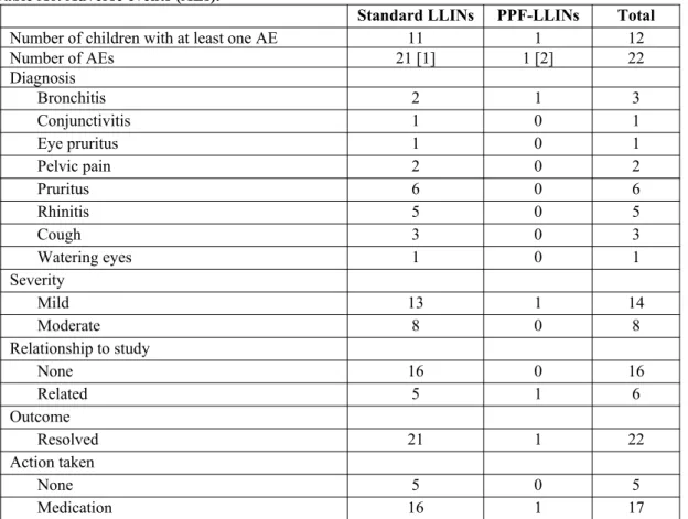
Table A6. Adverse events (AEs).
Standard LLINs PPF-LLINs Total
Number of children with at least one AE 11 1 12
Number of AEs 21 [1] 1 [2] 22
Diagnosis
Bronchitis 2 1 3
Conjunctivitis 1 0 1
Eye pruritus 1 0 1
Pelvic pain 2 0 2
Pruritus 6 0 6
Rhinitis 5 0 5
Cough 3 0 3
Watering eyes 1 0 1
Severity
Mild 13 1 14
Moderate 8 0 8
Relationship to study
None 16 0 16
Related 5 1 6
Outcome
Resolved 21 1 22
Action taken
None 5 0 5
Medication 16 1 17
Presented by arm at time of AE. [1] One child had cough, followed the next day by watering eyes. One child had rhinitis and cough, followed by rhinitis again one month later. One child had pruritus, followed the next day by rhinitis. One child had pruritus on two consecutive days, followed two days later by cough and pelvic pain, followed the next day by rhinitis. One child had bronchitis, followed two days later by conjunctivitis. One child had pruritus twice, approximately two months apart. [2] AE occurred <1 month after rollout of PPF-LLINs.
Table A7. Serious adverse events (SAEs).
Standard LLINs PPF-LLINs Total
Number of children with at least one SAE 9 9 18
Number of SAEs 10 [1] 9 [2] 19
Diagnosis
Severe malaria 6 1 7
Severe malaria and pneumonia 0 1 1
Severe malaria and urinary infection 1 0 1
Severe malaria and skin infection 0 1 1
Uncomplicated malaria and vomiting 1 0 1
Gastro-enteritis and severe dehydration 0 1 1
Pneumonia 1 0 1
No information 1 5 6 [3]
Type of SAE
Died 1 5 6
Hospitalisation 9 4 13
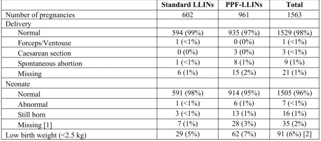
Table A8. Pregnancies.
Standard LLINs PPF-LLINs Total
Number of pregnancies 602 961 1563
Delivery
Normal 594 (99%) 935 (97%) 1529 (98%)
Forceps/Ventouse 1 (<1%) 0 (0%) 1 (<1%)
Caesarean section 0 (0%) 3 (0%) 3 (<1%)
Spontaneous abortion 1 (<1%) 8 (1%) 9 (1%)
Missing 6 (1%) 15 (2%) 21 (1%)
Neonate
Normal 591 (98%) 914 (95%) 1505 (96%)
Abnormal 1 (<1%) 6 (1%) 7 (<1%)
Still born 3 (<1%) 13 (1%) 16 (1%)
Missing [1] 7 (1%) 28 (3%) 35 (2%)
Low birth weight (<2.5 kg) 29 (5%) 62 (7%) 91 (6%) [2]
Presented by arm at time of delivery. [1] Includes those with missing delivery information and spontaneous abortion. [2] Missing for 10 and 46 pregnancies in the standard LLIN and PPF-LLIN groups, respectively (percentages are of non-missing values).
Table A9. Asthma.
Standard LLINs PPF-LLINs
Number of children with asthma [1] 40 15
Score
<15 (asthma not under control) 0 0
15-19 (asthma partially under control) 4 (10%) 3 (20%)
20-25 (asthma under control) 36 (90%) 12 (80%)
For study subjects identified with asthma, we used the asthma control test method to monitor them for the month following the net donation (standard or PPF LLINs) to document any aggravation of symptoms.1 33 children
had data only from the period during which they were in the standard LLIN arm, 8 children had data only from the period during which they were in the PPF-LLIN arm, and 7 children had data from both the period during which they were in the standard LLIN arm and during which they were in the PPF-LLN arm (these children contribute data to both columns). For multiple visits for the same child within one arm of the trial, the mean score was taken. The median number of visits per child was 5.5 and 4 within the standard and PPF-LLN arms, respectively (range 1-8 and 1-7, respectively).
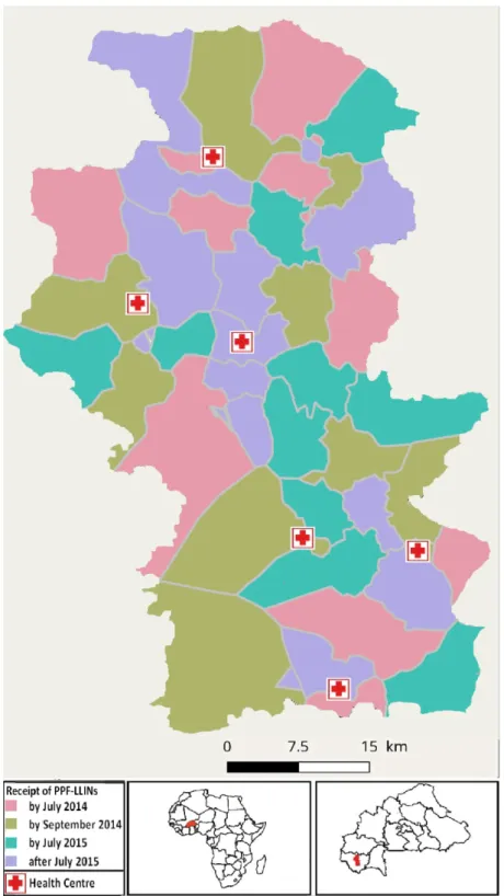
Figure A1. Roll out of the pyriproxyfen and permethrin long-lasting insecticidal nets.
0 200 400 600 800 1,000 1,200 N u m be r of c as es
jun 20 14
jul 20 14 aug 20
14 sep 20
14 oct 20
14 nov 20
14 dec 20
14
may 2 015
jun 20 15
jul 20 15
aug 20 15
sep 20 15
oct 20 15
nov 20 15
dec 20 15 External to study area
0 200 400 600 800 1,000 1,200 N u m be r of c as es
jun 20 14
jul 20 14 aug 20
14 sep 20
14 oct 20
14 nov 20
14 dec 20
14
may 2 015
jun 20 15
jul 20 15
aug 20 15
sep 20 15
oct 20 15
nov 20 15
dec 20 15 Study area
B: Operating characteristics of different parasitaemia cutoffs Introduction
In areas highly endemic for Plasmodium falciparum, many individuals who have no acute symptoms of the disease carry malaria parasites in their blood. The detection of parasites in patients presenting with fever is often used as an operational definition of clinical malaria in epidemiological studies and field trials. In such areas, some patients so diagnosed as clinical malaria are suffering from fevers of non-malaria etiology, but are considered as clinical malaria cases because of incidental parasitaemia. This leads to overestimation of the number of cases, and reduces the specificity of the definition of clinical malaria, leading to a downward bias in estimates of efficacy in comparative field trials.
The specificity of the case-definition can be improved by imposing a requirement for parasite densities in fever patients to exceed a threshold value, before classifying them as clinical malaria (often a cut-off of 5000 parasites/μl, as determined by microscopy is used). Formal statistical analysis of the quantitative relationship between disease incidence and parasite density can be carried out to estimate the operating characteristics of different thresholds.2 This is achieved by comparing the distribution of parasite densities in population surveys,
with that in fever patients. This analysis also provides an estimate of the proportion of the malaria attributable fraction of fevers,
λ
.This document reports the application of this analysis to the data of the pyriproxyfen net trial. The sensitivities, specificities, and attributable fractions were estimated separately for each arm of the trial. The values obtained are used to estimate the bias in effectiveness estimates that would apply if different density thresholds were adopted. The analysis also provides an estimate of effectiveness that avoids these biases by using the attributable fractions to estimate the numbers of clinical malaria episodes in each arm, without the need to classify each individual patient.
Methods
The analytical approach treats the parasite densities for fever patients,
x
1, x
2, … x
n,
as a sample from a mixturewith two components,
θ
(corresponding to negative samples equivalent to control (population survey) samples) andϕ
(corresponding to positive samples with higher values of x than the controls) so that:p
i=
(
1
−
λ
i)
θ
i+
λ
iϕ
i (C1)where:
p
i=
P
(
x ϵ category i
)
;θ
i=
P
(
x ϵ category i
∨
x ϵ θ
)
; ϕ
i=
P
(
x ϵ category i
∨
x ϵ ϕ
)
;
andλ
iis theprobability that a fever case in category i has true malaria etiology (this increases with i Aparasitaemic patients cannot be true malaria cases, so
λ
1=
0
, makingϕ
i, θ
i,
andλ
i identifiable.A latent class model, using the method of Vounatsou et al3 is used to obtain Bayesian estimates of all the
quantities in equation C1 using a Markov chain Monte Carlo algorithm in the package WinBUGS.4 The
WinBUGS code used to fit this model is provided below.
The sensitivities and specificities of different candidate threshold parasite densities can be expressed as
functions of
ϕ
i, θ
i,
andλ
i. For the case definition using the i th parasite density threshold, (corresponding to thelower boundary of the category) these are computed as:
sensitivity
=
∑
j=i
k
ϕ
j, andspecificity
=
1
−
∑
j=i
k
θ
j/
∑
j=i
k
p
jλ
=
∑
i=1
k
λ
iϕ
iUsing the microscopy results from the trial, the effectiveness estimated using each parasite density threshold, is:
E
i=
1
−
n
Cm
I∑
j=i
k
p
i ,Cn
Im
C∑
j=i
k
p
i , Iwhere the subscripts C and I refer to the control and intervention arms respectively, the quantities n and m are the total numbers of patients and surveyed individuals in the corresponding arms, and the sums,
∑
j=i
k
p
i, give the proportions of fever cases satisfying the case definition. This is the conventional estimate of effectiveness (the values ofm
Iandm
C appear in order to scale the corresponding counts of episodes by the person-time-at-risk, assumed to be proportional to the number of survey attendees).The estimate of effectiveness that uses the attributable fractions,
λ
, to estimate the numbers of clinical malaria episodes in each arm without classifying each individual patient is then the adjusted effectiveness estimate:E
=
1
−
n
Cm
Iλ
Cn
Im
Cλ
IResults
The samples used for analysis were grouped into 9 categories of parasite density (Table C1). Table C1: Numbers of samples included in analysis of parasite densities
Lower bound of density
(parasites per µl)
Cross-sectional surveys Fever cases
Control Inter-vention Control Inter-vention
0 2225 3415 324 525
1 486 753 91 104
500 388 636 71 86
1000 499 890 113 120
2500 419 588 115 113
5000 311 515 104 121
10000 279 431 208 270
25000 88 136 293 317
50000 81 91 507 660
Figure C1: Estimates of
θ
i(distribution of parasite densities in non-malaria fever or survey samples) Error bars correspond to 95% credible intervals; vertical lines to a threshold of any parasitaemia by microscopy. The constraints that the ratio of malaria:non-malaria cases increases with parasite density, and that fevers in aparasitaemic (or sub-patent) patients are assumed to be of non-malaria etiology, lead to estimates ofλ
i thatincrease strongly with parasite density around values of around 5000 parasites/μl (Figure C2).
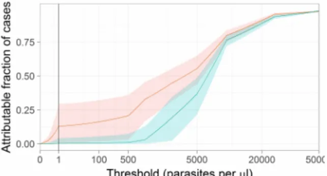
Figure C2: Estimates of the probability cases are malaria attributable,
λ
i , by parasite density. Shaded envelopes correspond to 95% credible intervals; Colours and vertical lines as per Figure C1.The overall estimates of the attributable fractions,
λ
, are 0·609 (95% CI 0·569-0·648) for the control arm, with a slightly lower value of 0·528 (95% CI 0·500-0·556) for the intervention arm.Since values of
λ
i vary considerably with i, the estimated distributions of parasite densities in the malariaattributable fever cases (Figure C3) are very different from those in the surveys.
Figure C3: Estimates of
ϕ
i (distribution of parasite densities in true malaria cases) Colours and lines as per Figure C1.Figure C4: Sensitivity of parasite density thresholds Colours, shading and vertical lines as Figure C2.
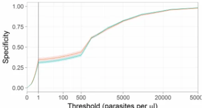
As anticipated, there is a substantial increase in specificity with parasite density, with a threshold value of around 5000 parasites/μl required to achieve a specificity above 80% (Figure C5). This implies that many cases with low parasite densities included in the primary trial analysis are sick because of causes other than clinical malaria.
Figure C5: Specificity of parasite density thresholds Colours, shading and vertical lines as Figure C2.
The extent to which the inclusion of non-malaria fevers biases the estimate of effectiveness is illustrated by the effectiveness estimates made using the different thresholds (Figure C6).
Figure C6. Effectiveness estimates made using different thresholds
Thick black line, unadjusted estimates; red line adjusted estimate; vertical line corresponds to threshold of any parasitaemia by microscopy.
Somewhat contrary to expectations, the effectiveness estimates do not increase with the use of higher (more specific) thresholds. However, the adjusted estimate of effectiveness of 0·295 (95% CI: 0·232-0·351), (obtained by assigning probabilities that fevers are malaria attributable as functions of the parasite density) is higher than the effectiveness estimates obtained by using any fixed cutoff. In particular, the estimate obtained using the threshold of any parasitaemia by microscopy, of 0·236 is 20% lower than the adjusted value. This suggests that there is a considerable downward bias in the primary efficacy measure because of inclusion of non-malaria fevers, but that the fevers with the highest parasite densities were no more likely to be in the control arm than were malaria fevers with lower densities.
Discussion and conclusions
There is no evidence in these data of any important imbalances between the arms in terms of the distributions of parasite densities in infected individuals, and clinical malaria cases in the two arms have similar parasite density distributions.
Winbugs code model latentclass {
for (a in 1:arms) { for (i in 1:2){ z0[a,i]<-(i-1)*0.0001 phi0[a,i]<-theta[a,i]*z0[a,i] } theta[a,1]<-1-St[a] eltheta[a,1]~ dgamma(1.0,1.0) theta[a,2]<-eltheta[a,2]/(1+Sr[a]) eltheta[a,2]~ dgamma(1.0E-2,1.0E-2) for (i in 3:K){
phi0[a,i]<-theta[a,i]*z0[a,i] eltheta[a,i]~ dgamma(1.0E-2,1.0E-2) theta[a,i]<-eltheta[a,i]/(1+Sr[a]) z0[a,i]<-z0[a,i-1]/q[a,i] } Sn[a]<-sum(n[a,]) Sm[a]<-sum(m[a,]) Sr[a]<-sum(eltheta[a,2:K]) St[a]<-sum(theta[a,2:K]) Sp[a]<-sum(p0[a,]) Sphi0[a]<-sum(phi0[a,]) for (i in 1:K){
phi[a,i]<-phi0[a,i]/Sphi0[a] z[a,i]<-z0[a,i]/Sphi0[a] q[a,i]~dunif(0.001,0.999) p0[a,i]<- theta[a,i]*(1-lambda[a])+lambda[a]*phi[a,i] p[a,i]<-p0[a,i]/Sp[a] lami[a,i]<-lambda[a]*phi[a,i]/p0[a,i] }
# Computation of sensitivities and specificities of cutoffs sens[a,1] <- 1.0
spec[a,1] <- 0.0
cum_theta[a,1] <- theta[a,1] cum_phi[a,1] <- phi[a,1] cum_p[a,1] <- p[a,1]
unadj_cases[a,1] <- Sn[a]/Sm[a]
adj_cases[a,1] <- Sn[a]*lambda[a]/Sm[a] for (i in 2:K){
sens[a,i] <- sens[a,i-1]-phi[a,i-1]
cum_theta[a,i] <- cum_theta[a,i-1] + theta[a,i] cum_phi[a,i] <- cum_phi[a,i-1] + phi[a,i] cum_p[a,i] <- p[a,i-1] + p[a,i]
spec[a,i] <- 1 - (1 - cum_theta[a,i-1])/(1 - cum_p[a,i-1]) # Total cases included by threshold,
# scaled by population at risk (via total of m)
# adj_ refers to adjustment for incidental parasitaemia unadj_cases[a,i] <- (1 - cum_p[a,i-1])*Sn[a]/Sm[a] adj_cases[a,i]<-(1-cum_phi[a,i-1])*Sn[a]*lambda[a]/Sm[a] }
m[a,1:K]~ dmulti(theta[a,1:K], Sm[a]) n[a,1:K]~ dmulti(p[a,1:K], Sn[a]) lambda[a]~ dunif(0.00001,0.99999) }
adj_eff [i]<- 1 - adj_cases[2,i]/adj_cases[1,i] }
C: Estimation of EIR
To model the numbers of female A. gambiae collected per trap, we used a negative binomial model, with village cluster as a random effect, and treatment arm, month and health facility as fixed effects. The means by arm were estimated marginally over month and health facility, assuming a random effect of zero. We used a logistic regression model with the same random and fixed effects to model the sporozoite prevalence, and the prevalences by arm were estimated similarly.
For arm
i
=
0
(standard LLINs) andi
=
1
(PPF-LLINS), letHDM
i indicate the household density ofmosquitoes and
SPR
i indicate the sporozoite proportion, estimated as described above. Letn
represent thenumber of days in the transmission season (
n
=
214
). As per the main manuscript, the entomological inoculation rate (EIR) was estimated for each armi
as follows:EIR
i=
HDM
i× SPR
i× n
The ratio of the EIR was determined as
EIR
1/
EIR
0.To estimate 95% confidence intervals, we treated
HDM
i andSPR
i as independent variables and used anasymptotic approximation following Armitage and Berry (1). Let the means of
HDM
i andSPR
i be denotedμ
i1 andμ
i2, respectively, and their variancesσ
i1 andσ
i2, respectively. Then the variances of the product ofHDM
i andSPR
i for each armi
are given by:var
(
HDM
iSPR
i)
=
μ
i21σ
i22+
μ
i22σ
i21+
σ
i21σ
i22We then used a Normal approximation to estimate the confidence intervals for the product
HDM
iSPR
i, and finally multiplied the confidence limits byn
=
214
.For the confidence interval of the ratio
EIR
1/
EIR
0, we used the approximation:var
(
EIR
1/
EIR
0)
=
var
(
EIR
1)
E
(
EIR
0)
2+
E
(
EIR
1)
2
E
(
EIR
0)
4var
(
EIR
0)
D: Insecticide-susceptibility tests. Discriminating Dose Assays
Results of the WHO susceptibility tests performed during the study. Mosquitoes were collected from three health districts in the Cascades region, Burkina Faso. Health districts are specified within brackets. Mosquitoes were collected as larvae in July (Tiefora and Bakaridjan in 2014) or October (Naniagara and Bakaridjan 2015).
2014 2015
Village Replicate Mortality n Replicate Mortality n
Tiefora Centre (Tiefora) 1 2 22 1 0 25
2 4 25 2 1 27
3 6 27 3 0 24
4 1 23 4 0 21
Total 13 97 Total 1 97
% mortality 13.4 % mortality 1.03
Naniagara (Kankounadeni) 1 5 29 1 1 27
2 1 25 2 2 27
3 2 26 3 6 23
4 2 19 4 11 24
Total 10 99 Total 20 101
% mortality 10.1 % mortality 19.8
Bakaridjan (Koflande) 1 7 21 1 4 24
2 9 22 2 3 29
3 3 18 3 6 31
4 1 26 4 4 31
5 7 30 5 6 22
6 3 18
7 2 32
Measurements of intensity of permethrin resistance.
A modified version of the CDC bottles assay was used to estimate the permethrin Lethal
Concentration 50 (LC50), which is the dose that kills 50% of a population for mosquitoes collected
from the three health districts in October 2013. Bottles were coated internally with different concentrations of permethrin (ranging from 5 ppm to 120 ppm) following the procedure described by
CDC5 and the modifications proposed by Bagi et al 6Four groups of approximately 25 three to five
days old female mosquitoes were aspirated into the bottles and exposed for 60 min. Mosquitoes were then transferred to paper cups with 10% sucrose available, and mortality recorded 24h later. In every experiment control bottles impregnated only with the solvent (acetone) were also tested.
The permethrin LC50 ranged from 17.8 ppm in Bakaridjan mosquitoes to 29.7 ppm in Naniagara
mosquitoes (Figure D1). There was a significant difference in the LC50 between Bakaridjan and the
other two sites although the difference between the highest and lowest value was less than 1.7-fold.
The permethrin LC50 for the Kisumu susceptible strain was previously calculated as 0.284 ppm6, and
thus estimates of the resistance ratio of the field populations range from 60.7 to 115.1 fold.
References
1. Armitage P, Berry G. Statistical methods in medical research. Oxford: Blackwell Scientific; 1994. 2. Smith T, Amstrong Schellenberg J, Hayes R. Attributable fraction estimates and case definitions for
malaria in endemic areas. Statistics in Medicine 1994; 13: 439-42.
3. Vounatsou P, Smith T, Smith AFM. Bayesian analysis of two-component mixture distributions applied to estimating malaria attributable fractions. AJ R Stat Soc Ser C Appl Stat 1998; 47: 575-87.
4. Spiegelhalter D, Thomas A, Best N, Lunn D. WinBUGS Version 1.4 Cambridge, England MRC-BSU; 2003.
5. Brogdon W, Chan A. Guideline for evaluating insecticide resistance in vectors using the CDC bottle bioasssay. . Atlanta: CDC, 2010.