FULL TEXT Reason and Data

HEINEMANN SENIOR MATHEMATICS

_)! __

tieinemann Educational Australia

'

r

i

i·

,, ·,,

,·

I

i

(

l

branches and representatives throughout the world. ©J.B. Fitzpatrick and P. L. Galbraith 1990 First published 1990

Reprinted 1991

All rights reserved. No part of this publication may be reproduced, stored in a retrieval system or transmitted in any form by any means whatsoever without the prior permission of the c_opyright owner. Apply in writing to the publishers.

Edited by Scharlaine Cairns, Charlie C. Editorial Pty Ltd Designed by Tom Kurema

Illustrations by Gavin Mount

Keying and preparation of disks by Tricia Randle Typeset in Times Roman by Savage Type Pty Ltd, Brisbane Printed in Singapore by Chong Moh Offset Printing National Library of Australia

Cataloguing-in-publication data: Fitzpatrick, J. B. (John Bernard).

Reasoning and data Includes index. ISBN O 85859 527 3.

l . Mathematics. I. Galbraith, P. (Peter). II. Henry, Bruce. Ill. Title. (Series: Heinemann senior mathematics).

Contents

(Projects and Investigations are identified by

[;J

and

U

respectively.)

Acknowledgements (x)

Preface [xi)

Chapter 1 Statistics 1

1.1

Graphical representation of data 2

(;I

1.2

Limited-over cricket 9

1.3

Continuous and discrete data 10

1.4

Frequency distribution 10

1.5

Histograms 12

1.6

Frequency polygons 14

1. 7

Measures of central tendency 17

1.8

Measurement of dispersion 22

(;I

1.9

Multi-lingual 'Scrabble' 30

Chapter 2 Probability 31

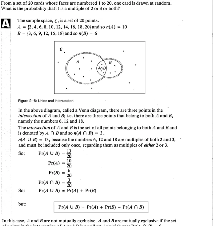
2.1

Complementary events 35

2.2

Life tables (1984) 36

2.3

Finite sample space 40

2.4

Mutually exclusive events 41

2.5

Successive outcomes 45

2.6

Independent events 50

2.7

Conditional probability: a reduced sample space 61

2.8

Baye·s• Theorem 70

Chapter 3 Permutations and combinations 77

3.1

Permutations 78

3.2

The multiplication principle 79

3.3

Mutually exclusive operations: addition principle 81

3.4

Definition of permutation 81

3.5

The symbol npr

83

3;6

Arrangements with restriction� 85

3. 7

Arrangements in a circle 88

3.8

Number of arrangements of n objects

in a row, when they are not all different 89

(v)

3.9

Combinations 92

3.10

The symbol (;) or

93

3.11

Probability associated with permutations and combinations 100

Chapter 4 Binomial distribution

111

4.1

Binomial theorem

112-4.2

Binomial probability distribution 117

4.3

Mean and v�riance of a discrete random variable 127

4.4

Mean and variance of a binomial distribution 129

l];I

4.5

Coin tossing 133

l];I

4.6

Computer simulation of binomial experiments 134

Chapter 5 Other discrete probability distributions

137

5.1

� Hypergeometric distribution: sampling without replacement 138

5.2

Mean and variance of a hypergeometric distribution 143

5.3

Geometric distribution 146

5.4

Poisson distribution 149

5.5

Exponential distribution 157

l];I

5.6

Poisson distribution project 157

5.7

Probability and matrices: Markov chains 159

Chapter 6 Normal distribution

167

6.1

The normal distribution 168

6.2

Standard normal curve 169

6.3

Normal approximation to binomial distribution 179

6.4

Probability limits for a single value of the normal variable 182

6.5

Probability limits for the sample mean of

n

values of the variable 186

6.6

Confidence limits 188

Revision exercises (Chapters 1 to 6)

197

Chapter 7 Problem-solving and investigations 20s

7.1

Problems 206

D

7 .2

Investigations 214

Chapter 8 Related variables

219

8.1

Scatter diagrams 220

8.2

Regression of

yon x

221

8.3

Method of least squares 222

8.4

Bivariate distributions: two regression lines 224

8.5

Correlation 231

8.6

Correlation and causation 237

D

8. 7

Correlation investigation 239

8.8

Non-linear relationships 240

8.9

Time series -245

8.12

Measurement of seasonal variations 253

8.13

Forecasting using single moving average 256

Chapter 9 Non-parametric statistical tests

9.1

Hypothesis testing: stating the hypotheses 264

9.2

The sign test 265

9.3

Significance level 266

9.4

The steps in performing a statistical test 266

9.5

Binomial test of percentiles 267

9.6

Wilcoxon test for two independent samples 270

9. 7

Dealing with ties 272

9.8

Dealing with large samples 272

9.9

Permutation test 273

9.10

Statistical project 277

9.11

; . The Chi-square test 277

9.12

Degrees of freedom, v 279

9.13

x

test for a Poisson distribution 281

9.14

x

test for a normal distribution 282

9.15

x

test for a binomial distribution 284

9.16

Contingency tables 287

(;J

9.17

Newspaper poll 293

9.18

Die-tossing program 293

9.19

Tables 295

Chapter 10 Graphs arid optimisation

297

10.1

Graph theory 298

10.2

Basic definitions and properties 299

10.3

The handshaking lemma 301

10.4

Isomorphic graphs 302

10.5

Cycles and trees 307

10.6

Applications to network problems 308

10. 7

Planar graphs 310

10.8

Eulerian paths 313

10.9

Fleury's Algorithm 316

10.10

Network inspection problems 317

10.11

Shortest path problems 318

10.12

Hamiltonian graphs 320

10.13

The travelling sales representative problem 320

(;J

10.14

Road network 326

D

10.15

Chemical molecules 327

10.16

Digraphs (directed graphs) 328

10.17

Matrix representation 328

10.18-.

:Applications of digraphs 331

(;J

10.19

Graphing projects 339

(vii)

263

Chapter 11 Logic and reasoning

341

11.1

Propositions 342

11.2

Negation, -

p

342

11.3

Set notation 343

11.4

Conjunctionp /\ q

344

11.5

Disjunctionp v q

345

11.6

Conditional statements

p � q

349

11. 7

Converse, inverse and contrapositive 350

11.8

Equivalencep

q

351

11.9

Tautologies 358

11.10

Negation of compound sentences 361

11.11

Validity of arguments 363

11.12

Use of tautologies 366

11.13

Quantifiers 368

Chapter 12 Methods of proof

373

12.1

Mathematical proof 374

12.2

Necessary and sufficient conditions 375

12.3

Proof patterns in mathematics 375

12.4

Indirect proof 378

12.5

Proof by counter-example 379

12.6

Famous proofs from antiquity 381

12. 7

Mathematical induction 384

12.8

Problem solving and investigations 390

D

12.9

Logic investigations 392

(;I

12.10

Logic projects 394

12.11

Finite differences 395

D

12.12

Cheese slicing 398

D

12.13

Pizza party 398

D

12.14

The twelve days of Christmas 398

(;I

12.15

Number patterns 399

Chapter 13 Boolean algebra

401

13.1

Laws of set algebra 403

13.2

Boolean algebra 404

13.3

Principle of Duality 405

13.4

Theorems in Boolean algebra 405

13.5

De Morgan's laws 407

D

13.6

Boolean algebra investigation 409

13.7

Examples of Boolean algebras 410

13.8

Electrical circuits 412

13.9

Simplification of circuits 413

13.10

Boolean functions 415

13.11

Disjunctive form 415

13.12

Conjunctive form 417

13.13

Functions of three variables 417

14.2

Antidifferentiation by parts 427

14.3

Other density functions 429

14.4

Measures of location for probability distributions 438

14.5

The mean (expected value) of

g(X)

444

14.6

Variance and standard deviation 444

Chapter 15 Euclidean geometry (extension)

449

15.1

Assumptions 450

15.2

Angle properties of atriangle 451

15.3

Congruent triangles 456

15.4

Similar triangles 464

15.5

Theorem of Pythagoras 468

15.6

Circle theorems 473

15.7

Cyclic quadrilaterals 478

15.8

Tangents to a circle 482

15.9

Alternate segment 484

15.10

Intersecting chords of a circle 488

15.11

Concurrency theorems 490

Summary

495

Answers

503

Index

531

The authors with to express their thanks to Mr Ted Byrt, formerly of State College Rusden

Campus, for his contribution and helpful suggestions in the area of statistics.

The authors and publisher would like to thank the following individuals and organisations

for their assistance in providing photographs and for their permission to reproduce

copyright material:

Charles Ciurleo, pp. 77 (a, b, c), 137 (b) and 219; D. A. Heffernan, p. 401; The

Herald

&

Weekly Times Ltd,

Melbourne, pp. 77 (d), 263 and 423; Tattersall Sweep Consultation,

pp. 205; Tubemakers of Australia Ltd, p. 167.

Every effort has been made to trace and acknowledge copyright material and the authors

and publisher would welcome any information from people who believe they own copyright

material used in this book.

Reasoning and Data provides a comprehensive coverage of the compulsory sections of the

unit, together with detailed coverage of eight of the content clusters. The book also provides

for study of Reasoning and Data at the extension level, with coverage of the probability,

statistics, and algebra requirements together with two selections (calculus and geometry)

from the additional study areas.

With respect to the work requirements, essential content in the area of probability is

contained within Chapters 2, 4, 5 and 6. The compulsory statistics material is contained in

Chapters 1, 4, 5 and 6. Chapter 1 is an introduction, consolidating aspects of data

representation that will have been studied to varying degrees in past years. The other

chapters systematically introduce discrete and continuous distributions together with their

special features, and related calculations of statistical measures and estimates of parameters.

The logic requirements are provided for within Chapters 2, 10, 12 and 13. Set diagrams are

utilised in probability work (Chapter 2) and also in the chapters on logic and reasoning

(Chapter 11) and Boolean algebra (Chapter 13). The concept and application of proof

appears in the chapters on logic and reasoning (Chapter 11), graphs and optimisation

(Chapter 10), methods of proof (Chapter 12) and Boolean algebra (Chapter 13). 'Graphs

and optimisation' (Chapter 10) contains all the material necessary for the study of

undirected graphs.

The algebra section is well covered. Chapter 3 contains applications of combinations; basic

equation solving and formula manipulation is required regularly throughout almost all

chapters; set algebra is used widely in Chapters 3, 11 and 13; sequences and series are

applied in Chapters 8 and 12, and Chapter 8 also includes work on non-linear relationships.

The companion volumes Space and Number and Change and Approximation contain

additional material that systematically addresses analytical and numerical methods for

solving equations and inequations.

Clusters of content

The following chapters contain material that enables comprehensive coverage of the

nominated clusters.

Combinations

Chapters 3 and 4

Sampling processes

Chapter 4

Probability distributions -

geometric, Poisson and exponential

Chapter 5

Time series analysis and economic statistics

Chapter 8

Correlation and regression

Chapter 8

Non-parametric statistics

Chapter 9

Logic and proof

Chapters 11 and 12

Boolean Algebra

Chapter 13

In addition, substantial amounts of material pertaining to the Clusters (Random sampling,

Estimation and confidence intervals, and Directed graphs) are also included.

For the extension course, Chapters 2, 3, 4 and 6 contain extension material for

probability;

Chapter 6 provides extension material for

statistics;

and Chapter 3 provides extension

material for

algebra.

Within the additional area of study, two options are provided; 'Calculus extension'

(Chapter 14) and 'Euclidean geometry extension' (Chapter 15).

The treatment of the subject matter emphasises coherence so that, where relevant, extension

material appears as a natural development bf the core material. Chapter 7 'Problem solving

and investigations' provides material particularly geared to problem solving, modelling, and

project work.

Features of the presentation include:

• a systematic and thorough introduction to, and consolidation of, content material to

promote concept understanding and facility in skills and standard applications. Numerous

worked examples and sets of exercises are included to this end, including sets of revision

exercises.

• provision of problem-solving examples, modelling situations, investigations and project

material integrated through the chapters, in addition to those provided in Chapter 7.

• integration of the electronic calculator throughout, and provision of computer-based

learning tasks for concept learning, applications and investigation and project work.

Project material is defined in terms of its nature rather than its length. School projects of

varying lengths may be obtained by combining one or more text-based projects. Text-based

Projects

and

Investigations

are frequently presented in a sequential fashion so that

variations between students can be provided for, e.g. not every student may be required to

complete every part of such an activity. A computer application often forms the final section

of a Project I Investigation and can be retained or omitted without otherwise affecting the

structure.

The authors endorse the spirit and intent of the general course structure and its work

requirements.

It is expected that many effective modelling s_ituatfons, investigations and

projects will be designed with the local school environment in mind. This book provides a

supporting base upon which such local emphasis can be built, while at the same time

containing more than sufficient material to meet the work requirements in all areas.

Computer Policy Statement

Throughout this text and its companion volumes there are a number of short programs for

carrying out specific mathematical tasks. Students are also given the opportunity to write

their own programs to help in some of the exercises, applications and models.

It is not the place in a text such as this to teach the elements of computing. These will have

been mastered already by anyone wishing to use a computer productively with this book.

We are aware that there is a degree of debate about programming languages such as BASIC,

LOGO and PASCAL, and each has its supporters. We have chosen to use the BASIC

language, not because it is the best, but because it is the most universally available on the

facilities available to most students. Those who wish to work in another language have the

opportunity to do so, by converting the coding that is provided or by working directly from

the verbal context of the exercises, applications and models.

We do not favour the blind, uncritical use of computer programs in a mathematics course

and have endeavoured at all times to provoke productive thinking in the use of such

programs. This has been done, for example, by encouraging the interpretation of lines of

coding, the amending of programs and the optional use of computers in work dealing with

applications and modelling, where appropriate. In providing coding alone we indicate our

recognition that the matter of flow-charting is one of debate. We have chosen not to make

flow-charting a necessary step in creating programs. The use of flow charts (or not) is,

therefore, at the discretion of the user.

1

Statistics

2 STATISTICS

'Statistics', in a broad sense, deals with scientific methods of collecting, recording and

summarising data from which future trends can be predicted, or which can be used as a

basis for making decisions and drawing valid conclusions.

Government departments use data collected by statisticians to observe trends in such areas

as population growth, urban development and employment, so that provision can be made

for public transport, schools, hospitals, playgrounds, and so on. Can you think of other

uses by government departments of statistical data?

Sporting commentators use statistics to compare the performances of individuals and teams,

for example cricketers' batting and bowling averages.

The school uses statistics in the form of class lists and student subject choices to help

determine the number of teachers needed, classroom allocations, number of desks and

lockers required, and so on. Your teachers are using statistics when they analyse and

interpret your assessment results to determine your progress or to obtain the class average

in various subjects.

Industry and commerce use statistics, for example, to help reduce the number of defective

items produced by machines. If records show that a particular machine is constantly

producing inferior quality articles, management uses this information to decide if the

machine should be repaired or replaced. Can you think of other uses of statistics in industry

and commerce?

1.1 Graphical representation of data

Statistical data are frequently presented in the form of graphs and charts and it is useful

to be able to:

a provide a pictorial representation of the data

b interpret data from a pictorial representation.

Example 1

In 1987, 705 people died on Victorian roads. These people were either drivers, passengers,

pedestrians, motorcyclists (and pillion passengers) or bicyclists as shown in the following

table:

Road user

Drivers

Passengers

Pedestrians

Motorcyclists

Bicyclists

Total

We can illustrate this data by means of:

(i) a column graph

(ii) a bar graph

(iii) a pie chart.

Number killed

Percentage

310

43.9

166

23.6

137

19.5

67

9.4

25

3.6

705

100%

The bar graph, in Figure 1-2, is similar to the column graph, but bars or rectangles of any

width replace the vertical lines of the column graph. The bars are equally spaced and of

the same width. Frequently, in a bar graph, the bars are placed horizontally instead of

vertically.

Number killed

310

166

137

67

25

Figure 1 -1 : Column graph

Figure 1-2: Bar graph

Number killed

310

166

137

25

D

D

I

Pa Pe M B

Pa Pe M B

. The pie chart, in Figure 1-3 shows the number of each type of road user killed expressed

as a proportion or percentage. The steps used in drawing the pie chart are:

a Express the number killed as a percentage.

Drivers: ���

= 43.9%

Passengers:

�i�

= 23 .6%, etc.

b Convert each percentage into its equivalent part of a circle, in degrees.

Drivers: 43.9% of 360

= 158

Passengers: 23.6% of 360

= 85

, etc.

c Draw a circle and, with the aid of a protractor, mark accurately the sector representing

each type of road user.

Figure 1-3: Pie chart

Example 2

The bar graph in Figure 1-4 shows the profit, before and after tax was paid, of a chain store

operating throughout Australia. The information is given in the table below.

Year

1984

1985

1986

1987

1988

Profit before tax in $ million

20

30

40

45

55

Profit after tax in $ million

12

17

25

30

35

The full height of each rectangle in Figure 1-4 represents the profit before tax.

The information given in Example 2 can also be illustrated by means of a

line graph,

as

in Figure 1-5. It should be noted that only the position of the dots represents the

information given. The steepness of the lines joining these dots indicates the degree of

increase or decrease. For exampie, the profit after tax rose more sharply from 1985 to 1986

than in any other year.

Figure 1-4

Figure 1-5

Profit

$ million

t:·:·:·:·I Tax

60

- Profit after tax

50

40

30

20

10

1984 1985 1986 1987 1988

Profit

$ million 60

50

40

30

20

-- Profit before tax

--- Profit after tax

--.. ----

--- ---k

''

---

--10

1984

1985

1986

...

...

--1987

_

...

Exercises 1a

(Most of these questions are based on data supplied by the Australian Bureau of Statistics.)

1 The table on the right shows the

percentage of imports into Victoria

from various countries, and the

exports from Victoria to other

countries, in 1986-87.

Represent the data by means of bar

graphs and make any comments you

consider to be relevant.

Country

USA

Japan

Germany

UK

China

Italy

Hong Kong

Singapore

Other

Imports

Exports

25.7

14.2

19.2

14.6

9.7

4.0

7.2

-6.4

8.8

3.9

7.9

2.9

--

5.5

-

4.3

23.1

40.8

2 The following table shows the rainfall (mm) and the number of days of rain in

Melbourne for each of the twelve months in 1987.

Month

Jan Feb Mar Apr

June July Aug Sept Oct

Dec

Rainfall mm

57

57

50

19

85

51

69

23

38

39

82

85

Days of rain

9

7

10

8

17

16

11

16

14

10

13

10

Represent the data by means of line graphs and make any comments you consider to

be relevant.

3 The following table shows the number of divorces (to the nearest thousand) granted in

Australia in the years 1973 to 1983.

Year

Petitions granted

('000)

16

18

24

63

45

40

38

39

41

44

44

Represent the data:

a using a bar graph b using a line graph.

4 The following table shows the number of people injured (to the nearest thousand), and

the number of vehicles registered (to the nearest one hundred thousand), in Victoria in

four-yearly intervals from 1962 to 1986.

Year

Injured ('000)

17

20

24

18

20

20

23

Vehicles registered ('00 000)

9

11

13

16

19

22

25

a Using the same scale and axes, draw line graphs to represent the data.

b In December 1970, legislation requiring compulsory wearing of seat belts was

introduced. Explain how your graphs illustrate the effectiveness of this legislation.

c Express the number of people injured as a percentage of the number of registered

6 STATISTICS

5

The bar graphs below show the average number of fatal accidents in 1986-1987 on

Victorian roads for different times of day and different days of the week. Comment on

the data provided.

100

D

• 4PM-4AM 80 AVERAGE 1986 -1987 70

a:

SUN

MON

6

The three bar graphs below show the Federal Government revenue from company tax,

PA YE tax and sales tax for each financial year ending June 1984 to 1988.

COMPANY TAX

PAYE TAX

$

billion

bllllon

10 35 10

8 6 4 2 0

SALES TAX

$ billion

'84 '85 '86 '87 '88

a

Draw a single bar graph to represent the total tax collected from the three sources.

b

Use the bar graphs to estimate the likely revenue from each source for 1989.

7 The following table shows the working days lost per thousand employees due to

industrial disputes in each of the Australian States in 1983 and 1984.

NSW

Vic

Qld

1983

290

160

170

11 0

580

1984

360

120

300

50

250

Tas

480

360

8

The number of thousands of people working on building jobs in New South Wales in

a particular year was:

Carpenters

Painters

Plumbers

Others

10.0

2.6

4.0

7.2

Bricklayers

4.4

Electricians

3.0

Builders' labourers 4.8

Represent this information on a pie chart.

9

The pie chart on the right shows the percentage

of world production of tin from selected

countries in a particular year. In that year,

Australia produced 10 200 tonnes. How many

tonnes were produced by each of the other

countries in the chart?

Malaysia

38%

10

The bar graphs below show the income and overhead expenses of a mining company

in the years 1984 to 1988. Assume that profit = income - expenses.

$ million

14

D

Income

12

• Overhead expenses

10

8

6

4

2

1984

1985

1986

1987

a Draw a bar graph to show profit in each of the five years.

b During what year did the company show a loss?

1989

c In what year did income e�_ceed expenses by the greatest amount?

d What was the profit in 1986?

8 STATISTICS

11 a Study the following graphs and state how they tend to misrepresent the data.

(i)

(ii)

30

20

10

0

(iv)

a:

z

Sales $million

I

(/) Ql .c

0

ai

z

100

90

80

70

60

50

40

0 4AM-4 PM • 4 PM-4AM AVERAGE 1986 -1987

SUN MON TUES WED THURS FRI SAT

(iii)

Profit 115 $'000

110

105

100

0

1988 '85

1950's 1960's 1970's 1980's

b Compare

(i)

above with the diagram in Question 5.

� 1.2 Limited-over cricket

On December 15, 1988, Australia competed against the West Indies in a limited

over (maximum 50 overs) cricket match at the Melbourne Cricket Ground. Study

the details below carefully, and write a full report of the game.

WEST INDIES

G. GREENIDGE, c Boon, b Taylor 57

D. HAYNES, c Alderman, b McDermott .. 8

R. RICHARDSON, b McDermott .... .. .... .. . 5

A. LOGIE, c and b Border .... ... . ... .. ... ... . 44

V. RICHARDS, c Healy, b Waugh ... 58

C. HOOPER, c Boon, b Waugh ... 17

J. DUJON, c Healy, b Waugh ... 3

M. MARSHALL, c Healy, b McDermott ... 19

W. BENJAMIN, lbw b McDermott . . . . .. . .... 0

C. AMBROSE, not out . . . .. . . .. . . 1 2 C. WALSH, run out ... 1

Sundries (5Ib 2nb 5w) .. .. ... ... ... .. ... . .. . 12

TOTAL ... 236

Fall: 33, 45, 89, 162, 194, 202, 203, 203, 235, 236. BOWLING: T Alderman 7-1-22-0, M Hughes 8-0-39-0 (4w), C McDermott 9.2-2-38-4 (1 nb 1w). S Waugh 10-0-57-3 (1nb). P Taylor 10-0-52-1, A Border 5-0-23-1. Batting time: 210 mins. Overs: 49.2.

AUSTRALIA

D. JONES, lbw b Richards . .... ... . ... ... . 43

S. WAUGH, run out ... 54

M. WAUGH, b Ambrose .. ... ... ... ... . 32

A. BORDER, run out . . . .. . . .. . . 12

I. HEALY, c Ambrose, b Benjamin ... 3

P. TAYLOR, b Ambrose ... 4

C. McDERMOTT, c Dujon, b Ambrose ... 2

M. HUGHES, not out .. .... ... ... ... .. .... 4

T. ALDERMAN, b Ambrose ... ... .. ... .. ... . 0

Sundries (4b 7Ib 1 nb 1 Ow) ... 22

TOTAL ... 202 Fall: 25, 53, 110, 168, 184, 190, 192, 197, 202, 202.

BOWLING: M Marshall 10-0-39-0 (1nb 1w), C Ambrose 8.2-1-17-5 (6w). C Walsh 10-0-45-0 (2w). W Benjamin 9-0-35-2 (1w), V Richards 10-0-55-1.

Batting time: 205 mins. Overs: 4 7 .2.

The fall of wickets occurred during the following overs:

West Indies innings: 9.3, 11.5, 20.2, 35.5, 42.2, 44.2, 44.5, 45.1, 49.1, 49.2

Australian innings: 9.2, 16.3, 29.3, 39.4, 42.1, 42.6, 43.6, 45.5, 47.1, 47.2

Note: 9.3 means the third ball of the tenth over.

The runs scored per over, in order, are as follows:

West Indies innings: 1, 6, 0, 8, 2, 6, 7, 0, 4, 3, 6, 4, 3, 1, 5, 0, 10, 3, 9,

13, 3, 4, 4, 2, 10, 1, 6, 5, 5, 5, 7, 6, 1, 4, 6, 3, 3, 5, 8, 4, 4, 7, 2, 7, 1,

7,3,8,13,1

Australian innings: 6, 2, 5, 2, 1, 2, 4, 3, 2, 0, 2, 10, 2, 1, 2, 7, 1, 5, 3, 4,

3, 4, 6, 9, 2, 9, 4, 5, 3, 2, 8, 5, 5, 6, 5, 4, 9, 5, 4, 5, 8, 6, 7, 3, 3, 5, 3, 0

'

An important aspect of limited-over matches is the run-rate, i.e. the average

number of runs per over for any number of overs. For example, Australia's run

rate after the first four overs was (6

+

2

+

5

+

2) + 4, i.e. 3.75.

Include in your report:

a line graphs, showing the runs for each team. The number of overs bowled

should be on the horizontal axis, and the cumulative runs scored should be on

the vertical axis. Use the same scale and axes for each team so you can make

comparisons.

b line graphs showing the runs per over for each team. The number of overs

bowled should be on the horizontal axis and the runs per over should be on

the vertical axis.

c aspects of the game which cannot be obtained from the data above.

\

10 STATISTICS

1.3 Continuous and discrete data

In the study of statistics we are concerned with a collection of data possessing some common

characteristic that can be measured.

We can, for instance,

measure the heights or weights of children, the lengths of the lives

of electric light bulbs, the diameters of metal rods, and so on.

We can, for instance, count the number of goals scored by a football team, the number

of tonnes of wheat grown in Victoria each year, the number of students in a class, and so on.

There are two kinds of statistical data:

a

Continuous data. These are usually obtained by measurement and can include all values

within a certain range. For example, the height of a student may be 150 cm, 156.4 cm,

162.85 cm, depending on the accuracy of measurement.

b

Discrete data. These are usually obtained by counting and can assume only whole

number values. Examples are the number of peas in a pod, the number of goals scored

by a football team, the number of heads that can turn up if a coin is tossed a given

number of times. (There could not be, for example, 5½ peas in a pod or 3.2 goals scored

by a football team.)

1.4 Frequency distribution

When statistical data are collected, they are usually arranged in a haphazard manner. It is

often necessary and useful to distribute the data into

classes and determine the number of

observations belonging to each class, called the class frequency. A tabular form of the data,

arranged in class intervals and showing the corresponding class frequencies is called a

frequency distribution

or

frequency table.

Example 3

The heights, to the nearest cm, of 80 VCE students were measured and recorded as follows:

153 160 165 183 171 161167 184161173 167 154 174169 156164

163 169 170 175 172 160 167 166 162174 163 180 165 168 160 169

182 167 170 169 155· 176159178 179162 159 169 165 159166164

168 157 165 168 171 174163 165 169 163 167 162 169 164166171

161 184 172 170155 168172177 174175168 166165 158169160

The heights range from 150 to 185 cm. This range is called the sample range. This range

is divided into intervals of 5 cm, called the class intervals. There are two students whose

heights range from 150 cm up to, but less than, 155 cm; eight students with heights ranging

from 155 cm up to, but less than, 160 cm; and so on.

To allocate the heights into their various classes, it is advisable to mark them off

Table 1.1: Frequency distribution

Number of

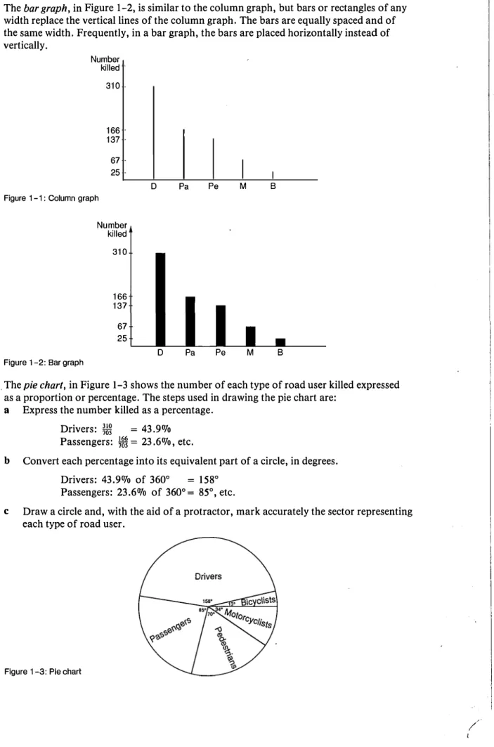
Height in cm Tally students (frequency)

150-

II

155- HH//1 8

160- HH fH++fH II 17

165-

HH fH+ H+r +Ht rlH Ill

170- _{rt+f f+H- I/ IJ} 14

175- H-HI 6

180-<185

+l+t

Total

Alternatively, we may use the

stem and

/ea/technique to classify the data. Each number

may be considered as consisting of two parts, the stem and the leaf. In the data in Example

3, in which the heights range from 150 to 185 cm, we may consider the first two digits of

each measurement as the stem and the units digit as the leaf. For example, for the first

observation (153), we may consider 15 as the stem and 3 as the leaf. However, this would

provide us with only four stems, namely, 15, 16, 17 and 18. Since we are dividing the data

into class intervals of 5 cm, it would be better to consider two stems fo! each of 15, 16,

17 and 18 and attach the units 0 to 4 with the first 15 and the units 5 to 9 with the second

15, and so on as follows:

Stem

15

15

16

16

17

17

18

Leaf

34

65999758

011 4302302433241 0

5779976589799568585979688659

1 3402401 41 2024

568975

34024

We may now place the leaves in ascending order, if desired. This then arranges the 80

observations in ascending order.

Stem Leaf

15

3 4

15

5 5 6 7 8 9 9 9

16

000011 1 2223333444

16 5555556666777778888899999999

17

000111 22234444

17

556789

18

02344

Total

2

8

17

28

1 4

6

5

80

The above frequency distribution shows the distribution of heights of a

sample

of 80

students. This sample may or may not be representative of the

population

of students of

this particular age group. We cannot generalise from the result of this sample, that two out

of

every

80 students of this age group would have a height in the range 150 - . The number

will vary from sample to sample.

12 STATISTICS

in this age group have heights from 150 cm up to, but less than, 155 cm or that the

probability of any student, randomly selected from this age group, having a height in this

range is 0.025. The probability of a student having a height of less than 160 cm is:

10

80 = 0.125.

In Table 1.2, the actual frequencies are expressed as percentage frequencies and

proportionate frequencies. For example, in the 150- class range, there are two students out

of 80, i.e. 2.50Jo or 0.025.

Table 1.2: Proportionate frequency distribution

Percentage

Proportionate

Height in cm

frequency

frequency

150- 2.5 0.025

155- 10 0.1

160- 21.25 0.2125

165- 35 0.35

170- 17.5 0.175

175- 7.5 0.075

180-<185 6.25 0.0625

Total

Frequency distributions, then, are sometimes of importance in themselves but they are

mainly important in providing information about the

population

from which the sample is

drawn.

Note:

The word 'population' does not necessarily refer to the entire population of a country or

even a State. It could refer to the population in a certain area or even in a particular school.

Furthermore, it does not necessarily refer to a population of people. We speak of, say, the

population of mass-produced electric light globes having varying lengths of life, or the

population of metal rods having varying diameters.

1.5 Histograms

A histogram is a diagram

representing the frequency

distribution of a continuous

variable.

The class limits are marked off

on a horizontal axis, and a

rectangle is constructed on each

class interval so that the

area

of

the rectangle is proportional to

the corresponding class

frequency. If the class intervals·

are equal, the heights of the

rectangles are proportional to

the frequencies.

Figure 1-6: Histogram

30

25

20

15

10

5

In the histogram in Figure 1-6, the height (and also the area) of each rectangle is

proportional to the frequency, because each class interval is the same.

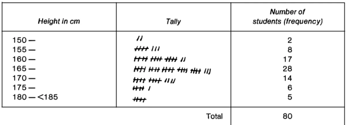
However, consider the following example. Table 1.3 gives the distribution of the diameters

of a large number of mass-produced wheels. Draw a histogram for these data.

Table 1.3: Percentage frequency distribution

Diameter Percentage

(cm) of wheels

4.86- 4

4.90- 6

4.92- 9

4.94- 20

4.96- 31

4.98- 20

5.02- 6

5.08-5.12 4

100

In Table 1.3 we notice that the class intervals are unequal. The most common class interval

is 0.02 cm. Taking this as the unit, and remembering that the area of each rectangle is

proportional to its corresponding class frequency, we notice that the 4. 86 - range has an

interval of 0.04, and so the height for this rectangle will be halved. Similarly for the 4.98

-and 5.08 - 5.12 ranges. The range 5.02- has a class interval of 0.06, -and therefore

we will have to take½ of the height of this rectangle (Figure 1-7).

32

28

24

Q)

20

'16

12

8

4

4.90 4.92 4.94 4.96 4.98 5.02 5.08 5.12 Diameter (centimetres)

1.6 Frequency polygons

In Figure 1-8, the polygon

ABCDEFGHI,

whose sides are straight lines joining the

midpoints of the tops of the rectangles of the histogram, is called

afrequency polygon.

Points

A

and

I

are the midpoints of the class ranges 145 - and 185 - respectively, which

have frequencies of zero. When the class intervals are equal, as they are in this case, the

frequency polygon encloses the same area as the histogram, but has a smoother form, and

so is sometimes considered to better depict the distribution in the population from which

the sample has been drawn.

30

25

(5'

20

10 5 147.5 ' B,,,' ' ' '

c/

Figure 1-8: Histogram and frequency polygon

Exercises 1 b

E " '' ' ' ' ' ' ' ' ' ' '

,/'

\

\

�/

\

,,/

:\

177.5 187.5

1 State which of the following are discrete variables (D) and which are continuous

variables (C)

a

The ages of the students in your class.

b

The number of goals scored by a soccer team.

c The lengths of the lives of electric light globes.

d

The number of accidents in a factory per month.

e

The number of errors per page in a book.

f The speed of a car in km I h.

g

The diameter of mass-produced metal rods.

2 The following numbers represent the heights, in cm, of 50 students.

152, 160, 168, 163, 170, 173, 151, 162, 166, 174, 165, 155, 166, 170, 169, 179,

165, 166, 176, 167, 167, 172, 169, 162, 156, 169, 169, 163, 166, 168, 160, 165,

171, 161, 167, 165, 157, 168, 175, 155, 171, 159, 158, 172, 163, 182, 162, 167,

168,164

a

Construct a frequency table using 5 cm as the class interval.

b Represent the data by means of:

3 The following are the marks scored by 40 candidates in an examination.

a Construct a frequency table with class intervals of 10 marks.

4

38 69 58 51 62 72 56 74 64 63

40 78 46 84 50 90 37 57 35 88

40 87 52 69 46 63 54 69 60 92

56 66 36 93 50 60 42 84 44 72

b

Depict the distribution by means of a histogram.

In estimating the value of a plantation of pine trees, the girths of the trees in a sample

area of 500 trees were measured, in cm, and the results were as shown.

Girth (cm) 30- 50- 70-

90-Number of trees 25 30 135 160

a

Convert the actual frequencies into relative frequencies.

b

Draw a histogram to represent the relative frequencies.

110-

130-100 40

150<170

10

c In a plantation of 800 trees, how many would be expected to have a girth of less than

70cm?

5

The frequency polygon on the right

shows the distribution of marks for

70 students in an examination.

�

20

18

16

6

Use it to construct a frequency

table.

Length of life

(hours) Frequency

300- 28

400- 60

500- 72

600- 92

700- 76

800- 50

900-<1000 22

Total

C

14

12

10

8

6

4

2

15 25 35 45 55 65 75 85 95

Marks

Percentage Relative frequency frequency

100 1

The frequency table above gives the lengths of the lives of 400 electric light bulbs tested

in a factory.

Answer the following questions:

7

c What percentage of bulbs failed in the first 500 hours?

d What proportion of bulbs had a life of at least 500 hours but less than 800 hours?

e If a similar batch of 600 bulbs were tested, how many would you expect to last for

at least 500 hours?

Frequently, for purposes of

comparison, histograms

(and bar graphs) are set out

horizontally, as shown on

the right in the age/ sex

pyramid of the population

of Victoria in 1986.

State any relevant

comparisons you can see

between the age

distributions of males and

females.

10

Age

75

70 74

65 69

60 64

55 59

50 54

45 49

40 44

35 39

30 34

25 29

20 24

15 19

10 14

5 9

0 4

Females

5

10

8 Draw histograms for the population of Victoria in 1959 and 1982, as tabulated below,

and make some relevant comments. Populations are given to the nearest thousand. (Set

out your histograms horizontally as in Question 7 .)

Age group

0-9

10-19 20-29

30-39 40-49

50-69 70-89

Population 1 959

574

453

368

426

359

490

145

Population 1 982

612

706

674

598

427

716

260

9 Use a histogram and a frequency polygon to represent the following data relating to

the civilian labour force, by age, in Victoria in 1987. The number of people is expressed

to the nearest thousand in this table:

Age group

15-17 18-19 20-24 25-34 35-44 45-54

55-59

60-64 �65

Persons

1. 7 Measures of central tendency

So far we have been concerned only with the graphical representation of statistical data.

Frequently we use the

average

of a set of data to represent the data. For example, we talk

of the average height of a group of students, the average mark of the class in an

examination, or the average wage of workers.

This magical word 'average' is not the smallest or the largest value of a variable but tends

to lie centrally in the set of observations and so is called a measure of

central tendency.

The

three most commonly used measures of central tendency are:

a the

mode

b

the

median

c

the

arithmetic mean

or, simply, the

mean

The mode

The mode of a distribution is the most frequent or most popular value of the variable.

For the observations 6, 7, 7, 5, 8, 6, 7, 9, 7, 4, 7, the mode is 7 because this number occurs

more frequently than any other number.

In Table 1.1, the mode of the distribution lies approximately in the middle of the class

interval 165 - , i.e. at the value 167 .5 cm. The 165 - class is called the

modal class.

In Table 1.2, the mode is 4.97 cm approximately, and the 4.96 - class is the

modal class.

Some distributions may have more than one mode. If their histograms have two well defined

humps, the distribution is said to be

bimodal.

If the histogram has one hump only, as in

Figures 1-6 and 1-7, the distribution is

unimodal.

The median

Discrete data

The median of a set of observations is the middle number when the numbers are arranged

in order of magnitude, or is halfway between the two middle numbers if there is an even

number of observations.

Example 4

Find the median of

a 6, 7, 7,5,8,6, 7,9, 7,4, 7

b 8,4, 10,2,6,9, 8,5

a Arranging the numbers in order, we get:

4, 5, 6, 6, 7, 7, 7, 7, 7, 8, 9

I

The median is 7

b

Arranging the numbers in order, we get:

2, 4, 5,�8, 9, 10

The two middle numbers are 6 and 8.

Continuous data

The frequency distribution in Table 1.1 can be converted to a

cumulative frequency

distribution

by adding each frequency to the total of its predecessors.

Table 1.4: Cumulative frequency distribution

Height in

Cumulative

cm

frequency

< 150 0

< 155 2

< 160 10

< 165 27

< 1 70 55

<175 69

< 180 75

< 185 80

Table 1.4 shows, for example, that: 55 out of the 80 students have heights less than 170 cm;

11 have heights equal to or greater than 175 cm; and so on.

80

70

60

� 50

Q)

>

:;::, _ca ::i

40

---0 3---0

20

10

167.5

0--'-=---'--_i_--L-...L__L __ L_ _ _J_ __ ...1_ _ __..

150 155 160 165 170 175 180 185 Height (cm)

Figure 1-9: Cumulative frequency curve

The graph of a cumulative frequency distribution is called a

cumulative frequency curve

or

ogive.

The 0.5 quantile, for example, is the value of the variable below which½ of the distribution

falls.

The 0.5 quantile is called the

median.

The median can be found from the cumulative frequency curve. Its value is approximately

167.5 cm. So one half of the 80 students has a height of l_ess than 167 .5 cm.

Quantiles,

when expressed as a percentage, are called

percentiles.

The 0.8 quantile is the

80th percentile and, from the cumulative curve, its value is 173 cm. So 80 per cent of the

students have heights less than 173 cm. It is advisable to draw the cumulative curve on graph

paper so that the quantiles may be read with reasonable accuracy. The 25th percentile or

0.25 quantile is called the

lower quartile,

below which¼ of the observations lie. The 75th

percentile or 0. 75 quantile is called the

upper quartile,

below which¾ of the observations

lie.

Box plots

A useful method of illustrating the range, the median and the upper and lower quartiles

is by means of a

box plot,

sometimes called a

box-and-whisker

diagram.

In Example 4a, the 11 observations range in value from 4 to 9. The median, m, is 7, below

which there are five observations, namely:

4 5 6 6 7

The middle of this set is 6. This is the lower quartile,

L.

The upper quartile,

U,

is the middle

of the upper five observations:

7 7 7 8 9

The upper quartile is, therefore, 7. The interquartile range is from 6 to 7.

In Example 4b the eight observations range in value from 2 to 10. The median is 7, below

which there are four observations: 2, 4, 5 and 6. The middle of this set is 4.5. This is the

lower quartile,

L.

The upper quartile,

U,

is the middle of the upper four observations: 8,

8, 9 and 10. The upper quartile is 8.5.

The interquartile range is from 4.5 to 8.5. In a box plot, the interquartile range is boxed

as shown in Figure 1-10. The lines drawn from the box to the extreme values are the

whiskers.

a

b

L

2 3 4 5 6

Figure 1-1 O

L U

M M

7

u

8 9 10

The two distributions can be compared and contrasted by.drawing their box plots together

and noting the comparative lengths of the boxes and the whiskers. What conclusions can

you draw from box plots a and b in Figure 1-10?

In Example 3, the heights, to the nearest centimetre, of 80 VCE students were given. Their

heights ranged from 153 cm to 184 cm, �s shown in the stem and leaf method of arranging

the data in ascending order. The lower and upper quartiles are 162 and 171 respectively,

and the median is 167. Check these from the cumulative frequency curve (Figure 1-9) or

from the stem and leaf presentation of the data. The box plot is shown in Figure 1-11.

L M

150

155

160

165

Figure 1-11

u

170

Height (cm)

175

180

185

190

The whiskers appear to be long compared with the length of the box. What conclusions can

be drawn?

Arithmetic mean

The mode and quantiles are

typical values

of a distribution. Some of these typical values,

e.g. the mode and the median, are measures of

central tendency.

Another measure of central

tendency is the

arithmetic mean.

The arithmetic mean, or simply the mean, is the average of a set of observations.

Ungrouped data

The mean of a set of n observations x

x2, ... x

is denoted by x (read 'x bar') and is

defined by:

X = X1

+

X2 + X3 + , , ,

n

+

X11

Ex

n

Ex (called sigma x) is the sum of the values of the statistical variable.

Example 5

The mean of the numbers 3, 4, 8, 9, 11 is:

x=3+4+8+9+11

5

= 35 = 7

5

Grouped data

If the numbers x,, x2, X3, ... , Xk occur J,,h,h,

. . . ,

/k times respectively, the arithmetic

mean is:

-

xif, + Xz/2 + Xy3 + , , , + Xk/k

x=�--�- -

J,

+

h

+

h

-"---=--+ ... -"---=--+

/k

= Exf

Ef

Exf

Example 6

Calculate the mean height of the 80 students in Table 1.1.

Since two students have heights in the range from 150 cm up to, but less than,

155 cm, we take the middle of this class range, 152.5, as representing the average

height of the two students, and so on for the others, as shown in Table 1. 5 below.

Table 1.5

Height in Number of cm,x students,/

152.5 2

157.5 8

162.5 17

167.5 28

172.5 14

177.5 6

182.5 5

'f:.f

xf

Exf = 13 410

- -M

X

f,f

13410

80

=

167.6 (cm)

It is obvious from the symmetry of this distribution that the mean is around 167.5,

in which case, the arithmetical calculation can be simplified by making 167 .5 the

origin and creating a new variable,

V.

The relation between

x

and Vis given by

the equation

x

=

a

+

kV,

where

a

is the origin, 167 .5, and

k

the class interval, 5.

Table 1.6

V

f

-3 2 -2 8 -1 17 0 28 1 14 2 6 3 5 80 VJ - 6 -15 -17 0 14 12 15 2

x =a+ kV

2

=

167.5 + 5 X 80

= 167.5 + 0.1

=

167.6(cm)

Example 7

The marks out of 10 gained by the two top students, Gwen and Nick, for a series of ten

maths tests throughout the year are as follows:

Test

1

3

4

6

7

8

10

Gwen

10

10

7

10

10

10

Nick

10

8

8

8

7

10

Who should receive the maths prize for the best maths student of the class?

Arranging their scores in order we get:

Gwen: 2, 7, 9, 9, 9, 10, 10, 10, 10, 10.

Nick: 7, 8, 8, 8, 9, 9, 9, 9, 10, 10.

Total 86

Total 87

Table 1. 7 shows their mean, mode and median scores.

Table1.7

Gwen

Nick

Mean

8.6

8.7

Mode

10

Median

Total

86

87

Nick argues that he should receive the prize because his total score, and therefore his mean

score, for the ten tests is higher than Gwen's.

Gwen argues that she should receive the prize because both her mode score and her median

score are higher. Furthermore her score is equal to or greater than Nick's in seven out of

the ten tests - equal in two tests and greater in five tests. Why should she lose the prize

because of a mark of 2 in the ninth test?

The

mean

is the most commonly used measure of central tendency because it takes all of

the observations into account. However, it can be seriously influenced by any extreme values

such as Gwen's score of 2 in the ninth test. The mode and median are not altered by any

extreme values and in some situations are better measures of central tendency. A

manufacturer, for example, would consider the

mode

to be the most important. Why?

In a survey of incomes, for example, the

median

income would give a clearer indication of

the situation than the

mean

because of the few people who would have very high incomes

compared with the majority. In situations like this, it is a common practice to eliminate the

upper and lower quarter of the distribution and calculate the mean for the inter-quartile

range.

1.8 Measurement of dispersion

The mean, median and mode give one aspect of frequency distributions, namely

central

tendency,

and are often called

measures of location

because they locate some central value

of the distribution. However, they give no information about how the observations in a

sample are spread about their central values. The two sets of observations:

both have the same mean, 9, but the second set has more spread.

It

is important, then, to

have some method (or methods) of measuring spread or dispersion.

1 The range

The range is the difference between the greatest and least values in a distribution.

It

has a

limited usefulness, since it takes into account only the two extreme observations and ignores

a possible concentration of values around a typical value.

2 The inter-quartile range

The inter-quartile range is the difference between the upper and lower quartiles. It is used

to indicate the spread of the middle half of the observations and is useful in many situations

which wish to ignore extreme values.

3 Variance and standard deviation

The variance and standard deviation are the measures of dispersion most frequently used.

(i) Ungrouped data

The variance of a set of n observations x1, x2, X3 .•. X

is denoted by s2 and is defined by:

The standard deviation is the positive square root of the variance and is defined by:

s = �E(x - x)

n - I

where E(x - x)

represents the sum of the squares of the deviations of the n observations

from the mean, x.

(ii)

Grouped data

If the numbers

xi,

X2, X3, ••• , Xk occur with frequenciesfi,f2,h, ... ,fk, the variance

is defined by:

s

= E(x -

x>

2

f, where n = Ef

n

- I

The standard deviation is defined by:

Example 8

Calculate the standard deviation of the observations 1, 2, 6, 7, 9.

The following steps are followed:

a calculate the mean of the set of observations.

b calculate the deviation of each observation from the mean.

c square these deviations and find the sum of the squares.

d calculate the square root of the sum of these squares divided by

n

- 1.

X

x-x

1

-4

2

-3

6

1

7

2

9

4

Total

25

M

ean,x = 5 =

-

25 5

The standard deviation, s,

is given by:

s

= .

/E(x

- x)

'Y

n

- 1

=ii

=

-./TIT

= 3.391

The variance, s

= 11.5

Example 9

(x

-

x)

16

9

1

4

16

46

Calculate the standard deviation of the following frequency distribution.

· '

0

1

X

f

12

29

X

f

0

12

1

29

2

26

3

18

4

10

5

5

Total

100

x =

Exf

n

= 200 = 2

100

2

4

5

26

18 10

5

xf

x-x

(x

-

x)'f

0

-2

48

29

-1

29

52

0

0

54

1

18

40

2

40

25

45

Note:

The standard deviation, s is given by:

s

= _ /I;(x

- x)

f

'V

n

-, 1

=

�180

99

= .JT]Ts

The variance, s

=

1.818

The divisor in the formula for the standard deviation is

n

- 1 and not

n.

The reason for

this could, perhaps, be given at this stage by stating that the first observation clearly tells

us nothing about the variability in the sample, so that only

n

- 1 of the

n

observations

are available for estimation of this variability. Furthermore, only

n

-

1 of the

n

deviations

from the mean are independent.

Many distributions are approximately of the

normal

type with a fairly well defined

symmetrical tendency with:

(i)

practically all of the observations in the range x ± 3s.

(ii)

about 95 per cent of the observations in the range x

±

2s.

(iii)

about� of the observations in the range

x

±

s.

Exercises 1c

1 A survey of the number of children per family of 20 families in a particular area

produced the following results:

0, 4, 1, 0, 2, 5, 3, 3, 2, 1, 4, 6, 2, 3, 1, 3, 4, 3, 1, 3

a Calculate the mean, mode and median.

b Draw a box plot of the data.

2 A proofreader recorded the number of errors per page in a 40-page document as

follows:

Number of errors

₀

1

Number of pages

"12

10

a Calculate the mean, mode and median.

b Draw a box plot of the data.

2

3

4

7

5

4

5

2

3 A survey of the rent paid per week by 100 tenants in a Melbourne suburb recorded the

following data:

Weekly rent($)

60-

65-

70-

75-

80-Frequency

6

8

9

20

30

a Estimate the mean rental.

b Draw a cumulative frequency curve, and from it estimate:

(i)

the median rental

85-15

(ii)

the proportion of tenants paying more than $76 per week.

c Draw a box plot of the data.

90-

95-100

4 The following table shows the age distribution of 60 female workers in a clothing

factory.

Age

20-

25-

30-

35-

40-

45-

\

50<55

Frequency

4

8

13

11

a Estimate the mean age.

b

Draw a cumulative frequency curve and from it estimate:

(i)

the median age

(ii)

the 0.8 quantile

(iii)

the number of workers aged less than 32.

10

I

5

5 Over the past year, there were 120 accidents in a manufacturing company with

subsequent loss of production time. The number of worker-hours lost per accident is

shown in the following table:

Number of hours

lost per accident

0-

5-

10-

15-

20-

25-

30<35

Number of

accidents

17

25

38

20

9

7

4

a Estimate the mean number of hours lost per accident.

b For what percentage of the accidents was the number of hours lost per accident

between 5 and 25 hours?

6 Transistors are sold to customers in cartons containing 10 transistors. The following

table shows the number of defective transistors per carton in a sample of 100 cartons.

Number defective per carton

Number of cartons

Calculate:

, .

0

57

a the mean number defective per carton

b

the mode

c

the median

1

2

3

4

30

10

2

1

7 The table below shows the percentage distribution of deaths from scarlet fever among

the various age groups:

Age in years

0-

1-

2-

3-

4-

5-Percentage of deaths

6

14

17

20

12

8

Age in years

6-

7-

8-

10-

15-20

Percentage of deaths

7

7

2

2

4

1

a Construct a cumulative percentage frequency distribution and draw the cumulative

curve.

8

The following table gives the distribution of the diameters of a large number of mass­

produced wheels.

Diameter (cm)

4.86-

4.90-

4.92-

4.94-Percentage of wheels

2

6

9

20

Diameter (cm)

4.96-

4.98-

5.02-

5.08-5.12

Percentage of wheels

31

20

8

4

Construct a cumulative percentage frequency distribution and draw the cumulative

curve. Use the curve to estimate:

a the median diameter.

b the 0.9 quantile.

c the proportion of wheels expected to have a diameter of not less than 4.95 cm.

9 The following table shows the frequency distribution of the marks of 600 candidates

in an examination.

Marks

1-10

11-20

21-30

31-40

41-50

Number of

candidates

5

30

60

105

130

Marks

51-60

61-70

71-80

81-90

91-100

Number of

candidates

100

75

50

30

15

Construct a cumulative percentage frequency curve and answer the following questions:

a

What is the interquartile range?

b

If the pass mark is 45, what percentage of the candidates passed?

c

If honour passes were given to the top 20 per cent of candidates, what would be the

lowest mark required to obtain an honour?

10

For the following set of observations, calculate:

a

the mean

b the standard deviation:

9,6,8,6, 7, 7,6,4, 7, 7,8,9.

11

Calculate the

standard deviation

of these observations:

45,40,42,40, 38

12

In testing two modifications of an existing eyepiece design in a microscope, an observer

took 10 readings of a fixed length with each eyepiece. The results were as follows:

Design A: 295,278,289,304,293,307,293,290,296,300.

Design B: 276, 266, 273, 286, 276, 268, 238, 252, 290, 242.

It is required to know whether:

a

readings with one design are more consistent than with the other.

b

one eyepiece produces readings that are generally lower than those obtained by using

the other.

13

The egg production from two pens of fowls, taken from a total hatching of 1000 fowls,

was recorded over a period of 90 days. The first pen contained 50 birds and produced

an average of 36.4 eggs per day. The birds in the second pen, which numbered 80,

produced an average of 69.3 eggs each in the period. Estimate the total production from

the 1000 birds over the period.

Under what conditions is this estimate justified?

14

Each of 26 students in a class measured

the lengths of th