Volume 2006, Article ID 74838, Pages1–16 DOI 10.1155/ASP/2006/74838
Knowledge-Aided STAP Processing for Ground Moving
Target Indication Radar Using Multilook Data
Douglas Page and Gregory Owirka
BAE Systems Advanced Information Technologies, 6 New England Executive Park, Burlington, MA 01803, USA
Received 7 November 2004; Revised 16 February 2005; Accepted 8 March 2005
Knowledge-aided space-time adaptive processing (KASTAP) using multiple coherent processing interval (CPI) radar data is de-scribed. The approach is based on forming earth-based clutter reflectivity maps to provide improved knowledge of clutter statistics in nonhomogeneous terrain environments. The maps are utilized to calculate predicted clutter covariance matrices as a function of range. Using a data set provided under the DARPA knowledge-aided sensor signal processing and expert reasoning (KASSPER) Program, predicted distributed clutter statistics are compared to measured statistics to verify the accuracy of the approach. Robust STAP weight vectors are calculated using a technique that combines covariance tapering, adaptive estimation of gain and phase corrections, knowledge-aided prewhitening, and eigenvalue rescaling. Techniques to suppress large discrete returns, expected in ur-ban areas, are also described. Several performance metrics are presented, including signal-to-interference-plus-noise ratio (SINR) loss, target detections and false alarms, receiver operating characteristic (ROC) curves, and tracking performance. The results show more than an order of magnitude reduction in false alarm density when compared to standard STAP processing.
Copyright © 2006 D. Page and G. Owirka. This is an open access article distributed under the Creative Commons Attribution License, which permits unrestricted use, distribution, and reproduction in any medium, provided the original work is properly cited.
1. INTRODUCTION
The lack of training data in nonhomogeneous clutter envi-ronments can cause severe degradation in the performance of space-timeadaptive processing (STAP) algorithms (see [1,2] and references therein). Surveillance radars typically perform STAP processing [3] on a limited number of pulses of data, which are referred to as a coherent processing interval (CPI). Each CPI is divided into a number of time samples which correspond to the radar range gates. In each range gate, the return signal in each antenna channel and on each pulse in the CPI is digitized into in-phase and quadrature compo-nents. The radar returns can thus be represented as complex numbers, whose real parts are the corresponding in-phase components, and whose imaginary parts are the quadra-ture components. Thus, in each range gate the returns from each channel and pulse can be represented as an NM by 1 complex column vector, where N is the number of an-tenna channels andM the number of pulses per CPI. Co-variance estimation for STAP is usually performed by aver-aging the outer products of these return vectors with them-selves over a number of training range gates from a single CPI. As was shown by Reed et al. [4], this is a maximum like-lihood estimate of the clutter covariance matrix, assuming
zero-mean complex Gaussian and homogeneous (i.e., range-independent) statistics.
Due to varying terrain conditions, the covariance esti-mation just described may result in poor estimates, due to an inadequate amount of training data matching the range gate under test. Two possible consequences of this are under-nulling or overunder-nulling of clutter. Underunder-nulling may occur if the test range gate contains strong clutter due to, say, steeply sloped terrain, while the training window surrounding the test cell contains less severe clutter. This may lead to an exces-sive number of false alarms or, if the threshold is increased to reduce false alarms, loss of target detections. Overnulling of clutter may occur when the training window contains steeply sloped terrain or windblown clutter that is not present in the target range cell. Overnulling leads to the loss of target detec-tions.
of clutter scattered from a given point on the ground will also be changing. Moreover, the area of intersection between the radar resolution cells and the earth’s surface will also be changing with platform geometry. Thus, simply averaging outer products of complex returns from additional CPI data cubes to augment standard covariance estimation is not ef-fective (and may in fact cause STAP performance to degrade rather than improve).
Additionally, in actual ground moving target indication (GMTI) surveillance systems there are a number of real-world effects that can degrade the performance of knowl-edge-aided STAP techniques. Unknown antenna pattern mismatch and internal clutter motion can cause model er-rors and undernulled residual clutter. High ground target densities produce target contamination of the STAP training data, thus producing filter nulls at the locations of the de-sired targets. Returns from large discretes, such as buildings in urban areas, are spatially localized and can be much larger than the returns from distributed clutter. These returns can cause numerous false alarms that are spread over a wide area due to sidelobe effects. Effective suppression of such discrete returns may require specialized techniques in addition to those used for distributed nohomogeneous clutter.
In order to exploit multilook radar data, an effective knowledge-aided STAP approach must be able to extract in-formation from each CPI on clutter statistics, correct for CPI-to-CPI differences in the statistics, and calculate STAP weight vectors that are robust under real-world GMTI condi-tions. Our approach to accomplish these objectives combines a number of different techniques, which are listed below:
(1) formation of earth-referenced clutter reflectivity maps using multiple CPIs,
(2) covariance tapering to model internal clutter motion [5],
(3) extended-factored (or “adjacent bin”) post-Doppler processing [6],
(4) adaptive estimation and correction for channel and Doppler-dependent gain and phase errors,
(5) knowledge-aided prewhitening using the colored load-ing technique of [7,8],
(6) eigenvalue rescaling of the knowledge-aided covari-ance matrix,
(7) masking of STAP training data using a two-pass proce-dure to reduce the effects of targets on the covariance estimates,
(8) specialized processing to detect and remove returns from large discretes such as buildings.
We have listed where appropriate references by other au-thors that are employed in each technique. Covariance ta-pering is described in [5] and is applied to the covariance matrices derived from the clutter reflectivity map. This mod-els the effects of internal clutter motion (ICM), which is an important real-world phenomenon. We used post-Doppler STAP degrees of freedom known as extended-factored or adjacent-bin post-Doppler STAP [6]. The knowledge-aided prewhitening algorithm developed by Bergin et al. [7,8] is also an important part of the approach. However, we have
also found the nonreferenced algorithm components listed above that we developed (i.e., techniques (1), (4), (6), (7), (8)) to improve STAP performance significantly. In addition, we consider a performance metric not normally shown in the literature. In addition to the usual signal-to-interference-plus-noise ratio (SINR) loss metric, we also study the resid-ual clutter-to-noise ratio (CNR) after STAP processing. The latter is especially important, as it determines the number of false alarms that will be observed after constant false alarm rate (CFAR) processing is performed. To further quantify the benefits of our approach we also show receiver operating characteristic (ROC) curves of detection probability versus false alarm density.
An outline of the paper is as follows. We describe in Section 2techniques (1)–(6) in detail. InSection 3, we con-sider target contamination effects (technique (7)) and show the results of processing the KASSPER Data Set 2 [9]. The results obtained indicate that significant improvements in STAP performance may indeed be achieved by incorporating multiple CPI data cubes into knowledge-aided STAP process-ing usprocess-ing the approach we describe. InSection 4, we show the degrading effects of strong clutter discretes on GMTI KASTAP performance. We describe additional KASTAP tech-niques for suppressing these discretes and show results that indicate these techniques are effective in eliminating the degradation caused by large discretes. Finally,Section 5 sum-marizes our results.
2. ALGORITHM DESCRIPTION FOR DISTRIBUTED
CLUTTER MITIGATION
2.1. Formation of clutter reflectivity maps
The first aspect of our KASTAP approach using multilook radar data is to form earth-referenced clutter reflectivity maps. The goal of this step is to extract estimates of clut-ter return strength as a function of spatial location on each CPI and to incorporate these estimates into a clutter map defined in a single common coordinate system. This com-pensates for the differences in the radar coordinate systems on each CPI and allows information on clutter statistics de-rived from multiple CPI looks to be utilized in determining the STAP filter weights on subsequent CPIs. By incorporat-ing estimates from multiple CPIs over an extended time pe-riod, the effects of random estimation errors and target con-tamination effects on the clutter return estimates are reduced through the averaging process.
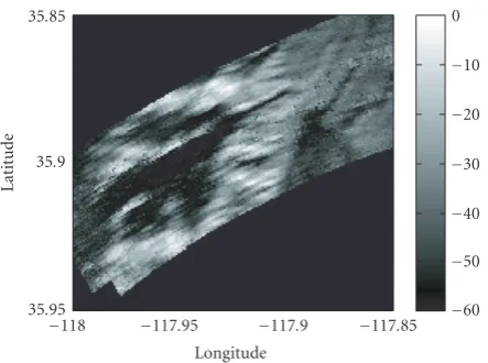
As illustrated inFigure 1, there are four basic steps in-volved in forming a clutter reflectivity map from multiple CPI data cubes. These steps are described individually below.
2.1.1. Definition of clutter scatterers
Multiple CPI datacubes
Define range/Doppler locations of clutter scatterers
Georegister & estimate scattering
strengths
Normalize & form average earth-based reflectivity map DTED &
platform geometry
Longitude
Latitude
35.95 35.9 35.85
−118 −117.95 −117.9 −117.85 0
−10
−20
−30
−40
−50
−60
Figure1: Illustration of procedure for forming an earth-based clutter reflectivity map.
Table1: KASSPER Data Set 2 parameters [9].
Quantity Value
Radar frequency 10 GHz Radar bandwidth 10 MHz
Peak power 10 kW
System losses 7 dB
Antenna size 1.43 m (horizontal) by.285 m (vertical)
Transmit antenna pattern Spoiled to 10-degree beamwidth Receive antenna
configuration
12 nonoverlapping subarrays, spaced by 4 wavelengths per subarray
Number of pulses per CPI 38
Number of CPIs per dwell 3 with PRFs of 2081, 1800, and 1518 Hz
Time separation of dwells 10 s Number of dwells
in scenario
30
Platform motion 150 m/s, heading west
Crab angle 3◦
Standoffrange to targets Approximately 45 km Target clusters 3 clusters, 60 vehicles each Background traffic 1000 vehicles
Target motion Move along roads, speed 2–25 m/s depending on road type, decelerate when approaching intersections Earth model Spherical, radius 6 378 388 m,
mod-ulated by DTED
large buildings in urban areas, will be considered separately inSection 4. To motivate the distributed clutter environment model, we first discuss the characteristics of the KASSPER Data Set 2 that was processed. The parameters for this data set are given inTable 1.
The antenna elements of the KASSPER Data Set are formed using 12 nonoverlapped subarrays spaced by 4 wave-lengths per subarray. The subarrays are presteered to a partic-ular direction on each CPI. The azimuth and elevation angle of this presteering direction are supplied along with the data
cube for each CPI. Each CPI contains 38 pulses, and a dwell consisting of three consecutive CPIs at different pulse rep-etition frequencies (PRFs) occurs every 10 seconds. During this time interval, the platform moves 1.5 km. This is signif-icant relative to the 40 km standoffrange to the targets, as small CPI-to-CPI changes in aspect angle can produce large changes in the space-time response of clutter scatterers.
With the parameters shown inTable 1, a Doppler reso-lution cell located broadside to the platform spans approxi-mately 0.3 degrees in azimuth. This is a factor of 4 finer than the antenna beamwidth of 1.2 degrees. Thus, the Doppler fil-ter spacing is about 1/4 of the antenna beamwidth (as one moves offbroadside, the Doppler filter width and antenna beamwidth are both inversely proportional to the cosine of the azimuth steering angle). Consequently, modeling the clutter environment as a set of point scatterers spaced apart by no more than one Doppler filter should result in oversam-pling of the radar azimuth resolution. The bandwidth of the system shown inTable 1leads to a range resolution of 15 m, which is much smaller than the size of the antenna beams or Doppler filters on the ground. Thus, one scatterer per range cell should suffice to give accurate clutter statistics.
The Doppler extent of the scatterers assumed in each range gate is limited by the fact that the spatial response across the antenna subarrays has grating lobes due to the 4 wavelength spacing. If the extent is selected to be too large, the space-time response of two different clutter scatterers can become nearly the same due to the simultaneous presence of a temporal (Doppler) and spatial ambiguity. This would pre-vent accurate estimation of the relative scattering strengths of the two scatterers. In order to avoid this problem while sim-ulating the effects of sidelobe clutter, scatterers were selected to span the main Doppler ambiguity plus 30% of each of the Doppler ambiguities on either side of the main ambiguity.
2.1.2. Georegistration of clutter scatterers
estimates from multiple CPIs, we define a common earth-based coordinate system. The process by which the location of the model clutter scatterers from a given CPI on the earth is determined is referred to as georegistration. The ground location of a clutter scatterer is defined by the intersection of three surfaces:
(a) a range sphere centered on the platform location, hav-ing a radius equal to the slant rangeRsof the scatterer, (b) a cone about the platform velocity vector, correspond-ing to the Doppler frequency of the scatterer. Neglect-ing internal clutter motion, the cosine of the cone an-gle relative to the platform velocity vector is given by
cosθc=λ f
dop
2Vp , (1)
where λ is the radar wavelength, fdop the scatterer
Doppler frequency, andVpthe radar platform speed, (c) the earth’s surface. This is defined by digital terrain
el-evation data (DTED).
The height of the earth’s surface at a scatterer location de-pends on its latitude and longitude, and these are unknown. An iterative approach using an initial estimate of the terrain heighthabove the reference spherical earth model of radius
Rewas employed. Let the unknown position of the scatterer in earth-centered coordinates be denoted byrsc. The
plat-form position vector is known and is denoted by rp. The scatterer position is then determined by solving the follow-ing three equations:
rsc−rp2
=Rs2 (range sphere),
rsc−rp
•vp=Rs·Vp·cosθc (Doppler cone),
rsc2
=Re+h
2
(earth sphere).
(2)
The above equations constitute a set of three equations and three unknowns, which are the three components of the scat-terer position vectorrsc. To refine the value ofh, the
earth-centered position vectorrscis converted to latitude and
longi-tude using spherical earth geometry. The new terrain height is then obtained by accessing the DTED database at this lo-cation. Several iterations of this procedure were employed to reduce the geolocation error to a small fraction of a res-olution cell. For the study described in this paper, a level 1 database indexed by latitude and longitude having a post-ing of 90 m was employed (note from Table 1 that in the KASSPER Data Set these height variations occur on a refer-ence spherical rather than ellipsoidal earth).
2.1.3. Estimation of scatterer strengths
Once the scatterer locations on the ground are determined, their contributions to the received radar amplitudes must be estimated. This first requires defining the space-time steering vectors to each scatterer. Assuming identical antenna chan-nels, the elements of a steering vector are a known function of the look direction to the scatterer and its Doppler frequency. The magnitude of the steering vector elements is also scaled
by the overall (channel-independent) subarray azimuth an-tenna gain on the scatterer. This is done in order to correct for known CPI-to-CPI changes in this antenna pattern, and it is important for clutter scatterers that are near the edge of the mainlobe region of the subarray pattern. As the platform geometry changes, such scatterers can move into the main-lobe and produce a significantly larger return, or move into the sidelobe region and produce a weaker return. (We only assume that the overall pattern is known and is the same for all the antenna channels; to account for channel mis-match we have an adaptive procedure that will be described inSection 2.3.3.)
Let the steering vector to the scattereriin a given range gate of a given data cube be denoted bysi. Also letxbe the measured data vector in the range gate. We desire an approx-imation toxin the form
x=
i
αi·si. (3)
The complex return strengthsαiare selected in order to min-imize the squared error
ε=x− i
αi·si
2. (4)
The solution of this problem can be shown to be
αi=
j
S−1i j·sjHx, [S]i j≡siHsj. (5)
In general, the matrixSwill not be diagonal, due to the fact that the steering vectors will not be orthogonal. This is true even if the scatterer spacing is selected to be one Doppler filter, due to the fact that multiple Doppler ambi-guities are modeled. The complex numbersαirepresent the return strengths and phases of the scatterers in a given range gate of a given data cube. Each of the scatterers represents clutter in one range-Doppler cell, which in turn corresponds to a particular area on the ground. The procedure described here is repeated for all the processed range gates in each of the CPI data cubes used to form a clutter reflectivity map.
2.1.4. Normalization of clutter reflectivity
Since the complex clutter estimates described inSection 2.1.3 are derived from measured data, they implicitly include all the effects of parameters appearing in the radar range equa-tion (i.e., transmit antenna patterns, clutter radar cross sec-tion, etc.). The cell areas of range-Doppler resolution cells on the ground are different on each CPI, due to the diff er-ent pulse repetition frequencies (PRFs), as well as the chang-ing geometry as the platform moves. Because the areas are changing from CPI to CPI, it is important to build the clutter reflectivity map using reflectivity, which normalizes the clut-ter return power by the cell area. DefineΔrrng(i)as the vector
The area of the corresponding ground cell is then given by
Ai=Δrrng(i)×Δrdop(i). (6)
The clutter reflectivity of the scatterer is then defined as the estimated clutter power|αi|2 divided by the area on the
groundAirepresented by that scatterer.
2.1.5. Formation of clutter reflectivity maps
The reflectivity maps are built by first determining, for each cell of the map, the range and Doppler indices of the clut-ter scatclut-terer that encompasses the cenclut-ter of the cell on each CPI. This is accomplished using a straightforward conver-sion from earth-centered coordinates to radar-centered co-ordinates. The clutter reflectivity of the cell is then calcu-lated by averaging the estimated reflectivities of the corre-sponding scatterers over many CPIs. To improve the fidelity of the reflectivity map, reflectivity estimates from the cur-rent CPI are incorporated adaptively. It is important to in-clude current-CPI data, since as the platform moves new ar-eas on the ground may contribute significantly to the clut-ter inclut-terference. Additionally, large changes in clutclut-ter reflec-tivity will occur when a ground patch first becomes visible to the radar (producing an increase) or shadowed from the radar by terrain (producing a large decrease in reflectivity). To improve the clutter reflectivity estimates under these con-ditions, a metric was formulated to detect such changes.
Assume that we have individual clutter reflectivity esti-mates in a given cell of a ground-based reflectivity map onL
past CPIs. These estimates are denoted asrl,l= 1, 2,. . .,L. We also have a reflectivity estimaterL+1 on the current CPI.
We assume that eachrl is a random variable with an expo-nential probability distribution. This is justified by the fact that these estimates are derived as thesquared magnitude of a linear combination of complex Gaussian random variables. To detect reflectivity changes, we define two hypotheses:
H0:rL+1 has the same mean asr1,2,...,L,
H1:rL+1 has a different mean thanr1,2,...,L.
The generalized likelihood ratio test (GLRT) for deciding be-tween the two hypotheses (see [10] for a good description of this technique) can be easily shown to have the form
(L+ 1)·ln
L+1
l=1rl
L+ 1 −L·ln
L l=1rl
L −lnrL+1> TG. (7)
Here,TGis the GLRT threshold setting. Normally, the reflec-tivity map cell value is set equal to the averageLl=+11rl/(L+ 1) of the estimated reflectivities over all the CPIs processed. When the GLRT threshold is exceeded, however, the map reflectivity is set equal to the current-CPI estimaterL+1. In
this manner, the reflectivity map responds more rapidly as a function of time (CPI) to rapid changes in clutter return strength. A similar approach has been used in [11] to per-form SAR change detection.
35.95 35.9 35.85
Latitude
−118 −117.95 −117.9 −117.85 0
−10
−20
−30
−40
−50
−60 Longitude
Figure2: Clutter reflectivity map formed from multiple CPIs of the KASSPER Data Set 2.
Figure 2shows a clutter reflectivity map that was calcu-lated using CPI #s 17–22 of the KASSPER Data Set 2, with adaptive GLRT processing on CPI #22. The resolution of the map was selected as 25 m, which is slightly larger than the 15 m range resolution. The boundaries of the map corspond to the range limits processed on each CPI. The re-flectivity map is seen to predict regions of very strong clut-ter, which are produced by steeply sloped terrain. In addition there are areas where the reflectivity is much weaker, which includes regions that are shadowed from the radar (i.e., not visible). The knowledge gained from the reflectivity map al-lows these areas to be identified. The STAP processor can in-corporate this knowledge into the adaptive weight vector and reduce the magnitude of over-/undernulling that occurs with standard range-averaged covariance estimation.
2.2. Prediction of current-CPI statistics
70 60 50 40 30 20 10
Doppler
inde
x
50 100 150
Range gate
20 30 40 50 60 70 80
(a)
70 60 50 40 30 20 10
Doppler
inde
x
50 100 150
Range gate
20 30 40 50 60 70 80
(b)
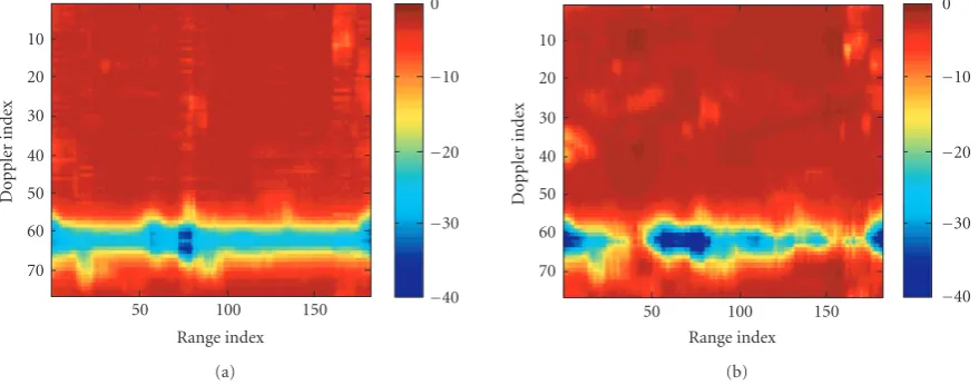
Figure3: Comparison of (a) measured range-Doppler spectrum for CPI #22 with (b) prediction of clutter reflectivity map.
map. To obtain the estimated powerpiof scattereri, the re-flectivity is multiplied by its cell areaAi. The overall antenna subarray azimuth gain is then applied, which corrects for the changing power of scatterers that may have been in the main-lobe on previous CPIs but have moved into the antenna side-lobes on the current CPI (or vice versa). A covariance matrix for each range gate is then calculated by summing the indi-vidual contributions of the scatterers in the range gate:
Qcalc=
i
pi·sisiH. (8)
(Note that we use the symbolQto denote a full-degree-of-freedom (DOF) covariance matrix across all the antenna el-ements and pulses. InSection 2.3.2we will use the symbol
Rto denote a reduced-DOF post-Doppler covariance matrix for a given target Doppler index. The reduced DOF set will consist of all antenna elements but a limited number of adja-cent Doppler filters surrounding the target filter. If we restrict attention to the center adjacent filter only (i.e., the target fil-ter), the resultingN-by-N spatial covariance matrix will be denoted by the symbol U. To denote the elements of a co-variance matrix we use the lower case, nonbold symbolsqi,j,
ri,j,ui,jfor the full DOF, post-Doppler, and spatial covariance matrices, resp., whereiis a row index andja column index.) To test the accuracy of the algorithm, a plot of the mean power in each range gate and Doppler filter was calculated. This was done by employing a single spatial weight vector corresponding to the radar look direction and a bank of tem-poral weight vectors corresponding to a temtem-poral FFT across the CPI. Chebychev weighting (60 dB sidelobes) was applied across the pulses prior to applying the weight vectors in order to reduce the effects of Doppler sidelobes.Figure 3compares the measured range/Doppler spectrum for CPI #22 with the mean spectrum corresponding to the covariance matrices calculated using the reflectivity map shown inFigure 2.
The clutter inFigure 3is somewhat confined in Doppler (vertical dimension). This is due to the Doppler extent of the
area covered by the antenna beamwidth. The total Doppler extent of the plots is equal to the pulse repetition frequency (equal to 2081.3 Hz for CPI #22). The Doppler interval is oversampled so that the number of Doppler frequencies at which the spectrum is evaluated is equal to two times the number of pulses in the CPI. Note the strong range varia-tion of the clutter (the range extent of the plots is 2.7 km). This is due to the occurrence of varying terrain slopes and shadowing.
Observe that the clutter location in Doppler and its vari-ation with range is correctly predicted, showing that the reg-istration procedure was effective. The returns in the middle of the plots are due to near-sidelobe clutter and are also cor-rectly predicted. The clutter predictions can be expected to produce significant improvements over standard STAP train-ing, which essentially averages the features over the entire range interval.
2.3. STAP weight vector calculation
The approach taken to compute robust STAP weight vectors has several aspects which we now describe.
2.3.1. Covariance tapering
To account for internal clutter motion, the calculated covari-ance matrices shown in (8) are modified before Doppler pro-cessing. Reference [5] shows that the effect of internal clut-ter motion (ICM) on the covariance matrix is to taper the elements of that matrix. To model a two-sided exponential velocity distribution, a tapering function with a Lorentzian shape is applied to the elements of the covariance matrices calculated from the reflectivity map
qn+(m−1)·N,n+(m−1)·N
−→qn+(m−1)·N,n+(m−1)·N· 1 1 +γ|m−m|2.
(9)
the row, the spatial DOF index (n) is changing more rapidly than the temporal DOF index (m). Similarly, as one moves across a column, the spatial DOF indexnis changing more rapidly than the temporal DOF indexm. The total number of spatial elements is equal to the number of antenna chan-nelsN, the number of temporal DOFs is equal to the number of pulsesM, and the number of rows or columns isNM.
For the results shown in the next section, the constantγ
was selected to correspond to a 0.17 m/s standard deviation of the distribution of clutter internal velocity. This value was selected empirically based upon observations of the data cor-relation characteristics.
2.3.2. Post-Doppler processing
Once the covariance tapers are applied to the calculated co-variance matrices, Doppler preprocessing of the coco-variance matrices is next performed. To obtain the results shown in the next section, extended-factored [6] (also known as “adjacent-bin” or “multi-bin”) post-Doppler processing was implemented in order to reduce the number of adaptive degrees of freedom and required training window sizes. This algorithm calculates a separate STAP weight vector in each Doppler filter, allowing tailoring the adaptive filter to the clutter present in each Doppler filter. This is advan-tageous when the clutter is strongly varying with Doppler (as was seen inFigure 3). The Doppler preprocessing trans-formation for a given Doppler filter indexidop is described
by a matrix D(idop). This matrix has dimensions Fadj by
M, where Fadj is the number of adjacent filters forming
the temporal degrees of freedom for target Doppler filter
idop, and M is the number of pulses in the CPI. The
el-ements of D(idop) are denoted by df,m(idop), where f is
the adjacent filter row index and m the pulse column in-dex.
The elements of a reduced-DOF post-Doppler data vec-tory(k,idop) in range gatekand Doppler filteridop are
ob-tained from those of the full-DOF data vector x(k) in the range gate using the equation
y(k,idop)n+(f−1)·N = M
m=1
df,m
idop
·x(k)n+(m−1)·N,
n=1, 2,. . .,N, f =1, 2,. . .,Fadj.
(10)
For the reduced-DOF data vector, the row indices are again defined so that as one moves down a row, the spatial DOF (n)ischanging more rapidly than the temporal DOF (f). No spatial DOF reduction has been performed, so the spa-tial DOFs consist of theN =12 antenna subarrays. We se-lectedFadj=3 temporal DOFs, corresponding to 3 adjacent
Doppler filters surrounding the target Doppler filter (or filter under test).
Correspondingly, the elements of a reduced-DOF cova-riance matrix R(k,idop) in the range gate k and the
tar-get Doppler filter idop are given in terms of the elements
q(k)n+(m−1)·N,n+(m−1)·N of the full-DOF covariance matrix
Q(k) as
rk,idop
n+(f−1)·N,n+(f−1)·N
= M
m=1
M
m=1
df,m
idop
·q(k)n+(m−1)·N,n+(m−1)·N
·df,midop∗,
n=1, 2,. . .,N,n=1, 2,. . .,N,
f =1, 2,. . .,Fadj, f=1, 2,. . .,Fadj.
(11)
2.3.3. Adaptive correction for channel mismatch
To compensate for angle- and channel-dependent antenna pattern mismatch, an adaptive estimation of complex correc-tion terms is next performed in each Doppler filter. This is ac-complished using a linearized maximum likelihood method to estimate channel-dependent gain and phase error terms. In each Doppler filter, a spatialN-by-N covariance matrix
Ucalcis first obtained by extracting the spatial covariance
cor-responding to the center adjacent filter (fc) of the reduced-DOF post-Doppler covariance matrix Rcalc calculated from
the reflectivity map. The elements of the spatial covariance are given in terms of those of the reduced-DOF post-Doppler covariance as
ucalc
k,idop
n,n =rcalc
k,idop
n+(fc−1)·N,n+(fc−1)·N, n,n=1, 2,. . .,N.
(12)
Phase error terms on each element are first estimated us-ing a maximum likelihood criterion. The effect of the phase errors on the spatial covariance is to produce a corrected co-varianceUcalc(k,idop), whose elements are given by the
fol-lowing equation:
ucalc
k,idop
n,n =expjεn
idop
·ucalc
k,idop
n,n·exp
−jεnidop.
(13)
Note that the phase errors are assumed to depend on element index butnoton range. The likelihood function is given by
lnp(idop
= − K
k=1
zk,idop H
Ucalc
k,idop −1
zk,idop
+ ln Ucalc
k,idop.
(14)
Here,z(k,idop) is the spatial data vector obtained by
extract-ing theNcomplex amplitudes from the center adjacent filter of the reduced DOF data vector in range cellkand Doppler filteridop, andKis the number of range gates in the
estima-tion training window.
function with respect to the phase error terms is set to zero:
∂ ∂εn
idop
⎧ ⎨ ⎩ln
pidop
−εn
idop2
σε2
⎫ ⎬
⎭=0. (15)
The above equation is then linearized inεn(idop), and a set
of linear equations is obtained. Note that a separate set of equations is solved for each Doppler filteridop.
Amplitude errorsan(idop) are estimated in a similar
man-ner. Their effect on the spatial covariance elements is mod-eled as
ucalc
k,idop
n,n =expan
idop
·ucalc
k,idop
n,n·exp
anidop,
(16)
where the double tilde shows that we are operating on the spatial covariance after phase error correction. Maximum likelihood estimation with a prior distribution, followed by linearization, is again employed.
Complex correction coefficients are defined in terms of the gain and phase corrections as
cn
idop
=expan
idop
+j·εn
idop
. (17)
The post-Doppler calculated covariance matrices in a given Doppler filter are then corrected using
rcalc
k,idop
n+(f−1)·N,n+(f−1)·N −→cn
idop
·rcalc
k,idop
n+(f−1)·N,n+(f−1)·N·cnidop∗.
(18)
Note that we assume that the phase and amplitude errors do not affect the cross covariance among adjacent Doppler fil-ters. This assumption is of course not exactly true, since the actual errors do depend on azimuth and hence Doppler fre-quency.
2.3.4. Knowledge-aided prewhitening
Even after performing the adaptive gain/phase corrections described above, due to such effects as unknown internal clutter motion, residual antenna element mismatch, and aspect-dependent reflectivity, there will be errors in the clut-ter covariance matrices calculated from the reflectivity map. In order to combine the calculated covariance matrices with current-CPI training data, we apply an algorithm that was presented by Bergin [7] at the 2003 Adaptive Array Sensor Processing (ASAP) Conference. This algorithm fuses a calcu-lated covariance matrix with an estimated covariance to cal-culate a robust STAP weight vector. The STAP weight vector is given by
w=κ·RCL−1s, RCL≡Rcurr+βl·I+βd·Rcalc. (19)
This procedure is also known as “colored loading.” Here
Rcurris the conventional or sample covariance estimate
de-rived from the current-CPI data cube, using the Reed-Mallett-Brennan result [4]. A range training window equal to
5 times the number of DOFs (180 range gates, correspond-ing to a 2.7 km range extent for the KASSPER Data Set) was used to calculateRcurr.Rcalcis the covariance matrix
calcu-lated from the reflectivity map (after applying the corrections described in last sub-section),sis the target steering vector,
βlis the conventional diagonal loading scale factor, andβdis a “colored loading” scale factor.
It was also shown in [7] that the above STAP weight vec-tor could be implemented using a prewhitening approach. In this approach, the data vector and the diagonally loaded range-averaged covariance estimate are prewhitened using the calculated covariance matrix. To obtain the results shown in the next section, the diagonal scale factorβlwas selected to produce diagonal loading at the noise floor. The colored loading scale factorβd was selected so that the mean power of theβd·Rcalcterm matched that of the measured
covari-anceRcurr. Note that all quantities (matrices and vectors) are
defined in the reduced post-Doppler DOF space described in Section 2.3.2.
2.3.5. Eigenvalue rescaling
To produce further improvements in residual clutter ampli-tude and SINR, an eigenvalue scaling technique was formu-lated. It involves first finding the eigenvectors and eigenvalues of the colored loading covariance:
RCLen=λnen. (20)
A new set of eigenvalues and a modified covariance is then computed using
λn=enHRcalcen, RCL=
n
λn·enenH. (21)
The final KASTAP weight vector is then computed using
w=κ·RCL−1s. (22)
The rationale for eigenvalue rescaling is as follows. There are two important sources of error in the KASTAP covari-ance estimate: errors in the assumed clutter return amplitude and errors in the assumed space-time response across the an-tenna channels. We expect the normalized eigenvectors of the covariance matrix to be insensitive to errors in clutter return amplitude: an overall scaling of the clutter reflectivity in a given range gate will not affect the eigenvectors of the clutter covariance matrix. An amplitude scaling will, however, have a direct effect on the eigenvalues of the covariance matrix. Conversely, errors in the assumed space-time response are expected to have a large effect on the eigenvectors but little effect on the eigenvalues.
70 60 50 40 30 20 10
Doppler
inde
x
50 100 150
Range index
−40
−30
−20
−10 0
(a)
70 60 50 40 30 20 10
Doppler
inde
x
50 100 150
Range index
−40
−30
−20
−10 0
(b)
Figure4: (a) SINR loss as a function of Doppler filter (vertical) and range gate (horizontal) for standard STAP processing and (b) KASTAP processing without gain/phase corrections or eigenvalue rescaling.
calculated from the clutter reflectivity map, we also expect the calculated covariance to provide a better prediction of clutter amplitude, or eigenvalues of the clutter covariance, than the colored loading covariance.
On the other hand, we have observed improvement in SINR loss using the colored loading covariance. This suggests that the space-time responses of clutter scatterers, and by im-plication, the clutter covariance eigenvectors, are better de-scribed by the colored loading covariance matrix. This is not so hard to believe if we realize that estimates of the space-time response are not degraded by range-averaging the way that estimates of clutter amplitude are. The space-time response of clutter at a given azimuth angle or Doppler frequency is ex-pected to be nearly independent of range, even if the clutter amplitude is changing with range. By rescaling the eigenval-ues of the colored loading covariance in the manner shown above, we are incorporating into the knowledge-aided co-variance estimate improved knowledge of clutter amplitude variations provided by the clutter reflectivity map. Moreover, because we do not change the eigenvectors, we maintain the improved knowledge of clutter space-time response provided by the colored loading covariance.
3. RESULTS OF PROCESSING THE
KASSPER DATA SET 2
3.1. SINR loss
Performance was first evaluated by calculating SINR loss for CPI #22 of the KASSPER Data Set 2.Figure 4compares the SINR loss for standard STAP processing versus knowledge-aided STAP processing using the algorithm described in Section 2without the gain/phase correction and eigenvalue rescaling steps. The loss is shown as a function of Doppler index (vertical) and range gate (horizontal) over the same region as inFigure 3. To obtain the results shown inFigure 4, data cubes without targets were processed in order to isolate the benefits on clutter suppression produced by the past CPI
reflectivity map. Note from the plots that the SINR loss is degraded over a significant portion of the Doppler interval. This portion corresponds to the Doppler frequency of clut-ter over the antenna beamwidth. The region in which SINR loss is degraded can be compared to the areas of strong clut-ter return inFigure 3. Note that with knowledge-aided pro-cessing the “clutter null” is significantly narrower in certain areas. This is due to improved knowledge of the local clutter statistics that is gained from the clutter reflectivity map. Note however that the middle of the clutter null is actually deeper with KASTAP than with standard STAP processing.
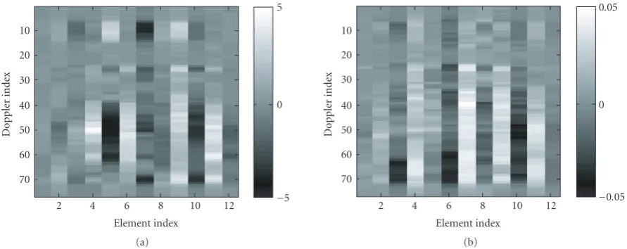
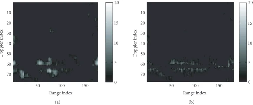
Figure 5shows the phase and log-amplitude errors as a function of Doppler filter and antenna channel that were calculated using the procedure described in the last section. Figure 6shows the effects of incorporating these corrections on the residual clutter-to-noise ratio (CNR) after KASTAP processing. This result shows that performing the adaptive gain/phase correction significantly reduces the amount of undernulled clutter, which in turn should reduce false alarms and improve detection performance. Figure 7 shows that performing eigenvalue rescaling further reduces the residual CNR after KASTAP processing.
70 60 50 40 30 20 10
Doppler
inde
x
2 4 6 8 10 12
Element index
−5 0 5
(a)
70 60 50 40 30 20 10
Doppler
inde
x
2 4 6 8 10 12
Element index
−0.05 0 0.05
(b)
Figure5: (a) Estimated phase and (b) long-amplitude errors as a function of Doppler filter (vertical) and antenna channel (horizontal).
70 60 50 40 30 20 10
Doppler
inde
x
50 100 150
Range index
0 5 10 15 20
(a)
70 60 50 40 30 20 10
Doppler
inde
x
50 100 150
Range index
0 5 10 15 20
(b)
Figure6: Residual CNR after KASTAP processing (a) without and (b) with corrections for channel- and Doppler-dependent gain and phase errors.
3.2. Detection/false alarm performance
In addition to SINR loss and residual CNR, performance was evaluated by processing the KASSPER data cubes with sim-ulated targets in them and comparing threshold crossings to the known target range/Doppler locations. Strong discretes and targets contaminate the training data and can cause se-vere nulling of target returns, thus reducing target detection performance. This contamination of the range-averaged co-variance estimates was reduced by performing separate range masking in each Doppler filter. To accomplish this, a two-step procedure was employed.
(1) Calculate the STAP detection statistic in each range/ Doppler cell without any masking of the training data (the detection statistic is determined by normalizing the output amplitudes so that the mean output noise power is at 0 dB and then performing a range-only CFAR in each Doppler fil-ter).
(2) Mask range/Doppler cells whose statistic exceeds a certain threshold (15 dB) from the training data. Recompute the detection statistic using the remaining training data and determine the resulting threshold crossings.
Figures9,10, and11 compare the range/Doppler loca-tions of threshold crossings in the same portion of CPI #22 as in Figures4–8. The locations of known targets are shown as diamonds for mainlobe targets and squares for sidelobe tar-gets. Threshold crossings due to targets are shown as light tri-angles, while false alarms are shown as light crosses. Observe that KASTAP produces fewer false alarms and more targets detections than standard STAP processing, especially when the adaptive gain/phase corrections and eigenvalue rescaling are performed (Figure 11).
70 60 50 40 30 20 10
Doppler
inde
x
50 100 150
Range index
0 5 10 15 20
(a)
70 60 50 40 30 20 10
Doppler
inde
x
50 100 150
Range index
0 5 10 15 20
(b)
Figure7: Residual CNR and KASTAP processing (with gain/phase correction) (a) without and (b) with eigenvalue rescaling.
70 60 50 40 30 20 10
Doppler
inde
x
50 100 150
Range gate
−40
−30
−20
−10 0
(a)
70 60 50 40 30 20 10
Doppler
inde
x
50 100 150
Range gate
−40
−30
−20
−10 0
(b)
Figure8: (a) SINR loss as a function of Doppler filter and range gate for standard STAP processing and (b) KASTAP processing with gain/phase correction and eigenvalue rescaling applied.
fraction of mainlobe targets that were detected within the range window processed. Multiple targets lying within the same range/Doppler cell were counted as a single target. For each threshold setting, the detection probability and false alarm density (number of alarms per square kilometer on the ground) were calculated. The range and azimuth extent pro-cessed corresponded to an area on the ground of 3 square kilometers per CPI.
Figure 12 shows the ROC curves representing perfor-mance over 29 CPIs of the KASSPER Data Set 2. A signifi-cant number of closely spaced, nonmoving targets were ac-tually present in the scenes. Since these targets are not mov-ing, their returns cannot be distinguished from those of clut-ter using Doppler frequency. Thus, even with KASTAP pro-cessing we cannot expect to achieve 100% detection proba-bility. A consistent benefit in detection performance is seen from KASTAP processing. For example, at a detection prob-ability of 60%, the false alarm density decreases from about 55 alarms per square kilometer for standard STAP process-ing to 1.5 per square kilometer for KASTAP processing (with
corrections and eigenvalue rescaling), a factor of more than 30 reduction. If the nonmovers were removed from the data set, the detection probability values obtained would be ex-pected to increase accordingly.
−70
−60
−50
−40
−30
−20
−10
Doppler
inde
x
0 50 100 150
Range index Truth (mainlobe)
Truth (sidelobe)
TGT crossings False alarms
Figure9: Range-Doppler locations of target truth (mainlobe and sidelobe targets), target threshold crossings, and false alarms for standard STAP processing on CPI #22 of the KASSPER Data Set 2.
−70
−60
−50
−40
−30
−20
−10
Doppler
inde
x
0 50 100 150
Range index Truth (mainlobe)
Truth (sidelobe)
TGT crossings False alarms
Figure 10: Range-Doppler locations of target truth (mainlobe sidelobe targets), target threshold crossings, and false alarms for KASTAP processing (without gain/phase correction or eigenvalue rescaling) on CPI #22 of the KASSPER Data Set 2.
4. MITIGATION OF LARGE DISCRETE RETURNS
The KASTAP techniques described in Sections2and3were developed for a radar interference environment consisting of strong, nonhomogeneous distributed clutter returns as well as numerous target returns. Real-world GMTI surveillance
−70
−60
−50
−40
−30
−20
−10
Doppler
inde
x
0 50 100 150
Range index Truth (mainlobe)
Truth (sidelobe)
TGT crossings False alarms
Figure11: Range-Doppler locations of target truth (mainlobe and sidelobe targets), target threshold crossings, and false alarms for KASTAP processing (with gain/phase correction and eigenvalue re-scaling) on CPI #22 of the KASSPER Data Set 2.
0 0.2 0.4 0.6 0.8 1
P
robabilit
y
o
f
d
et
ection
100 101 102
False alarm density (1/km2)
KASTAP (corr.)
KASTAP (no corr.)
Std. STAP
Figure12: ROC curves for standard STAP, KASTAP without cor-rections or eigenvalue rescaling, and KASTAP with corcor-rections and eigenvalue rescaling over 29 CPIs of the KASSPER Data Set 2.
Target 1
Target 2 Target 3
Target 4
Road network
∼820 m
(a)
Standard STAP KASTAP
Target#1 detections 12 22
Target#1 time in track 130 s 230 s
Target#2 detections 17 19
Target#2 time in track 230 s 230 s
Target#3 detections 17 21
Target#3 time in track 220 s 210.20 s∗
Target#4 detections 7 17
Target#4 time in track 60 s 210 s
False alarms 28 10
∗Two tracks formed on target (b)
Figure13: (a) Target locations on our DM++ display and (b) tracking results for standard-versus-KASTAP processing.
35.89 35.885 35.88
Latitude
(
◦)
−117.92 −117.91 −117.9 Longitude (◦)
−80
−60
−40
−20 0
(a)
0 0.2 0.4 0.6 0.8 1
P
robabilit
y
o
f
d
et
ection
100 101 102
False alarm density (km−2)
No discretes present
Discretes present
(b)
Figure14: (a) Effects of multiple discretes on CPI #22 clutter reflectivity estimates and (b) KASTAP ROC curves.
describe a set of techniques that we developed and incor-porated into our KASTAP processing to mitigate the effects of large clutter discretes. Finally, inSection 4.3we show the results of applying these techniques to the KASSPER Data Set 2.
4.1. Effect of large discretes on KASTAP performance
Though discrete returns from buildings and towers were sim-ulated in the KASSPER Data Set 2, the radar cross section (RCS) of these scatterers was limited by a fairly small build-ing size [9]. In urban regions, buildbuild-ings can have an RCS as high as 106m2[12]. In order to simulate the effects of
mul-tiple large discretes, we used the routines supplied with the KASSPER Data Set 2 [9] to add plane wave responses from 5 point scatterers located on visible terrain to the CPI #22 data cube. We set the radar cross section of the discretes to be 40 dB m2to represent the returns from moderately large
buildings.
Figure 14(a)shows that the effects of these discretes are clearly visible in the clutter reflectivity map estimates. Due to the fact that the discretes are not exactly located on one of the
point scattering locations in our distributed clutter model, they corrupt reflectivity estimates over a wide area through sidelobe effects. The covariance matrices derived from the clutter reflectivity map also rely on a point scattering model. In addition, the model errors estimated for distributed clut-ter may be inadequate for suppressing the discrete. Thus, while there will be some suppression of the discretes by the KASTAP filter weights, undernulling can be expected to oc-cur. With KASTAP processing, the discretes are found to pro-duce false alarms in many Doppler filters.Figure 14(b)shows that the KASTAP ROC curves for CPI #22 are highly de-graded by the presence of the discretes.
4.2. Suppression of discrete returns
We studied a number of different approaches for suppressing the effects of discretes on STAP performance. The technique we found to be most effective for suppressing the discrete re-turns comprises of 5 steps.
(2) Estimate the complex amplitude and azimuth angle of a discrete in each range gate containing threshold crossings fromStep 1.
(3) Subtract the estimated discrete contributions to clut-ter reflectivity estimates.
(4) Estimate channel-dependent gain and phase errors to apply to the space-time steering vectors at the discrete loca-tions using a maximum likelihood approach.
(5) Add an additional constraint on the STAP weight vec-tor to place a deterministic null on each discrete.
We describe each of these steps individually below.
Step 1(discrete detection). In this step, we detect the pres-ence of discretes on a given CPI using the clutter reflectivity estimates. These estimates are first computed as described in Section 2.1.3. As discussed there, space-time steering vectors
sito the clutter scatterersiin each range gate of a CPI data cube are first defined. The complex return strengths αiare then calculated as shown in (5). The thresholding process in a given range gate of a CPI data cube is then specified by
max i
αi2
> T. (23)
If the threshold is crossed, we proceed toStep 2 which estimates the complex amplitude and azimuth angle of the discrete. In addition, we exclude range gates in which dis-cretes are detected from the training data for the estimation of the distributed clutter gain and phase errors described in Section 2.3.3. This prevents the discretes from contaminating the model error terms applied to distributed clutter.
Step 2(discrete azimuth and amplitude estimation). In this step, to prepare for removing the effects of the discrete de-tected inStep 1, we perform a fine estimation of the discrete azimuth angle and its complex amplitude. A bank of space-time steering vectorssi,jis defined corresponding to a fine az-imuth spacing along the clutter ridge. Here,ilabels the clut-ter cell as inStep 1, and jis an oversample index specifying the azimuth angle within the clutter cell. We then determine the indices that maximize the following quantity:
id,jd
: max {i,j}si,j
Hx=s
id,jdHx. (24)
These indices define a maximum likelihood estimate of the discrete azimuth angle, assuming that the data vector con-tains only a single discrete return and additive noise. This as-sumption is based on the largeness of the discrete amplitude compared to distributed clutter returns. Under this model, the maximum likelihood estimate of the complex amplitude of the discrete is given by
αd=
sid,jdHx
sid,jdHsid,jd. (25)
Step 3(clutter reflectivity map correction). In order to elim-inate contamination of the clutter reflectivity estimates, dur-ing estimation of clutter reflectivity we modify the radar data vector as follows:
x−→x−αd·sid,jd. (26)
The complex amplitudes of each clutter scatterer are then re-estimated using (5). This effectively removes the contribu-tion of the discrete to the clutter reflectivity map. Rather than being incorporated into the knowledge-aided covariance, a deterministic nulling of the discrete will be performed as de-scribed inStep 5.
Step 4(discrete channel-dependent gain/phase error estima-tion). Though estimation of channel-dependent gain and phase errors in each Doppler filter is already being performed in our KASTAP processing, these terms will be incorrect when applied to the return from the discrete. This is due to the fact that the location of the strongest distributed clut-ter in each Doppler filclut-ter is different from the location of the discrete (due to the largeness of the discrete, it affects all Doppler filters through sidelobe effects). Thus, the channel-and angle-dependent antenna errors on the discrete will be different from that on distributed clutter. If we are in the Doppler filter in which the strongest distributed clutter is coming from the clutter cell containing the discrete, the dif-ferences will be much smaller. However, they will still be present and due to the strength of the discrete return, more accurate knowledge of the gain and phase errors at the dis-crete location is required to provide sufficient nulling.
To perform this step it was found beneficial to first perform KASTAP processing and obtain a KASTAP covari-ance estimateRCLusing the KASTAP approach we have
de-scribed in previous sections. This estimate is calculated for the Doppler filter containing the maximum amplitude from the discrete (determined by applying Doppler filter weights to sid,jd and looking for the filter with the maximum am-plitude). It describes the statistics of the distributed clutter returns in the range gate and Doppler filter containing the discrete. The adjacent-bin Doppler preprocessing matrix for this filter is then applied to the full-DOF data vectorxand the discrete steering vectorsid,jd, yielding a reduced-DOF data vectoryand a reduced-DOF discrete steering vectorsd, re-spectively.
A set ofN complex errors en,n = 1, 2,. . .,N, is next defined. These error terms define a modified, reduced-DOF discrete space-time steering vector whose elements are given by
s(corrd .)
n+(f−1)·N =
1 +en
·sd
n+(f−1)·N. (27)
Here, n is the antenna channel index and f is the adja-cent filter index for the adjaadja-cent-bin post-Doppler degrees algorithm. To determine the error terms, we model the reduced-DOF data vector y in the range gate containing the discrete as
y=αd·s(corrd .)+yc, (28)
whereycis a complex Gaussian random vector with covari-ance matrixRCL (representing the distributed clutter). The
35.89 35.885 35.88
Latitude
(
◦)
−117.92 −117.91 −117.9 Longitude (◦)
−80
−60
−40
−20 0
(a)
0 0.2 0.4 0.6 0.8 1
P
robabilit
y
o
f
d
et
ection
100 101 102
False alarm density (km−2)
KASTAP with discrete suppression
KASTAP without discrete suppression
(b)
Figure15: (a) Effects of discrete suppression processing on CPI #22 clutter reflectivity estimates and (b) KASTAP ROC curves.
maximize the log-likelihood function
lnpy|e= −y−αd·s(corrd .)
H
RCL−1
y−αd·s(corrd .)
− N
n=1 en2
σe2 + const.
(29)
Note that we have added a complex Gaussian prior distribu-tion onenwith varianceσe2. The variance is selected to be 1 in order to force the constraint that the errors are small. We next vary the log-likelihood function with respect to the real and imaginary parts ofen(or, equivalently, with respect toen anden∗). Remembering thats(corrd .)depends onenas shown above, equating the coefficients ofδeandδe∗to zero gives a linear set of equations for the error termsenwhich are readily solved.
Note that we have used a particular Doppler filter, the filter with the largest discrete amplitude contribution, to es-timate the channel-dependent gain error terms on the dis-crete. InStep 5we want to use this information to improve STAP performance inallthe Doppler filters. In order to do this, once the error terms are obtained, the corrected full-DOFspace-time steering vector for the discrete is calculated as
s(corrid,jd.)
n+(m−1)·N =
1 +en
·sid,jd
n+(m−1)·N. (30)
(Here,mis the pulse index ranging from 1 to the number of pulsesM.) InStep 5, we compute corrected reduced-DOF discrete steering vectors ineachDoppler filter by applying the appropriate Doppler preprocessing matrix to the corrected full-DOF steering vector shown above.
Step 5 (KASTAP filter weights with deterministic null on discrete). Given an estimated covariance RCL, the
“stan-dard” KASTAP weight vectorwKAis computed by
minimiz-ingwKAHRCLwKA subject to a gain constraint on the target
steering vectorst. This gives the familiar expression
wKA=β·RCL−1st. (31)
We modified this to apply, in addition to the target gain constraint, a null constraint on the corrected, reduced-DOF discrete steering vector. This is repeated ineachDoppler fil-ter, not just the filter containing the maximum discrete am-plitude, so that the sidelobe effects of the discrete can also be removed. In a given Doppler filter q, we define a cor-rected reduced-DOF steering vectors(dq,corr.)by applying the adjacent-bin preprocessing matrix for filterq to the vector
s(corrid,jd.)shown in (30).
Next, we solve the constrained minimization problem
min
wKA
wKAHRCLwKA s.t. wKAHst=1, wKAHs(dq,corr.)=0.
(32)
This can be solved using Lagrange multipliers, yielding
wKA=β·RCL−1
st−γ·s(dq,corr.)
,
γ= s
(q,corr.)H d RCL−1st
s(dq,corr.)HRCL−1s (q,corr.)
d
.
(33)
It is easily verified that this weight vector satisfies the null constraintwKAHs(dq,corr.) = 0. The constantβ is selected to
satisfy the target gain constraint (however, since it is only an overall scale factor, βhas no effect on the output SINR or CNR).
4.3. KASTAP results with discrete suppression processing
the “cleaning” procedure (Step 3of the procedure described in the last section) was effective in removing the large am-plitude contributions of the discrete to the clutter reflectiv-ity map. Figure 15(b)shows that all of the degradation in the ROC curve caused by the discretes has been eliminated through use of the discrete suppression algorithm described in the last section.
5. SUMMARY
We have described in this paper knowledge-aided STAP pro-cessing using multilook GMTI radar data. The algorithm reg-isters the data to an earth-based coordinate system and forms clutter reflectivity maps, which are used to calculate pre-dicted distributed clutter statistics. Adaptive incorporation of current-CPI data into the reflectivity maps is also performed to improve local reflectivity estimates when large changes oc-cur as the platform geometry evolves. The clutter reflectiv-ity map predictions are incorporated into robust STAP pro-cessing using a procedure that combines covariance taper-ing to account for ICM, adaptive correction for Doppler and channel-dependent gain and phase mismatch, knowledge-aided prewhitening, and eigenvalue rescaling. The effects of target contamination of the STAP training data are sup-pressed from the covariance estimates in each Doppler filter using masking of detections in a two-pass procedure. The ap-proach was applied to the KASSPER Data Set 2 and KASTAP performance characterized in terms of SINR loss, resid-ual CNR, target detections and false alarms, ROC curves, and track life. The results show improved detection of low-velocity targets and more than an order of magnitude reduc-tion in false alarm density compared to standard STAP pro-cessing. Additional techniques to detect and suppress large clutter discretes have been defined and shown to be effective in reducing the degradation in KASTAP performance caused by these discretes.
ACKNOWLEDGMENT
The authors would like to thank the Defense Advanced Re-search Projects Agency for funding this work under Contract F30602-02-C-0010.
REFERENCES
[1] W. L. Melvin, “Space-time adaptive radar performance in het-erogeneous clutter,”IEEE Transactions on Aerospace and Elec-tronic Systems, vol. 36, no. 2, pp. 621–633, 2000.
[2] W. L. Melvin, J. R. Guerci, M. J. Callahan, and M. C. Wicks, “Design of adaptive detection algorithms for surveillance radar,” inProceedings of Record of the IEEE 2000 International Radar Conference, pp. 608–613, Alexandria, Va, USA, May 2000.
[3] J. Ward, “Space-time adaptive processing for airborne radar,” Tech. Rep. F19628-95-C-0002, MIT Lincoln Laboratory, Lex-ington, Mass, USA, 1994.
[4] I. S. Reed, J. D. Mallett, and L. E. Brennan, “Rapid convergence rate in adaptive arrays,”IEEE Transactions on Aerospace and Electronic Systems, vol. 10, no. 6, pp. 853–863, 1974.
[5] J. R. Guerci, “Theory and application of covariance matrix ta-pers for robust adaptive beamforming,”IEEE Transactions on Signal Processing, vol. 47, no. 4, pp. 977–985, 1999.
[6] R. C. DiPietro, “Extended factored space-time processing for airborne radar systems,” inProceedings of 26th IEEE Asilomar Conference on Signals, Systems and Computers, vol. 1, pp. 425– 430, Pacific Grove, Calif, USA, October 1992.
[7] J. S. Bergin, J. R. Guerci, P. M. Techau, and C. M. Teix-eira, “Space-time beamforming with knowledge-aided con-straints,” inProceedings of 11th Workshop on Adaptive Sensor Array Processing (ASAP ’03), Lexington, Mass, USA, March 2003.
[8] J. S. Bergin, C. M. Teixeira, P. M. Techau, and J. R. Guerci, “STAP with knowledge-aided data pre-whitening,” in Proceed-ings of IEEE Radar Conference, pp. 289–294, Philadelphia, Pa, USA, April 2004.
[9] “High-Fidelity Site-Specific Radar Simulation: KASSPER Data Set 2,” Information Systems Laboratories, Inc., October 2002. [10] E. J. Kelly, “An adaptive detection algorithm,”IEEE Transac-tions on Aerospace and Electronic Systems, vol. 22, no. 1, pp. 115–127, 1986.
[11] L. Novak, “New results in UHF/VHF SAR change detection,” inCCC&D FOPEN Workshop, MIT Lincoln Laboratory, Lex-ington, Mass, USA, October 2002.
[12] M. I. Skolnik, Ed.,Radar Handbook, McGraw-Hill, New York, NY, USA, 2nd edition, 1990, Section 17.2.
Douglas Pagereceived the B.S. (1983) and M.Eng. (1984) degrees in electrical engineering, and the Ph.D. (1992) degree in physics from Rensselaer Polytechnic Institute. From 1993 to 2000, he was with Technology Service Corporation (TSC) in Trumbull, Conn, working on a variety of problems in radar simulation and algo-rithm development. This included developing and simulating the performance of space-time adaptive processing (STAP) algorithms. From April 2000 through October 2002, Dr. Page was with the MITRE Corporation in Bedford, Mass, where he continued work in radar signal processing, including target detection in synthetic aperture radar (SAR) imagery. He joined BAE Systems in Novem-ber 2002, where he has been developing STAP techniques in con-nection with several different programs. Dr. Page is a Member of the Tau Beta Pi, Eta Kappa Nu, and Signal Xi Honor Societies.