Improving the Performance and Sensitivity of Gravitational Wave Detectors

(1)

Wave Detectors

Thesis by

Eric Antonio Quintero

In Partial Fulfillment of the Requirements for the degree of

Doctor of Philosophy

CALIFORNIA INSTITUTE OF TECHNOLOGY Pasadena, California

2018

(2)

Eric Antonio Quintero ORCID: 0000-0002-4269-3445

(3)

Acknowledgements

My time at Caltech has benefitted immensely from those who have supported and accom-panied me. These words are a poor renumeration for this service; my sincere gratitude goes out to all those with whom I have crossed paths over these years.

I could hardly have conceived of taking this path were it not for the relentless support and encouragement of my parents and grandparents, tireless champions for my academic pur-suits and passions. My sister was also a reliable trail-blazer and companion, from reading stories to reading thesis drafts. I hope to deserve their efforts by paying it forward.

It has been a distinct privilege to be part of the LIGO Scientific Collaboration and LIGO Laboratory; witnessing groundbreaking discoveries first-hand, along with the years of tireless work that brought these to fruition. I continue to be astounded by the dedication and ability of those I am fortunate enough to call colleagues, including M. Abernathy, A. Brooks, C. Cahillane, T. Chalermsongsak, K. Dooley, J. Eichholz, E. Gustafson, E. Hall, J. Kanner, Z. Korth, H. Miao, X. Ni, N. Robertson, J. Smith, M. Thirugnanasambandam, S. Vass, G. Venugopalan, A. Wade, and H. Yamamoto. I would particularly like to thank those who I have come to consider mentors of one form or another who have taught me so much, both professionally and personally: K. Arai, J. Driggers, J. Rollins, N. Smith, R. Smith, G. Vajente, S. Waldman, and D. Yeaton-Massey. I thank my advisor, R. X. Adhikari, for helping me learn from the past, helping me see what matters, and showing me how to be a scientist.

My deepest thanks to the friends who tolerated my madness throughout these years. A shout-out to those who hail from the dark side: D. Bickerstaff, L. Tenorio, J. Motes, K. Rose (plus little K and H!). Thanks to J. Duarte and I. Saberi for sharing the road, some roofs, and some Ernie’s.

(4)

Abstract

The field of observational gravitational wave astronomy has begun in earnest, starting with the detection of the strain signal from the binary black hole merger GW150914 by the Laser Interferometer Gravitational-wave Observatory (LIGO) in 2015. The current incarnation of the LIGO observatories, known as Advanced LIGO, has achieved strain sensitivities on the order of 10−23/√Hz in the hundreds of Hz region, which has en-abled unambiguous detection of astrophysical gravitational wave signals. Nevertheless, the scientific output from the LIGO observatories is constrained by the instrumental performance and sensitivity, as there remain many more distant and exotic sources to be observed.

This thesis describes a few topics in experimental gravitational physics, broadly unified by the desire to improve the performance and sensitivity of gravitational wave interfer-ometers. First, it describes an experimental effort to search for a novel form of nonlinear mechanical noise that may be relevant for the ultimate performance of the mirror sus-pension systems used throughout the instrument. Next, it summarizes work done at the CalTech 40m LIGO controls prototype to realize its fully operational state, and a novel automated controls algorithm developed and tested there that may be useful in simpli-fying the control of current and future interferometers. Finally, it describes work done on a system to identify and subtract unwanted noise couplings out of recorded aLIGO strain data in an automated fashion. The noise subtraction system applied to GW150914 is demonstrated to reduce the uncertainties of the black hole mass parameters by about 10 %.

(5)

Published Content and

Contributions

Chapter2is adapted from Vajente, Quintero, et al. [1]. E. A. Quintero performed the construction and characterization of the initial measurement prototype, developed the demodulation analysis, assisted in the conceptual design and assembly of the improved measurement system, and contributed to the writing of the manuscript for publication.

(6)

LIST OF ILLUSTRATIONS

Number Page

1.1 Michelson Interferometer . . . 5

1.2 Schematic of aLIGO DRSE optical configuration . . . 8

1.3 Angular cavity modes modified by radiation pressure torque . . . 10

1.4 Schematic representation of the ALS subsystem . . . 14

2.1 aLIGO Quadruple Pendulum Test Mass Suspension . . . 19

2.2 Schematic of Michelson Interferometer blade motion measurement . . . 21

2.3 Qualitative illustration of up-conversion noise signals . . . 26

2.4 Simulated results of non-linear noise demodulation analysis . . . 27

2.5 Loaded test blade assembly . . . 30

2.6 Prototype Noise Budget . . . 31

2.7 Limits of nonlinear noise in aLIGO blade springs from prototype exper-iment.. . . 31

2.8 Rendering of improved measurement apparatus . . . 33

2.9 Optical schematic of improved apparatus . . . 34

2.10 Seismic isolation system of the improved apparatus. . . 37

2.11 Noise performance of the improved apparatus . . . 38

3.1 Schematic of 40m Length Sensing System . . . 46

3.2 ALS Sensitivity Improvement . . . 48

3.3 Effects of PRC Angular Feed-forward . . . 50

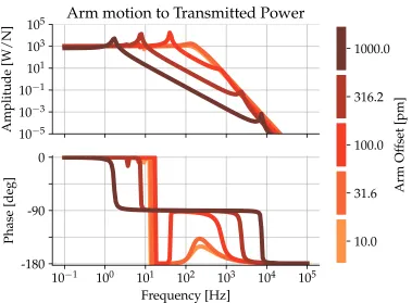
3.4 Simulated response of IR transmitted light signals to CARM fluctuations at the 40m prototype . . . 52

3.5 Frequency dependent CARM error signal blending . . . 54

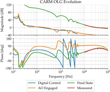
3.6 CARM open loop gain at different stages of lock acquisition . . . 55

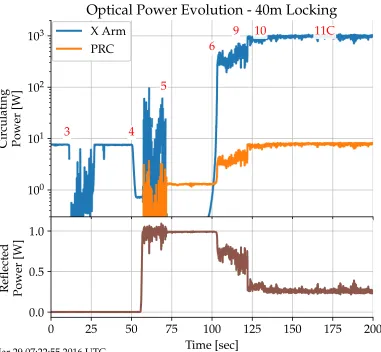
3.7 Evolution of Circulating Power during Lock Acquisition . . . 56

3.8 Error Signal Blending During Lock Acquisition . . . 57

3.9 40m Prototype Fundamental Noises . . . 62

3.10 Achieved displacement sensitivity of the 40m prototype interferometer . 63 3.11 40m DRFPMI Sensing Matrix . . . 64

3.12 AS port camera during DRFPMI Lock . . . 65

3.13 REFL port during DRFPMI Lock . . . 65

(8)

3.15 Signal Recylcing vs. Signal Extraction for the 40m Prototype . . . 68

4.1 Feedback topology considered for the CESAR algorithm . . . 74

4.2 40m Arm Cavity Signals . . . 81

4.3 Time Domain Simulation of a Fabry-Pérot cavity scan using the CESAR algorithm . . . 84

4.4 IR Lock acquisition of a 40m arm cavity using the CESAR algorithm . . 85

5.1 Representative O1 aLIGO Noise at Low Frequencies . . . 88

5.2 Simple additive signal model . . . 92

5.3 Results of Greedy Ranking Search for H1. . . 103

5.4 Results of Greedy Ranking Search for L1 . . . 104

5.5 PSDs of H1 Wiener Filter Validation around GW150914 . . . 105

5.6 PSDs of L1 Wiener Filter Validation around GW150914 . . . 106

5.7 Comparison of Hardware Injection Posteriors . . . 107

5.8 Comparison of Filtered GW150914 Timeseries . . . 109

5.9 Improvement of GW150914 Mass Posteriors . . . 110

5.10 Improvement of GW150914 Final Black Hole Parameters . . . 111

5.11 ASDs of mock nonlinear noises . . . 115

5.12 Schematic of nonlinear regression ANN . . . 116

5.13 Neural Network Learning Loss . . . 118

5.14 Regression of mocked bilinear Noise . . . 119

(9)

LIST OF TABLES

Number Page

1.1 Summary of desired interferometric conditions for the aLIGO DRSE

scheme. . . 11

1.2 Summary of optical heterodyne signals used for steady-state interfero-metric length sensing in aLIGO [13,15] . . . 12

1.3 Summary of optical heterodyne signals used for the third harmonic de-modulation technique in aLIGO . . . 15

3.1 Comparison of aLIGO and 40m Prototype Parameters . . . 43

3.2 Sensors used for Interferometer Length Controls . . . 45

5.1 Time intervals used for GW150914 noise subtraction analysis . . . 101

5.2 Channels identified by the greedy ranking algorithm. . . 102

(10)

Chapter 1

Introduction

Einstein’s theory of General Relativity is our current best understanding of the physics of extremely massive objects. [1] The defining characteristic of General Relativity is the con-cept that gravitation can be understood as the fundamentally geometric effect of space-time curvature. According to Misner et al. [2], “space-time tells matter how to move; matter tells space-time how to curve.” Furthermore, Einstein found that his theory sup-ported wave solutions in the linearised weak-field regime[3], though there was debate over their physical reality and skepticism concerning the feasibility of their detection.

On human scales, however, space-time is extremely stiff. Our only means of investigating systems massive enough to exhibit strongly relativistic behavior is through the observa-tions of astrophysical systems. The Advanced LIGO (aLIGO) observatories[4], located in Hanford, WA and Livingston, LA, were constructed with the goal of observing gravi-tational waves of astrophysical origin, especially those arising from the dynamics of black holes and neutron stars.

Operating at a space-time strain sensitivity on the order of 10−23/√Hz during their first observing run [5], the aLIGO observatories made the first direct observation of gravita-tional waves [6], from the merger of two black holes. This discovery has begun the era of gravitational wave astronomy, which will enable many new kinds of observations that will inform and expand our understanding of the universe.

(11)

1.1

Gravitational Waves in General Relativity

The metric tensorgµν, or simply the metric, is a fundamental quantity of space-time in General Relativity, as it allows us to quantify intervals in space and time as we measure them, viads2 = gµνdxµdxν. To find the metric for a given configuration of matter and energy defined by the stress-energy tensorTµν, one must solve the Einstein field equation:

Gµν = 8_cπ₄Tµν (1.1)

Here,Gµν is the Einstein tensor, which is a compact tensor representation of space-time curvature and a function of the metric.

Distant from any massive objects,Tµν ≈ _{0, and the space-time curvature is small. In this} weak-field limit, we may solve the Einstein field equation to find that the metric can be written as

gµν ≈ ηµν +hµν (1.2)

whereηµνis the Minkowski metric of flat space-time, andhµν is a small perturbation of much smaller magnitude. In the transverse-traceless gauge, hµν can be understood as a strainin space-time itself, causing a relative change in the distance between two points in space-time.

In this weak field limit, it can be shown that the following wave equation holds forhµν[2]:

∇2− 1 c2

∂2

∂t2

hµν = 0 (1.3)

Thus, empty space-time can supportgravitational waves, transverse fluctuations of the space-time metric that propagate atc. Plane wave solutions to the wave equation travel-ing along thezaxis can be written in the transverse traceless gauge as:

hµν(z,t)=          

0 0 0 0

0 −h₊ h× ₀ 0 h× h+ 0

0 0 0 0

         

sin ω(t− _cz)

(1.4)

where h+ and h× are the two possible orthogonal polarizations, and ω is the angular frequency of the wave.

The simplest conditions necessary for the generation of gravitational waves is a time-varying mass quadrupole moment [7]:

hµν(t,r)= 2G

rc4IµνÜ (t− r

(12)

For instance, a pair of point masses in circular orbit about their common center of mass with constant orbital frequencyωohas a quadrupole moment with terms proportional to sin2(ω_ot)_{. This in turn causes the emission of gravitational waves at a frequency of} 2ωo.

(13)

1.2

Making Gravitational Waves Observable

In order to record a gravitational wave signal with some scientific apparatus, the wave must be transduced into some physical quantity that is more conveniently measured. One of the threads of thought that contributed to the early conceptions of LIGO was that a gravitational wave would affect the time of flight of light traveling between two freely falling test masses. Following the derivation in Saulson [7], let us consider an incident sinusoidal plane wave in the+polarization with angular frequencyωGW, am-plitudeh, and wave vectork= ωGW

c ˆz. Since light follows trajectories satisfyingds2 =0, the time to travel a distanceLalong thex-axis in the transverse-traceless gauge is, to first order inh:

τ=_c1

∫ L

0

dx√g_x,_x (1.6)

≈1 c

∫ L

0

dx 1+ ₂1hcos(ω_GWt)

(1.7)

=τ0

1+ hc

2 sinc(ωGWτ0)

(1.8)

whereτ0 B L_c is the travel time absent a gravitational wave. A ray of light simultane-ously propagating along they-axis will experience a similar shift in travel time due to the gravitational wave, but with opposite sign, sincehx,x = −hy,y. Thus, the two rays will experience adifferentialphase shift due to the incident gravitational wave.

Given this differential character, the perpendicular arms of a Michelson laser interferom-eter (see Figure1.1) lend themselves naturally to the transduction of a gravitational waves, as the recombination of the beams that have traveled to the end mirrors and back con-verts the phase shift into intensity fluctuations at the output (a.k.a. anti-symmetric) port of the interferometer.

In this case, the resultant difference in the light travel times corresponds to a differential phase shift according to:

∆φ(t)= 2πc

λ τ0sinc(ωGWτ0)hcos(ωGWt) (1.9) This phase shift changes the interference condition of the recombined beams at the out-put of the interferometer. If the interferometer is illuminated with a plane wave

Ein= E0ei 2πc

λ t _(1.10)

The power at the output of the interferometer follows

PAS = E2

in

(14)

L Laser

PD

Figure 1.1: Schematic representation of a Michelson interferometer for the transduction of gravitational waves to light intensity at the interferometer output. Laser light of wave-lengthλis incident on a beam-splitter, which sends half of the power down the two per-pendicular arms of lengthL. The light reflects off of the end mirrors, and recombines at the beam-splitter. Any differential phase shift experienced by the light while in the arms will manifest as a change in the interference condition at the output.

Thus, the Michelson interferometer gives us a means of transducing gravitational waves into optical power fluctuations, which are readily measurable. Furthermore, this is con-ceptually similar to how Michelson interferometers are used for measurements of dif-ferential length fluctuations of its arms via∆φ = 2_λπ∆LThus, the apparent differential length change due to an incident gravitational wave follows

∆L(t)= L_sinc(ω_GWτ₀)h_cos(ω_GWt) _(1.12)

These expressions can be simplified if we assume thatωGWτ0 1, which physically means that the metric perturbation is effectively constant during the time any given wave-front is propagating up and down an arm. Then, sinc(ω_GWτ₀) ≈ _{1 and we recover a} simple linear transduction of

∆L(t)

L = h(t) (1.13)

which reinforces the conception of a gravitational wave manifesting as space-time strain.

(15)

(16)

1.3

Gravitational Wave Interferometer Design

We will now briefly examine the optical configuration and the control systems necessary to operate the aLIGO interferometers. We will make several simplifications, as a complete description is beyond the scope of this work. For fuller treatments, see Aasi et al. [4], Mizuno et al. [9], Ward [10], Adhikari [11], Staley et al. [12], Martynov [13], Hall [14], and Izumi and Sigg [15].

1.3.1

Enhancing Interferometer Sensitivity with Resonant

Cavities

One way to enhance the response of a gravitational wave interferometer would be to use resonant Fabry-Pérot cavities in place of the long baseline Michelson arms. The resonant cavity effectively provides a greater phase response to length fluctuations that a Michelson arm, due to the increased light buildup and storage time. This does, however, decrease the response bandwidth of the interferometer.

However, there are still several practical drawbacks. Even if one separates the light re-flected back through the input (symmetric) port via polarization rotation or Faraday iso-lators to prevent illumination of the laser light source, one is effectively wasting a substan-tial amount of energy in light that carries a gravitational wave signal. One solution is to introduce an additional resonant cavity through the introduction of a partially transmis-sive mirror before the beamsplitter, referred to aspower recycling. Furthermore, one can arrange the differential distance of the input test masses from the beamsplitter to operate on the dark fringe of the Michelson, thereby resonating the maximum available power in the power recycling cavity (PRC). This can greatly increase the power buildup in the arm cavities, further enhancing the sensitivity; this was the basic configuration of the initial iterations of LIGO [16].

A practical drawback of increasing the light power stored in the arm cavities via increased finesse and power recycling gain is the narrowing of the interferometer bandwidth; while the low frequency response is enhanced, the interferometer loses the ability to sense high frequency sources. Since there are many technical noise sources at low frequencies that limit the utility of sensitivity gains in that band, it is desirable to broaden the frequency response of the instrument without reducing the power stored in the arms.

(17)

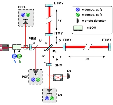
LIGO-T1500461–v3

lp'

lx ly

9 MHz45 MHz

ri, ti re

rp, tp

rs, ts

ls' REFL

POP

AS

= demod. at 9 MHz = demod. at 45 MHz = photo detector

= EOM Ly

Lx

Figure 6: A schematic of the aLIGO interferometer setup.

A

Definitions and setup

A.1 Length degrees of freedom

We define the length DOFs as follows,

DARM: L = Lx Ly 2 , CARM: L+=

Lx+Ly

2 , PRCL: lp=l0p+

lx+ly

2 , MICH: l =lx ly

2 , SRCL: ls=l0s+

lx+ly

2 .

(37)

The optical distances are graphically shown in figure6.

page 23 LIGO-T1500325–v3

lp'

lx ly

9 MHz45 MHz

ri, ti re

rp, tp

rs, ts ls'

REFL

POP AS

= demod. at 9 MHz = demod. at 45 MHz

= photo detector

= EOM Ly

Lx

Figure 2: A schematic of the aLIGO interferometer setup. 2.2 Interferometric properties

We characterize the arm cavities by defining their reflectivities because we are always inter-ested in the fields in reflection rather than that in transmission. We write the amplitude reflectivity as,

ra⌘

re(t2i +ri2) ri 1 rire

, rˆa⌘

re(t2i +ri2) +ri 1 +rire

, (2)

where the first one denotes the reflectivity for the carrier light which is resonant and the other for the rf sidebands which are assumed to be exact anti-resonant. Note that we use a sign convention such that the reflectivity for the carrierra is positive for an over-coupled cavity, as opposed to that of the previous study [1]. Additionally, the interferometric conditions for the carrier and rf sideband fields are summarized in table1.

page 5 SRM PRM ITMY ITMX ETMY ETMX BS f1 f2 f2 f1

Figure 1.2: Schematic representation of the aLIGO DRSE optical configuration, includ-ing the output mode cleaner (OMC). Adapted from Izumi and Sigg [17].

(18)

1.3.2

Angular Cavity Dynamics

The test masses are subject to torque from the radiation pressure of the resonant field depending on the spot position, and the resultant angular motion will move the spot position in turn. Working out the dynamics of this system, two orthogonal modes of radiation pressure induced cavity tilt are evident for each angular degree of freedom (pitch and yaw): a “hard” and “soft” mode [19] (see Figure1.3). While the hard mode exerts a restoring torque, the soft mode on its own is unstable. When the soft mode’s radiation pressure angular spring constant exceeds that of the restoring mechanical spring constant of the mirror suspensions, the angular motion of the cavity mirrors becomes unstable. This occurs at the power given by:

P = κc_2L(1−_λ g)

a (1.14)

whereκis the mechanical angular spring constant,cis the speed of light,gis the cavity g-factor,Lis the cavity length andλais the soft mode eigenvalue of the transformation from pitch and yaw into the hard and soft angular modes.

1.3.3

Interferometric Length Sensing

It is generally necessary to use active feedback control to maintain the desired resonant operating condition in the interferometer, a complex affair due to the existence of mul-tiple degrees of freedom. Modulating the phase of the input laser light field provides a manner of measuring the relative phase shifts of different field components, which in turn carry information about the dynamics of the interferometer lengths. By detecting and demodulating the light fields at various points in the interferometer, it is possible to obtain linear feedback signals for the necessary degrees of freedom.

(19)

Figure 5-1. Illustration of the orthogonal modes of cavity tilt. The upper diagram shows tilts

given by eigenvector

⌥

v

_b

and the lower diagram shows

⌥

v

a

.

displacement

a

and cavity axis tilt

is also calculated for each eigenmode using the geometric

relationship between a set of mirror tilts and their cavity axis as derived in Appendix

C.2

. Figure

5-1

illustrates a cavity in each of the two eigenmodes when using the parameters from Table

5-1

.

5.1.2 Soft and Hard Modes

The torque to angle transfer function of each of these eigenmodes has the same form as that

of a single pendulum (Eq.

4–8

), but the torsion constant is modified. More importantly, the spring

constant is modified differently for each mode, yielding distinct behaviors of the two eigenmodes.

In this section, we analyze these behaviors and accordingly introduce the names

soft

and

hard

to

use in place of

a

and

b

for describing the two modes.

84

Figure 1.3: Depiction of the common and differential angular cavity motion mode, whose stiffnesses are modified by the torque induced by radiation pressure. Adapted from Doo-ley [19].

and the short Michelson differential displacement (MICH). These are defined as follows:

DARM:L−≡ Lx−Ly

2 (1.15)

CARM:L+≡ Lx+Ly 2

PRCL:lp ≡l0p+ lx+ly

2

SRCL:ls ≡ls0+ lx+ly

2

MICH:l− ≡lx−ly 2

(20)

as convenient). In aLIGO, f1 is approximately 9 MHz and f2 ≡ 5f1, which was chosen to be an exact multiple so that one RF oscillator can serve to synthesize all of the neces-sary signals. The desired interferometric conditions for the carrier field and the first order sideband fields is shown in Table1.1, which is achieved through the choice of macroscopic cavity lengths that create the desired free spectral range and resonance spectrum.

Table 1.1: Summary of desired interferometric conditions for the aLIGO DRSE scheme.

Frequency Offset [Hz] Arm Cavity PRC SRC

0 (Carrier) Resonant Resonant Anti-resonant

±f₁ Off Resonance Resonant Anti-resonant

±f₂ _{Off Resonance} _Resonant _Resonant

In addition to these resonance conditions, the MICH degree of freedom is held at the dark fringe condition, as mentioned previously. Nominally, this would not allow for any light to be present inside of the signal recycling cavity, rendering signal extraction inoperable. For this reason, a small asymmetry is introduced betweenlx andly, a.k.a./ the Schnupp Asymmetry. This breaks the clean separation between the common and differential vertex signals, but seeds the necessary resonating f2 fields in the SRC, and additionally allows for the sensing of SRCL and MICH signals at the reflected port.

When a cavity length fluctuates at a particular audio frequency, audio frequency side-bands are imparted onto any resonating or reflected carrier or sideband fields — the am-plitude of which depends on the resonance condition for that particular field. Optical beats between various fields can be demodulated to recover the audio frequency signal encoded upon them, as with the common Pound-Drever-Hall cavity stabilization tech-nique [20]. Roughly, we seek to demodulate components of optical beats that look some-thing like [15,21]:

Si =

∂E

a

∂Li ⊗Eb+Ea⊗

∂E_b

∂Li

∆L_iei(ωa−ωb)t _(1.16)

(21)

in-phase (I) and quadrature (Q), such that two degrees of freedom can be derived from one optical heterodyne beat. The sampled ports include the reflected field (REFL), the power-recycling cavity pick-off field (POP) and the output field at the anti-symmetric port (AS).

Table 1.2: Summary of optical heterodyne signals used for steady-state interferometric length sensing in aLIGO [13,15]

Length Port, Demod. Frequency Field Products

DARM ASf2 dECarrier ⊗E±f2

CARM REFLf1 dECarrier ⊗E±f1

PRCL POPf1 dECarrier⊗ E±f1,ECarrier⊗dE±f1

SRCL POPf2 ECarrier ⊗dE±f2

MICH POPf2 ECarrier ⊗dE±f2

Izumi and Sigg [15] describe the dependence of all of the RF photodetector responses to the various length degrees of freedom for the aLIGO interferometers. The ports and demodulation frequencies for the optical heterodyne readout of the length degrees of freedom is shown in Table1.2. In practice, signals from the AS port are only used to measure and control DARM, in part because it would be undesirable to have any com-peting feedback effects from other length control loops. All of the other length degrees of freedom have their length signals derived from the REFL and POP sensors. While the CARM signal generally dominates the content of the REFL and POP signals, using high-bandwidth analog laser frequency control suppresses the CARM influence on the residual POP and REFL signals, allowing for their use to control the DRMI.

Another enhancement designed for aLIGO was the use of an output mode cleaner at the anti-symmetric port, a ring cavity that only transmits the fundamental spatial mode of the carrier field, which is allowed to leak into the SRC and out of the AS port via a small DARM offset. This offset creates a first order coupling of DARM fluctuation to DC power transmitted through the OMC and providing a low noise strain signal, as the OMC rejects unwanted noise couplings due to higher order spatial modes and phase noise of the phase modulation oscillator.

(22)

operat-ing point. The mirror suspensions themselves are equipped with electromagnetic and/or electrostatic actuators which adjust the mirror position. The input laser frequency is also actively stabilized to the CARM degree of freedom by adjusting the error point of the laser’s frequency stabilization system via an additive offset (AO); this in turn uses a com-bination of broadband phase modulation, and adjustment of the input mode cleaner length.

Apart from the interferometric length stabilization loops, there are hundreds of auxil-iary control loops that are necessary for the optimal operation of the detectors, including thermal control of the test mass optics, angular control of the suspended optics, the active seismic isolation platforms, the laser frequency control, and more. This is all coordinate through a real-time digital control system, in which signals are digitized, user defined logic is applied to the signals, and actuation signals are synthesized and sent to actuators. The digital nature of this system allows for complex and interconnected logic between the var-ious subsystems. The majority of the real-time control system operates at a sampling rate of 16 384 Hz, which in practice affords digital control loops with control bandwidths of up to 100–200 Hz.

1.3.4

Advanced LIGO Locking

As will be discussed in some more detail in Section4.1, bringing the interferometer to its operating point — where all cavities are at the desired resonant condition and all the length degrees of freedom are under stable feedback control — is a very nontrivial af-fair, as the various cavities interact with each other in complex nonlinear ways. Here we will briefly describe two strategies employed in aLIGO that make the locking acquisition process more deterministic. Substantial information about development of the aLIGO locking procedures can be found in Staley et al. [12] and Martynov [13].

The primary complication that these strategies seek to simplify is the separation of initial control of the arm cavities and the DRMI cavities. The effective reflectivity of the arm cavities for the carrier light changes dramatically if the arm is flashing in and out of reso-nance, which makes the usual optical heterodyne signal unsuitable for stable control, as they depend directly on the carrier field amplitude (see Table1.2).

Arm Length Stabilization

(23)

auxil-14 ACQUISITION

DRMI Arm cavity (locked to arm)AUX laser

Offset Frequency discriminator Servo filter SHG SHG Beam splitter PD Dichroic Dichroic Main laser 0 a

Figure 3.6: Schematic view of the multi-color interferometry setup for arm length stabilisation.

An advantage in the use of this multi-color technique is that it provides signals with a substantially wide linear range with respect to the arm length. Thus the active control can be immediately engaged without fail. Moreover it can control the arm lengths such that the arm cavities are optically decoupled from the rest of the interferometer because of the wide linear range. As a consequent it avoids obstructions in the DRMI signals. On the other hand, one drawback is that this technique requires a large number of additional hardwares such as electronics, mirrors and lasers.

Recently the technique has been chosen to be a standard technique for lock acquisition in aLIGO and KAGRA. Although the working principle of

the ALS technique has been demonstrated by Mullavey et. al [12] in a

short-baseline cavity, the ALS technique needed further tests in a more realistic

configuration, which are summarized in chapter 5. Moreover the most

im-portant verification is the feasibility check — the noise performance must

satisfy the requirement for aLIGO. This is summarized in chapter 6.

This section describes the working principle of the ALS technique. The system can be divided into three subsystems and each of them is explained

in sections 3.4.2, 3.4.3 and 3.4.4 respectively. Then the requirements are

discussed in section 3.4.5.

3.4.2

Auxiliary Lasers for Sensing the Arm Length

To provide another sensor for the arm lengths, frequency-doubled Nd:YAG

(Nd-doped Y3Al5O12) lasers are introduced via second-harmonic generation

82

Figure 1.4: Schematic representation of the ALS subsystem. The green PDH locking components and second arm cavity are excluded for simplicity. Adapted from Izumi [24].

iary IR lasers that is PDH frequency locked to a single arm cavity to derive a cavity length signal that is independent from the main IR laser light that is present in the DRMI and subject to complex cavity couplings. A dichroic mirror coating on the test masses creates a lower finesse cavity for the green light. The transmitted green light is then interfered with frequency doubled light derived from the main input laser, as shown in Figure1.4.

Because of the PDH frequency locking, the green light frequency follows the free swing-ing arm cavity motion within the PDH control bandwidth. Then, the optical beat be-tween main laser green light and transmitted green light, which can be measured with a phase locked loop, carries information regarding the relative motion between the arm cavity and the input laser frequency, which in turn can be used as a new error signal to stabilize the arm cavity length with respect to the main laser frequency.

(24)

Third Harmonic Demodulation Technique

In order to reduce the influence of carrier light fluctuation, Arai [25] showed that one could derive signals from the optical beat at three times the modulation frequencies. While we usually only consider the first order sidebands that result from phase modu-lation, there are in reality many higher order PM sidebands that result, albeit with much reduced magnitude. Due to the FSR of the cavities, the second order PM sidebands can be used as stable local oscillators that will not interact with the cavities, and thereby pro-vide a consistent field product that only depends on the interaction of the first-order side-band fields with the DRMI. (See Table1.3) In truth, the sensitivity of these signals to the carrier is not zero, but the influence is reduced enough that the DRMI may be maintained stably on resonance regardless of the state of carrier light in the arm cavities.

Table 1.3: Summary of optical heterodyne signals used for the third harmonic demodu-lation technique in aLIGO

Length Port, Demod. Frequency Field Products

PRCL REFL 3f1 dE±f1⊗ E∓2f1

SRCL REFL 3f2 dE±f2 ⊗ E∓2f2

MICH REFL 3f2 dE±f2 ⊗ E∓2f2

aLIGO Lock Acquisition Sequence

Ideally, one could acquire control of the arm cavities with the ALS system, acquire con-trol of the DRMI with the 3f signals, and directly transition from ALS to IR optical heterodyne signals on resonance. Unfortunately, in part due to the dichroic mirror coat-ings for the ETMs currently not meeting their specification, it is necessary to slowly ap-proach resonance while the arms are under ALS control and use an intermediate IR sig-nal, as the residual cavity fluctuations while using ALS are wider than the interferometer linewidth [12].

Thus, the aLIGO locking procedure proceeds as follows:

1. The auxiliary lasers at each end station are frequency locked to the arm cavities via PDH reflection locking of the green light.

(25)

linewidths is introduced in the CARM control to avoid IR resonance of the main laser light.

3. Control of the DRMI is acquired using the 3f length signals.

4. The CARM offset is reduced to an intermediate point, where some IR light begins to resonate in the arm cavities.

5. CARM control is transitioned to use the DC power transmission through the arms as an error signal.

6. DARM control is transitioned to the ASf2RF optical heterodyne signal.

7. The CARM offset is further reduced until the REFLf1is viable, upon which it is used as the error signal, and the CARM offset is reduced to zero.

8. The interferometer is now fully resonating and is now transitioned to the lower noise DRMI length signals from the 1f POP RFPDs.

(26)

Chapter 2

Nonlinear Noise in Terrestrial

GW Detector Suspensions

2.1

Background

(27)

events at the test mass are small, their combined influence can introduce background noise which could limit the interferometer sensitivity.

Metals can also exhibit creep noise [30]. Although the underlying micro-mechanics of mechanical up-conversion and creep may be related, creep has a event rate that decreases quickly after the initial stress, and experimental investigations have shown that the creep can be reduced with the use of maraging steel [31–34]. Our experiment however focuses on mechanical events that are continuously triggered by a time varying external pertur-bation, such as the Advanced LIGO suspension cantilevers are subjected to by the local micro-seismic activity of the ground. In addition, since it is virtually impossible to distin-guish between events happening in the cantilevers from those happening in the suspen-sion wires or in the clamps, our system mimics as close as possible the Advanced LIGO configuration for cantilevers, wires and clamps.

It is known that crackling noise occurs when metals are stressed in the plastic regime. In the Advanced LIGO suspensions, however, the cantilever and wires loads are solidly within the macroscopically elastic regime, specifically≈_{50 % of the yield stress [}₂₈_{]. To} the best of our knowledge, there has been no in-depth investigation for potential discrete, stochastic deviation from linear mechanical behavior in crystalline materials this far be-low the engineering yield stress. Nevertheless, we can borrow insights from the existing experiments and theories which have studied the problem in the plastic regime. First of all, micro-pillar compression tests have demonstrated the dependence of event size on the driving mode: under load-controlled mode large bursts are seen, while displacement-controlled mode leads to slipping events of smaller sizes [35]. It has also been shown that the distribution of the size of crackling events depends on the stress and stress rate [36], being skewed toward smaller sizes for lower external stress and stress rate. These predic-tions have only been experimentally validated in the plastic regime, where burst sizes are large enough to exceed instrumental noises. Thus, the question of the existence of non-linear mechanical noise in the elastic regime remains open. Furthermore, the non-non-linear mechanical noise we are trying to characterize in the elastic regime — which we will here-after refer to asup-conversion noise— can have intrinsically different physical origins from the crackling noise studied in the plastic regime.

(28)

depend-Figure 2.1: The aLIGO test mass suspension system consists of a quadruple pendulum in-corporating 3 stages of maraging steel cantilever springs. Drawing adapted from Aston et al. [26].

(29)

2.2

Measurement method

A direct measurement of the horizontal displacement noise introduced by up-conversion events in the Advanced LIGO suspension cantilevers would be impossible except with an apparatus which has the same displacement sensitivity as the Advanced LIGO interfer-ometers [4]. However, any up-conversion noise at the level of the UIM cantilever springs will be attenuated by the additional vertical isolation provided by the lower suspension stages and by the relatively small coupling of vertical to horizontal test mass motion. For this reason, the sensitivity of our apparatus does not have to reach the Advanced LIGO level if we measure the vertical displacement of the cantilevers directly. A rough estimate of the sensitivity needed in our setup goes as follows. At 10 Hz the Advanced LIGO de-sign displacement noise is of the order of 4×₁₀−19_{m /}√_{Hz [}₄_{]. Assuming a coupling} of vertical to horizontal of the order of 10−4 due mainly to earth’s curvature, this corre-sponds to a vertical displacement noise, at the test mass level, of 4×₁₀−15_{m /}√_{Hz ,} with-out assuming any additional isolation between the test mass and the maraging cantilevers. This estimate has been confirmed using a model of the suspension system. Therefore we set a target sensitivity for our system of 10−15m /√Hz at 10–20 Hz, which will be suffi-cient to probe up-conversion noise amplitudes relevant for Advanced LIGO.

However, as the magnitude of up-conversion noise is unknown and likely small, back-ground noise sources will be a strong limiting factor in any measurement attempt. In view of this, an important component of our measurement strategy is to make a differen-tial measurement of the motion of two cantilever springs that are arranged to make their response to background noise sources, such as seismic activity in the lab, as equal as pos-sible. Since up-conversion noise occurs incoherently in each cantilever, a measurement of the cantilevers’ differential displacement will be sensitive to up-conversion noise while rejecting any noise they have in common.

(30)

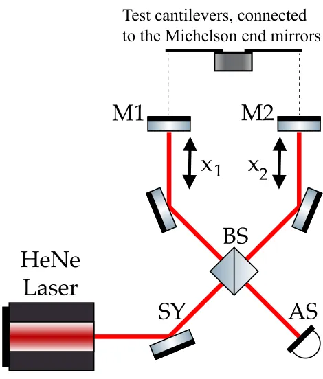
x

₁

x

₂

AS

SY

M1

M2

HeNe

Laser

BS

Test cantilevers, connected to the Michelson end mirrors

Figure 2.2: Simplified schematic of the Michelson Interferometer layout employed. x1 andx2represent the motion of mirrors 1 and 2, which are suspended from test cantilevers 1 and 2 (not shown). “SY” and “AS” refer to the “symmetric” and “anti-symmetric” ports, respectively.

Furthermore, rather than trying to measure the up-conversion events due to ambient seismic motion, we can apply a controlled driving force, equal for both test cantilevers (common mode) to excite more up-conversion events. As will be explained in more detail in Section2.2.3, this also allows us to enhance the apparatus’ sensitivity by incorporating our knowledge of the drive, and can provide insight into the micro-mechanical nature of the up-conversion events.

2.2.1

Utility of the Michelson Interferometer

(31)

We will consider the laser light’s field amplitude incident on the beam splitter to be of the form

Ein = E0eiωt (2.1)

whereωdenotes the frequency of the laser light source, related to the wavelengthλ= 2πc_ω and to the wave numberk = 2π_λ . Then, the field exiting the beam splitter at the AS port will be the superposition of the fields which independently traversed the two arms of the interferometer:

EAS = E1−E2, where (2.2)

Ei = ₂1Eine2ik(L+xi), (2.3)

whereLis the distance from the beam splitter to the equilibrium point of each end mirror and, in the second equation, i= 1,2 refer to the field propagating in the two interferom-eter arms. The minus sign in equation2.2is due to the fact that the field returning from mirror 2 reflects off of the back surface of the beam splitter, and thus experiences aπphase shift relative to the light which reflected off of mirror 1 and the front surface of the beam splitter.

Thus, the field amplitude and intensity at the AS port are given by

EAS = 1₂Eineik2L(eik x1−eik x2) (2.4) IAS= EAS∗ EAS = 1₂Ein2 [1−cos(k(x1−x2))] (2.5)

Equation2.5shows the optical power measured by a photodiode at the AS port, which is a function of the positions of the two end mirrors. Thus, the Michelson interferometer naturally provides an optical signal that is only sensitive to differential displacements of the two test cantilevers, providing, ideally, an infinite rejection of common mode motion.

However, the linear range of the signal is limited by the wavelength of the light used, as can be seen by the sinusoidal functions of the displacement. So, to ensure linear read-out, active feedback is used to keep the interferometer at the proper operating point [38]. Specifically, we employ a feedback loop that stabilizes the differential displacement by applying differential force to the tip of the test cantilevers that is continuously tuned to maintain constant power incident on the photodiode. This does not reduce the infor-mation present in the system, as one can reconstruct the linear open-loop behavior of the system by appropriately combining the feedback control and error signals.

(32)

in equation2.5is linearly proportional to the input laser power. The solution to this is-sue is to read out both interferometer outputs: the symmetric port, as described above, in addition to the anti-symmetric port, “SY”. By injecting the input beam at an angle, one can cleanly separate both output beams.

The signal at the symmetric port can be easily written down by conservation of energy from equation2.5:

ISY = ₂1Ein2 (1+cos(k(x1−x2))) (2.6)

We can now construct a signal that suppresses the linear coupling of intensity to position readout by subtracting the two signals, either with analog electronics or within a digital control and data acquisition system:

xe = ISY− IAS

= E2

incos(k(x1− x2)) (2.7)

With the aid of the feedback control loop, we actuate on the differential mirror positions, which constrains this signal to remain close to zero, which in turn eliminates the direct linear coupling of laser intensity noise to our displacement signal. This interference con-dition is often called thehalf fringe, meaning that the power at the two detectors is equal: half of the input power.

An ideal Michelson interferometer is insensitive to laser frequency noise. However, any mismatch,∆L, in the length of the two Michelson arms will result in a coupling of laser

frequency noise to the output port powers. Indeed, starting from equation2.2and con-sidering that a variation in the laser frequency corresponds to a variation ofk, it is easy to show that a change in the laser frequencyδωwill introduce a power variation equivalent to a differential displacement of the end mirrorδx, given by:

δx= ∆_ωLδω (2.8)

Therefore frequency noise of the laser can be ignored if the length of the two Michelson arms is equalized to within a good accuracy. As discussed below, the safest approach is to implement a way to remotely equalize the length of the two arms.

(33)

motion of the end mirrors, an additional up-conversion mechanism will be present that can mimic the one we are looking for, as discussed below. For this reason it is important to install the two blades in an anti-parallel configuration, and decouple efficiently the mirror angular motion from the cantilever. As discussed below, this is done by suspending the mirrors with thin wires.

2.2.2

Up-conversion Noise Model

Absent a detailed micro-mechanical model, we can instead use a simple phenomenolog-ical model informed by analogous physphenomenolog-ical processes, such as Barkhausen noise in mag-netized materials [39], to design our analysis method. Specifically, we model the effect of up-conversion events in a cantilever spring as a stochastic displacement noise with un-known spectral properties, but with a magnitude determined by the applied force and/or its derivative. Since this stochastic noise is the result of the sum of a large number of mi-croscopic events, its statistical properties depend on the rate and size distribution of such events. We expect those properties to depends both on material properties, and on the local stress or stress rate in each parts of the cantilever. We focus our attention to the case of a cantilever which is subject to a possibly large static load and a time varying external perturbation, typically induced by an external low frequency force. The static load might induce some creep in the metal, but this phenomenon is well known and its magnitude reduces over time [30].

Thus, we consider a cantilever subject to a time dependent forceF(t)_{, with a} character-istic frequency below the macroscopic resonance of the cantilever. In this case, the local microscopic stress varies over time following the external drive. Thus, we write the up-conversion noise contribution to the displacement as:

xup-conversion(t)= χ h

F(t)iδx_f(t)+θhFÛ(t)iδx_j(t) _(2.9)

whereδxfandδxjare stochastic processes representing the force- and jerk-dependent up-conversion, χandθ are the functional forms of the noise dependence on the applied force and its derivative. They reflect the intensity of up-conversion noise in the specific cantilever, and they may be a function of drive frequency and amplitude, in addition to the static load, cantilever geometry and material properties.

(34)

low pass filter with corner frequency of the order of a few Hz. Therefore, whileF(t)_has very low amplitude at higher frequencies, the large amplitudes at low frequency can excite up-conversion events, generating noise in the audio band. Thus, it is important to mea-sure the level of non-linear up-conversions from large static strains and low-frequency motions to noise in the audio band, where Advanced LIGO is most sensitive to gravita-tional waves.

2.2.3

Demodulation Analysis

In order to excite up-conversion events we introduce a low frequency, common mode excitation in the two test cantilevers through the application of a force in the form of F(t)=F₀_sin(ω_dt)_{, that is much larger than the residual seismic motion.}

To mimic the conditions in the Advanced LIGO suspension, this time-varying force is small when compared to the static load applied on the cantilever; in our test setup, for ex-ample, the static load is of the order of 20 N, while the time varying common mode drive is of the order of few mN. Therefore we can expand, by a Taylor series, the two functions

χandθaround the point corresponding to the static load. With this assumption, the individual cantilever displacements are given as:

xi(t)= F0sin_k(ωdt) + √α 2F0sin

(ω_dt)δx_f_,_i(t)+ √β

2F0ωdcos

(ω_dt)δx_j,i(t) _(2.10)

Here,kis the cantilever elastic spring constant and the factors√2 have been introduced to simplify later equations. In the differential displacement signal, the elastic responses of the cantilevers will cancel out, leaving the incoherent sums of the up-conversion noise terms.

(35)

0 2 4 6 8 10 Time [sec]

-4 -3 -2 -1 0 1 2 3 4

[arb.]

Total Signal

Upconverted Noise External Force

Figure 2.3: A qualitative illustration of the signal described in Equation2.11, with sim-ulated data. In this case we have assumed that the up-conversion noise is proportional to the derivative of the external drive, therefore the up-conversion noise power is larger when the sinusoidal excitation crosses zero.

We condense the total differential displacement due to up-conversion noise and some stationary background noisen(t)_{, combining the incoherent sums of up-conversion noise} in each cantilever into a single term:

∆x(t)= n(t)+αF₀_sin(ω_dt)δx_f+βF₀ω_d_cos(ω_dt)δx_j _(2.11)

An example of how theδxjterm manifests itself is shown in Figure2.3.

We now want to take advantage of the periodicity and phase of the envelope of the up-conversion noise processes, and analyze the instantaneous power of the displacement time series, i.e. its square. Simple algebraic computations yield

∆x2(t) = 2n(t)F₀ α_sin(ω_dt)δx_f+ βω_d_cos(ω_dt)δx_j

+n(t)2 + F0 2

h

α2_δ_x2

f + β2ω2dδxj2 i

+ cos(₂ω_dt)F0 2

h

−α2δx2 f +β

2_ω2 dδxj2

i

(36)

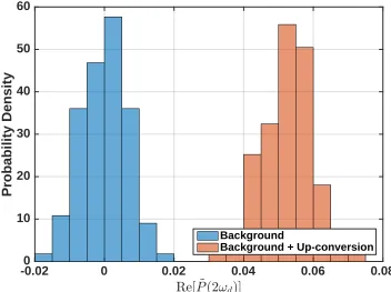
-0.02 0 0.02 0.04 0.06 0.08 Re[ ~P(2!d)]

0 10 20 30 40 50 60

Probability Density

Background

Background + Up-conversion

Figure 2.4: Result of the demodulation described in Equation2.13of 30 minutes of sim-ulated data with background and up-conversion noise levels as in Figure2.3. The distri-butions are clearly separated, showing a strong up-conversion noise signature.

We can average the above quantity over a period longer than the typical time scale of the random processes, and slower than the external drive sinusoid. Assuming thatn(t)_,

δx_f(t)_{, and}δx_j(t)_{are independent zero-mean random noise processes, the first and last} line will have expectation values of zero, while the second line will have some constant expectation value. In contrast, the cos(₂ω_dt)_{term provides a time varying component} at a known frequency, with a known phase with respect to the driving force. Writing the Fourier transform of the power signal asP˜(ω)_{, we can take the expectation value at} 2ωd, ordemodulatethe drive-modulated signal, to see the power fluctuations due to up-conversion events:

< _P˜(₂ω_d)>= F0 4

−α2δx_f2+β2ω2_dδx_j2

(2.13)

In addition, by integrating for many cycles, the determination of the up-conversion noise amplitude of equation 2.13improves proportionally to the square root of integration time. Thus, it is possible to increase the measurement time to find up-conversion noise power varying with the modeled phase and frequency, even below the background noise.

(37)

demodula-tion result of zero, on average. Thus, we can sample the magnitude of the demodulademodula-tion amplitude in two different states: with the drive on and up-conversion noise present, and with the drive off and no up-conversion noise present. We expect to observe different means in the underlying distributions, as shown in Figure2.4.

Thus, the analysis of confidence and uncertainty in our measured results reduces to the standard analysis of whether the two sets of data are unlikely to arise from the same un-derlying probability distribution. Then, appropriate statistical methods, such as the Stu-dent’s t-test, can be used to determine if a statistically significant difference in the means of the two sets of results is present or to derive confidence intervals on the upper bound of the difference in the means consistent with our observations. This manner of statistical validation would provide a strong argument for the observation of up-conversion noise.

In practice, the functional dependence of the up-conversion noise on the applied force is unlikely to take the simple linear form we used above. The model can be generalized by writing out more terms in the Taylor expansion of the χandθfunctions, and working out the corresponding periodic fluctuations expected in the displacement power time series. Thus, by examining different harmonics of the drive frequency, we can poten-tially infer the form ofχand/orθand the micro-mechanical phenomena they arise from. Without going into the details of those computations, it suffices to say that the analysis will be carried out looking at various frequency components of the up-conversion noise amplitude: at the drive frequency, the second and the fourth harmonics. Additionally, we will allow for modulation both in-phase and in quadrature with respect to the drive.

(38)

2.3

The initial prototype of the measurement

system

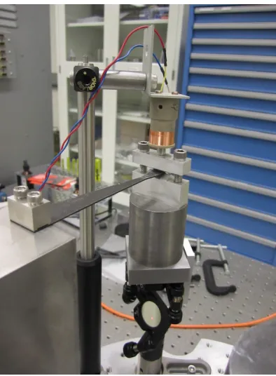
The initial prototype for this experiment consisted of a Michelson interferometer, with end mirrors attached to the bottom of load masses clamped to the tips of small test can-tilevers that were used in Advanced LIGO prototype suspensions. The cancan-tilevers were clamped to a single tall post, and in turn attached to an optical board, where the horizon-tal Michelson interferometer was mounted. The need to measure vertical motion of the test cantilevers while the interferometer was arranged horizontally introduced additional complexity to the system and reduced its overall rigidity.

The load was rigidly clamped to the tip of the test cantilever, as can be seen in Figure2.5. This approach had several drawbacks. First of all, any vertical motion of the cantilever tip coupled directly to a tilt of the load mass and of the Michelson end mirror. In turn, this misalignment of the Michelson was a limiting factor for the maximum amplitude of the common mode displacement we could exert. Secondly, this rigid clamp also cou-pled all of the cantilever transverse and torsional modes to angular motion of the mirror, introducing additional complexity to the actuation and control of the system.

The apparatus was housed in a vacuum chamber to mitigate acoustic noise, and mounted on a stack of two plates standing on rubber springs to reduce seismic noise. Outside of the chamber, a free-running polarized HeNe laser was coupled into a single mode, polarization maintaining, fiber optic cable, which then was fed through to the interior of the chamber.

While the prototype reached a sensitivity on the order of 10−14m /√Hz above 400 Hz, the sensitivity at lower frequencies was greatly limited by poor seismic isolation, as can be seen in Figure2.6. This, in turn, was limited by the available space inside of the available vacuum chamber.

Mitigating these issues became the main consideration when designing the second itera-tion of the experiment. Specifically, we decided to suspend the cantilevers load masses with steel wires to reduce the coupling of higher order vibrational modes of the can-tilevers, and to construct a two stage pendulum seismic isolation system to attempt to reach a sensitivity of 10−15m /√Hz at 10 Hz. This figure is motivated by the sensitivity at which a null result would suggest that up-conversion noise would not be a limiting noise source for Advanced LIGO.

(39)

Figure 2.5: A loaded maraging steel test blade, showing an electromagnetic actuator. One end mirror of the Michelson interferometer is mounted on the bottom of the loading mass.

(40)

101 ₁₀2 ₁₀3

Frequency [Hz] 10−15

10−14

10−13

10−12

10−11

10−10

10−9

10−8

Displacement

ASD

[m/

√

Hz]

Prototype Noise Budget

Shot Noise ADC DAC

Dark Noise Laser Intensity Seismic

Michelson

Figure 2.6: Noise performance of the initial prototype.

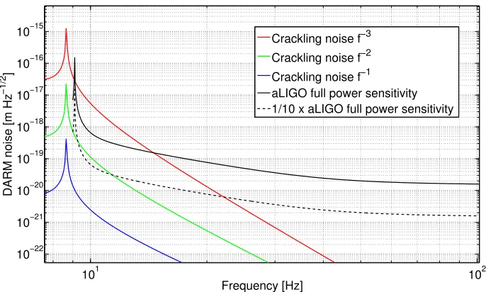
101 102

10−22

10−21

10−20

10−19

10−18

10−17

10−16

10−15

Frequency [Hz]

DARM noise [m Hz

−1/2

]

Crackling noise f−3

aLIGO full power sensitivity 1/10 x aLIGO full power sensitivity

(41)

2.4

The improved measurement system

The limitations found during the operation of the first measurement system prompted us to design an upgraded, more sensitive measurement system. The scientific goal of the improved system is to reach a displacement sensitivity of the differential motion of the tip of the two test cantilevers of the order of 10−15m /√Hz, at frequencies of 10–20 Hz and above, thus improving by many orders of magnitude our capability to detect up-conversion noise in the low frequency region.

This section describes the main features of the improved system: passive suspension of the optical board to achieve better isolation from seismic ground motion; use of a near infrared Nd:YAG source to reduce the laser technical noises; and an improved design of the test cantilever load, clamp and displacement readout.

Figure2.8shows a rendering of the improved instrument. The optical board that holds the Michelson interferometer hangs vertically inside the support structure. The bread-board is suspended by two stages of vertical and horizontal isolation. Its motion is sensed and controlled using six integrated shadow sensor and electromagnetic coil actuators. More details on the seismic isolation system are given in Section2.4.3. The entire sys-tem is housed inside a vacuum chamber, to reduce contamination of the optics, noise due to air fluctuations, and acoustic disturbances.

2.4.1

Optical system

(42)

Support structure

Suspended optical board Cantilever

springs

Displacement sensors

(shadow sensors) and actuators (voice coils)

Suspension wires

Seismic isolation intermediate stage

Figure 2.8: Rendering of the improved measurement apparatus (Section 2.4), show-ing the suspended optical breadboard (Section2.4.1), the seismic isolation system (Sec-tion2.4.3) and the support structure.

cantilevers. Lateral motion of the two blocks is also sensed and mitigated with the same kind of integrated sensors-actuators that are used for the main optical board. Both test cantilevers are clamped to the same support visible in the top center of the board. On the two cantilever tips there are two additional displacement sensors and actuators (not shown in the figure) that are used both to maintain the correct half-fringe operating point of the interferometer and to apply the common mode low frequency drive that would ex-cite up-conversion noise. The symmetric and anti-symmetric beams recombining at the beam splitter are picked up by two additional steering mirrors and sent to two photodi-odes.

(43)

Test maraging cantilevers Suspension

wire _Suspension

wire

Load mass _{Load mass}

Incoming laser beam Input folding and alignment mirror Input folding and alignment mirror

Michelson interferometer

end mirror

folding and alignment mirror Michelson interferometer folding and alignment mirror 50-50

beam splitter

Photodetectors Output port folding mirrors

Suspension wires, to seismic isolation system Optical board, vertically suspended

Figure 2.9: Simplified optical scheme of the Michelson interferometer. Only the main beams and optical components are shown: reflections from the secondary surfaces and beam dumps are not drawn for simplicity. Also, actuators and displacement sensors have been removed.

(44)

be corrected using the translation stage. This procedure allows us to achieve the needed length balancing. The other folding mirror is mounted on a motorized angular stage, to allow us to fine tune the interferometer alignment in vacuum.

2.4.2

Improved test cantilever assembly

The two test cantilevers are pre-curved in such a way that when they are loaded at about 50 % of their yield stress (corresponding to 2.2 kg in our case), they are flat. The transverse profile of the cantilever is triangular: in this way the initial curvature is constant along the entire length of the cantilever, and, moreover, the static stress due to the load is constant along the cantilever, except of course close to the clamp, where there is some localized increase of stress.

The load mass is attached to the cantilever through a single steel wire. In this way we obtain a very high decoupling of any torsional and angular motion of the cantilever tip from angular motions of the Michelson mirror, which is rigidly attached to the bottom of the load mass. Indeed the load mass is isolated from lateral motion of the cantilever tip by a pendulum, and from any angular motion by the stiffness of the wire itself, which can be made very small. Moreover, the wire is clamped to the cantilever with two small steel blocks, held together with bolts. This is a scaled down version of the clamp used in the Advanced LIGO system, and it provides a clean solution that avoids friction and additional stress. Additionally, it serves the purpose of making the test system as similar as possible to the system used in the gravitational wave detectors.

2.4.3

Seismic isolation

(45)

However, there is a limit to the level the two cantilevers can be made equal: in particu-lar, differences in the material, machining, and clamping can result in a mismatch of the resonant frequency and of the distance from the clamp to the wire suspension point. A trade-off is necessary between the requirements on the cantilever equality and the perfor-mance of the seismic isolation system: a worse matching of resonant frequency or distance would require increased performance on the suspension system. It can be shown using a simple elastic model of the two cantilevers that the residual coupling of common vertical motionxcommto differential displacementxdiffof the two cantilever tips is given by:

xdiff xcomm

≈

_f

0 f

2

2δ_ff0 0 +

δL L

(2.14)

Here, f is the measurement frequency, f0is the cantilever mean resonant frequency,δf0 is the difference between the two resonant frequencies,Lis the mean of the cantilever’s length from the clamp to the wire attachment point, andδLis the length mismatch. The two expressions above are correct for frequencies larger than f0(about 2 Hz) and smaller than the first higher order resonance of the loaded cantilever, about 150 Hz.

A difference in the two resonant frequencies of about 5 mHz, obtained experimentally in the first prototype, and a difference in the two lengths of 0.5 mm, well within machin-ing tolerances, provide us with a common mode rejection factor of about 6000. So, to reach the desired displacement sensitivity at 10 Hz, the suspension system must provide an additional factor of 2000 of vertical isolation at 10 Hz. This is achievable using two cas-caded stages with characteristic frequencies close to 2 Hz. Figure2.10shows a simplified schematic of the mechanical system. Each stage is composed of maraging steel cantilevers, roughly 30 cm long, 7 cm wide and 2 mm thick. Four cantilevers suspend the intermedi-ate stage from a support structure with steel wires, and two additional cantilevers support the optical breadboard from the intermediate stage, with another two wires attached to the sides of the board, above its center of mass. Each cantilever supports a load of about 10 kg, which corresponds to about 50 % of their yield stress. Both the optical board and the intermediate stage have a mass of about 20 kg. The intermediate stage includes a stack of rubber to provide some passive damping of the suspension resonant modes.

2.4.4

Current sensitivity and noise sources

(46)

Support upper stage, connected to ground

Cantilever springs for vertical isolation

(x4) _Suspended

intermediate stage Suspension wires (x4)

Rubber

Optical breadboard Cantilever springs for vertical isolation

(x2)

Suspension wire Suspension

wire

First stage of v

er

tical and

hor

iz

on

tal seismic isola

tion

S

ec

ond stage of v

er

tical and

hor

iz

on

tal seismic isola

tion

Figure 2.10: A simplified schematic of the seismic isolation system, highlighting the key components and the two stages of vertical and horizontal isolation.

(47)

101 102 103

Frequency [Hz]

10-16 10-14 10-12 10-10 10-8

Michelson spectrum [m/

Hz]

Seismic Actuation Scattered light Electronic noise Laser intensity noise Shot noise

Current Prototype

Figure 2.11: Typical sensitivity of the measurement system in the present configuration (solid black trace) compared with the best obtained with the first prototype (dotted red line). The other traces show the contribution of various noise sources to the total dis-placement noise: actuation noise and scattered light noises are described in Section2.4.4; electronic noise refers to the sum of photodiode dark noise and analog-to-digital conver-sion noise; laser intensity noise and shot noise are discussed in Section2.2.1.

200 Hz.

(48)

noise is also due to mismatched responses of the suspension cantilevers, this time in their internal resonant modes. This issue will also be mitigated by the addition of the angular decoupling stage as described above.

As discussed in Section2.2, the direct displacement sensitivity is not the ultimate limit to our measurement system, since the demodulation technique can detect periodic non-stationary noise below the sensing noise, provided that the latter is non-stationary. There-fore particular care is necessary for all sources of non-stationary noise, especially those that might be modulated by the common mode motion of the two cantilevers. Referring again to Figure2.11, two of the noise sources listed there are particularly problematic. Scat-tered light is intrinsically non-stationary, since the amplitude and maximum frequency of this noise source depends on the motion of the scattering element [42]. Scattered light has been mitigated with a careful placement of black glass absorbing baffles and beam dumps. All spurious beams from the anti-reflection coated surfaces are intercepted and dumped. This improvement will be sufficient to reduce scattered light below the target sensitivity. In addition the increased seismic isolation will also help reducing scattered light. Indeed, scattered light up-conversion is highly non linear [42]: residual motion at few Hz will be the dominant contributor to scattered light phase noise, while the slower ≈_{100 mHz motion that we will introduce to periodically stress the cantilevers results in a} negligible contribution. The second potentially problematic non-stationary noise source can be traced to the actuation chain used to apply force on the two test cantilevers. In par-ticular, the digital-to-analog converters (DAC) are known to exhibit a significant amount of harmonic distortion. The low frequency common mode drive is up-converted in fre-quency by the DAC and results in a non stationary noise at the level of the measured sensitivity. This issue is being tackled with an improvement of the control electronics.

(49)

2.5

Discussion and outlook

This chapter presented an instrument designed for the study of the mechanical up-con-version phenomenon in metals. Two key points make the approach presented here differ-ent from previous studies. First of all, given the authors’ involvemdiffer-ent in the gravitational wave observatory Advanced LIGO, this system will study the behavior of metals in the elastic regime, far from the yield stress that would introduce plastic deformations. As already pointed out, to the best of our knowledge there has been no experimental inves-tigations of this kind in this