Volume 2009, Article ID 859698,7pages doi:10.1155/2009/859698
Research Article
An Adaptive Nonlinear Filter for System Identification
Ifiok J. Umoh (EURASIP Member) and Tokunbo Ogunfunmi
Department of Electrical Engineering, Santa Clara University, Santa Clara, CA 95053, USA
Correspondence should be addressed to Tokunbo Ogunfunmi,[email protected]
Received 12 March 2009; Accepted 8 May 2009
Recommended by Jonathon Chambers
The primary difficulty in the identification of Hammerstein nonlinear systems (a static memoryless nonlinear system in series with a dynamic linear system) is that the output of the nonlinear system (input to the linear system) is unknown. By employing the theory of affine projection, we propose a gradient-based adaptive Hammerstein algorithm with variable step-size which estimates the Hammerstein nonlinear system parameters. The adaptive Hammerstein nonlinear system parameter estimation algorithm proposed is accomplished without linearizing the systems nonlinearity. To reduce the effects of eigenvalue spread as a result of the Hammerstein system nonlinearity, a new criterion that provides a measure of how close the Hammerstein filter is to optimum performance was used to update the step-size. Experimental results are presented to validate our proposed variable step-size adaptive Hammerstein algorithm given a real life system and a hypothetical case.
Copyright © 2009 I. J. Umoh and T. Ogunfunmi. This is an open access article distributed under the Creative Commons Attribution License, which permits unrestricted use, distribution, and reproduction in any medium, provided the original work is properly cited.
1. Introduction
Nonlinear system identification has been an area of active research for decades. Nonlinear systems research has led to the discovery of numerous types of nonlinear systems such as Volterra, Hammerstein, and Weiner nonlinear systems [1–4]. This work will focus on the Hammerstein nonlinear system depicted in Figure 1. Hammerstein nonlinear models have been applied to modeling distortion in nonlinearly ampli-fied digital communication signals (satellite and microwave links) followed by a linear channel [5, 6]. In the area of biomedical engineering, the Hammerstein model finds application in modeling the involuntary contraction of human muscles [7, 8] and human heart rate regulation during treadmill exercise [9]. Hammerstein systems are also applied in the area of Neural Network since it provides a convenient way to deal with nonlinearity [10]. Existing Hammerstein nonlinear system identification techniques can be divided into three groups:
(i) deterministic techniques such as orthogonal least-squares expansion method [11–13],
(ii) stochastic techniques based on recursive algorithms [14,15] or nonadaptive methods [16], and
(iii) adaptive techniques [17–20].
Polynomial nonlinearity
Hammerstein nonlinear filter
Infinite impulse
response filter
d(n)
x(n) e(n)
v(n)
Plant (unknown system)
d(n)
z(n)
Figure1: Adaptive system identification of a Hammerstein system model.
convergence while maintaining a small misadjustment and computational complexity, the Affine Projection theory is used as opposed to LMS [18] or Recursive Least squares (RLSs).
In nonlinear system identification, input signals with high eigen value spread, ill-conditioned tap input autocorre-lation matrix can lead to divergence or poor performance of a fixed step-size adaptive algorithm. To mitigate this problem, a number of variable step-size update algorithms have been proposed. These variable step-size update algorithms can be roughly divided into gradient adaptive step-size [21, 22] and normalized generalized gradient descent [23]. The major limitation of gradient adaptive step-size algorithms is their sensitivity to the time correlation between input signal samples and the value of the additional step-size parameter that governs the gradient adaptation of the step-size. As a result of these limitations, a criteria for the choice of the step-size based on Lyapunov stability theory is proposed to track the optimal step-size required to maintain a fast convergence rate and low misadjust-ment.
In this paper, we focus on the adaptive system identifi-cation problem of a class of Hammerstein output error type nonlinear systems with polynomial nonlinearity. Our unique contributions in the paper are as follows.
(1) Using the theory of affine projections [24], we derive an adaptive Hammerstein algorithm that identifies the linear subsystem of the Hammerstein system without prior knowledge of the input signalz(n).
(2) Employing the Lyapunov stability theory, we develop criteria for the choice of the algorithms step-size which ensures the minimization of the Lyapunov function. This is particularly important for the stability of the linear algorithm regardless of the location of the poles of the IIR filter.
Briefly, the paper is organized as follows. Section 2 describes the nonlinear Hammerstein system
identifica-tion problem addressed in this paper. Section 3 contains a detailed derivation of the proposed variable step-size adaptive Hammerstein algorithm. Section 4 provides both a hypothetical and real life data simulation validating the effectiveness of the variable step-size adaptive algorithm proposed. Finally, we conclude with a brief summary in Section 5.
2. Problem Statement
Consider the Hammerstein model shown inFigure 1, where
x(n),v(n), andd(n) are the systems input, noise, and output, respectively. z(n) represents the unavailable internal signal output of the memoryless polynomial nonlinear system. The output of the memoryless polynomial nonlinear system, which is the input to the linear system, is given by
z(n)=
L
l=1
pl(n)xl(n). (1)
Let the discrete linear time-invariant system be an infinite impulse response (IIR) filter satisfying a linear difference equation of the form
d(n)= −
N
i=1
ai(n)d(n−i) + M
j=0 bj(n)z
n−j, (2)
where pl(n), ai(n), and bj(n) represent the coefficients of
the nonlinear Hammerstein system at any given timen. To ensure uniqueness, we setb0(n) = 1 (any other coefficient other thanb0(n) can be set to 1). Thus, (2) can be written as
d(n)=
L
l=1
pl(n)xl(n)− N
i=1
ai(n)d(n−i) + M
j=1 bj(n)z
n−j.
Let
θ(n)=[a1(n) · · · aN(n)b1(n) · · · bM(n)
p1(n) · · · pL(n)
H
,
b0=1,
s(n)=−d(n−1) · · · −d(n−N)
z(n−1) · · · z(n−M)
x(n) · · · xL(n) H.
(4)
Equation (3) can be rewritten in compact form
d(n)=s(n)Hθ(n). (5)
The goal of the Adaptive nonlinear Hammerstein system identification is to estimate the coefficient vector (θ(n)) in (5) of the nonlinear Hammerstein filter based only on the input signalx(n) and output signald(n) such that d(n) is close to the desired response signald(n).
3. Adaptive Hammerstein Algorithm
In this section, we develop an algorithm based on the theory of Affine projection [24] for estimation of the coefficients of the nonlinear Hammerstein system using the plant input and output signals. The main idea of our approach to nonlinear Hammerstein system identification is to formulate a criterion for designing a variable step-size affine projection Hammerstein filter algorithm and then use the criterion in minimizing the cost function.
3.1. Stochastic Gradient Minimization Approach. We formu-late the criterion for designing the adaptive Hammerstein filter as the minimization of the square Euclidean norm of the change in the weight vector
θ(n)=θ(n)−θ(n−1) (6)
subject to the set ofQconstraints
dn−q=sn−qHθ(n) q=1,. . .,Q. (7)
Applying the method of Lagrange multipliers with multiple constraints to (6) and (7), the cost function for the affine projection filter is written as (assuming real data)
J(n−1)=θ(n)−θ(n−1)2+ Re[(n−1)λ], (8)
where
(n−1)=d(n−1)−S(n−1)Hθ(n),
d(n−1)=[d(n−1) · · · d(n−Q)]H,
S(n−1)=[s(n−1) · · · s(n−Q)],
λ=λ1 · · · λQ
H .
(9)
Minimizing the cost function (8) (squared prediction error) with respect to the nonlinear Hammerstein filter weight vectorθ(n) gives
∂J(n−1)
∂θ(n) =2
θ(n)−θ(n−1)−∂
θ(n)HS(n−1)λ
∂θ(n) , (10)
where
∂θ(n)HS(n−1)
∂θ(n)
=
∂θ(n)Hs(n−1)
∂θ(n) · · ·
∂θ(n)Hs(n−Q)
∂θ(n)
.
(11)
Since a portion of the vectorss(n) inS(n) include past
d(n) which are dependent on pastθ(n) which are used to form the newθ(n), the partial derivative of each element in (10) gives
∂θ(n)Hsn−q ∂ai(n) = −
dn−q−i−
N
k=1 ak(n)∂
dn−q−k ∂ai(n)
,
(12)
∂θ(n)Hsn−q ∂bj(n) =z
n−q−j−
N
k=1 ak(n)∂
dn−q−k ∂bj(n) ,
(13)
∂θ(n)Hsn−q ∂pl(n) =x
ln−q+ M
k=1 bk(n)
∂zn−q−k ∂pl(n)
−
N
k=1 ak(n)∂
dn−q−k ∂pl(n) .
(14)
From (12), (13), and (14) it is necessary to evaluate the derivative of past d(n) with respect to current weight estimates. In evaluating the derivative ofd(n) with respect to the current weight vector, we assume that the step-size of the adaptive algorithm is chosen such that [24]
θ(n)∼=θ(n−1)∼= · · · ∼=θ(n−N). (15)
Therefore
ai(n)∼=ai(n−1)∼= · · · ∼=ai(n−N),
∂dn−q ∂ai(n) = −
dn−q−i−
N
k=1 ak(n)∂
dn−q−k ∂ai(n−k)
bj(n)∼=bj(n−1)∼= · · · ∼=bj(n−N),
,
∂dn−q ∂bj(n) =z
n−q−j−
N
k=1 ak(n)∂
dn−q−k ∂bj(n−k)
,
pl(n)∼=pl(n−1)∼= · · · ∼=pl(n−N),
(17)
∂dn−q ∂pl(n) =x
ln−q+ M
k=1 bk(n)∂z
n−q−k ∂pl(n−k) .
−
N
k=1 ak(n)∂
dn−q−k ∂pl(n−k)
,
(18)
∂pl
n−q−k ∂pl(n−k) =
1, (19)
thus,
∂dn−q ∂pl(n) =x
ln−q+ M
k=1 bk(n)xl
n−q−k
−
N
k=1 ak(n)∂
dn−q−k ∂pl(n−k) ,
(20)
where
φn−q= ∂d
n−q ∂θ(n)
= ⎡
⎣∂dn−q
∂a1(n) · · ·
∂dn−q ∂aN(n)
∂dn−q ∂b1(n)
· · · ∂d
n−q ∂bM(n)
∂dn−q ∂p1(n) · · ·
∂dn−q ∂pL(n)
⎤ ⎦
H
.
(21)
Let
Φ(n−1)=∂
θ(n)HS(n−1)
∂θ(n) ,
ψn−q=
−dn−q−1 · · · −dn−q−Nzn−q−1
· · · zn−q−M M
j=0
xn−q−j
· · ·
M
j=0
xLn−q−j
⎤ ⎦
H
,
Ψ(n−1)=ψ(n−1) · · · ψ(n−Q).
(22)
Substituting (16), (17), and (20) into (11), we get
Φ(n−1)=Ψ(n−1)−
N
k=1
ak(n−1)Φ(n−1−k). (23)
Thus, rewriting (10)
∂J(n−1)
∂θ(n) =2
θ(n)−θ(n−1)−Φ(n−1)λ. (24)
Setting the partial derivative of the cost function in (24) to zero, we get
θ(n)= 1
2Φ(n−1)λ. (25)
From (7), we can write
d(n−1)=S(n−1)Hθ(n), (26) where
d(n−1)=[d(n−1) · · · d(n−Q)],
d(n−1)=S(n−1)Hθ(n−1) +1
2S(n−1)
HΦ(n−
1)λ.
(27)
Evaluating (27) forλresults in
λ=2S(n−1)HΦ(n−1)−1e(n−1), (28) where
e(n−1)=d(n−1)−S(n−1)Hθ(n−1). (29) Substituting (28) into (25) yields the optimum change in the weight vector
θ(n)=Φ(n−1)S(n−1)HΦ(n−1)−1e(n−1). (30) Assuming that the input to the linear part of the nonlinear Hammerstein filter is a memoryless polynomial nonlinearity, we normalize (30) as in [25] and exercise con-trol over the change in the weight vector from one iteration to the next keeping the same direction by introducing the step-sizeμ. Regularization of theS(n−1)HΦ(n−1) matrix is also used to guard against numerical difficulties during inversion, thus yielding
θ(n)=θ(n−1)−μΦ(n−1)
×ΦδI+μS(n−1)H(n−1)−1e(n−1).
(31)
To improve the update process Newton’s method is applied by scaling the update vector byR−1(n). The matrixR(n) is
recursively computed as
R(n)=λnR(n−1) + (1−λn)Φ(n−1)Φ(n−1)H, (32)
whereλnis typically chosen between 0.95 and 0.99. Applying
the matrix inversion lemma on (32) and using the result in (31), the new update equation is given by
θ(n)=θ(n−1)−μR(n−1)−1Φ(n−1)
3.2. Variable Step-Size. In this subsection, we derive an update for the step-size using a Lyapunov function of summed squared nonlinear Hammerstein filter weight esti-mate error. The variable step-size derived guarantees the stable operation of the linear IIR filter by satisfying the stability condition for the choice ofμin [26]. Let
θ(n)=θ−θ(n), (34)
where θ represents the optimum Hammerstein system coefficient vector. We propose the Lyapunov functionV(n) as
V(n)=θ(n)Hθ(n), (35)
which is the general form of the quadratic Lyapunov function [27]. The Lyapunov function is positive definite in a range of values close to the optimum θ = θ(n). In order for the multidimensional error surface to be concave, the time derivative of the Lyapunov function must be semidefinite. This implies that
ΔV(n)=V(n)−V(n−1)≤0. (36)
From the Hammerstein filter update equation
θ(n)=θ(n−1)−μΦ(n−1)S(n−1)HΦ(n−1)−1e(n−1), (37)
we subtractθfrom both sides to yeild
θ(n)=θ(n−1)−μΦ(n−1)S(n−1)HΦ(n−1)−1e(n−1).
(38)
From (35), (36), and (38) we have
ΔV(n)=θ(n)Hθ(n)−θ(n−1)Hθ(n−1). (39)
Minimizing the Lyapunov function with respect to the step-size μ, and equating the result to zero, we obtain the optimum value forμasμopt
μopt=E
θ(n−1)HΦ(n−1)S(n−1)HΦ(n−1)−1e(n−1)
Ee(n−1)HΥ(n−1)HΥ(n−1)e(n−1) , (40)
where
Υ(n−1)=Φ(n−1)S(n−1)HΦ(n−1)−1. (41)
Adding the system noisev(n) to the desired output and assuming that the noise is independently and identically distributed and statistically independent ofS(n), we have
d(n)=S(n)Hθ+v(n). (42)
INITIALIZE:R−1(0)=I,λ
n=/0, 0< β≤1 forn=0 to sample size do
e(n−1)=d(n−1)−S(n−1)Hθ(n−1)
Φ(n−1)=Ψ(n−1)−N k=1
ak(n−1)Φ(n−1−k)
B(n)=αB(n−1)−(1−α)Υ(n−1)e(n−1)
μ(n)=μopt(
B(n)2 B(n)2+C)
( λn 1−λn
I−Φ(n−1)HR(n−1)−1Φ(n−1))
−1
R(n)−1=λ1
n[R(n−1)
−1−R(n−1)−1Φ(n−1)
Φ(n−1)HR(n−1)−1]
θ(n)=θ(n−1)−μ(n)R(n)−1Φ(n−1) (δI+μ(n)S(n−1)HΦ(n−1))−1e(n−1)
z(n)=x(n)Hp(n)
d(n)=s(n)Hθ(n) end for
Algorithm1: Summary of the proposed Variable Step-size
Ham-merstein adaptive algorithm.
From (40) we write
μoptEe(n−1)HΥ(n−1)HΥ(n−1)e(n−1)
=E
θ(n−1)HΦ(n−1)S(n−1)HΦ(n−1)−1e(n−1)
.
(43)
The computation ofμoptrequires the knowledge ofθ(n−1) which is not available during adaptation. Thus, we propose the following suboptimal estimate forμ(n):
μ(n)= μoptE Υ(n−1)e(n−1)
2
EΥ(n−1)e(n−1)2+σ2 vTr
EΥ(n−1)2.
(44)
We estimateEΥ(n−1)e(n−1)by time averaging as follows:
B(n)=αB(n−1)−(1−α)Υ(n−1)e(n−1)
μ(n)=μopt ⎛ ⎜ ⎝
B(n)2
B(n)2
+C
⎞ ⎟
⎠, (45)
where μopt is an rough estimate of μopt, α is a smoothing factor (0 < α < 1), and C is a constant representing
σ2
vTr{Υ(n−1)2} ≈Q/SNR. We guarantee the stability of
the Hammerstein filter by choosingμopt to satisfy the stability bound in [26]. Choosingμopt to satisfy the stability bound [26] will bound the step-size updateμ(n) with an upper limit ofμopt thereby ensuring the slow variation and stability of the linear IIR filter.
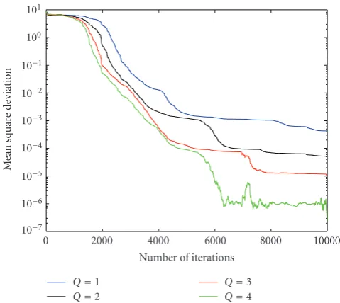
Q=1
Q=2
Q=3
Q=4
0 2000 4000 6000 8000 10000
Number of iterations 10−7
10−6 10−5 10−4 10−3 10−2 10−1 100 101
M
ean
squar
e
de
vi
ation
Figure2: Mean square deviation learning curve of the proposed
algorithm for varying constraint.
of feedback, M the number of feedforward coefficients for the linear subsystem, and L the number of coef-ficients for the polynomial subsystem. Based on these coefficient numbers, let K represent N + M + L − 2 in the computation of the computational cost of our proposed adaptive nonlinear algorithm. In computing the computational cost, we assume that the cost of invert-ing a K × K matrix is (K3) (Multiplications and
additions) and (L2N) for computing R−1 [28]. Under
these assumptions, the computational cost of our pro-posed algorithm is of (QK2) multiplications compared
to (K2) in [17]. This increase in complexity due to
the order of the input regression matrix in the proposed algorithm is compensated for by the algorithms good performance.
4. Simulation Results
In this section, we validate the proposed algorithm with simulation results corresponding to two different types of input signals (white and highly colored signals). The white signal was an additive white Gaussian noise signal of zero mean and unity variance. The highly colored signal was generated by filtering the white signal with a filter of impulse response:
H1(z)= 0.5
1 + 0.9z−1. (46)
The Hammerstein system was modeled such that the dynamic linear system had an impulse response H2(z) given by
Q=1
Q=2
Q=3
Q=4 Ref. [17]
0 2000 4000 6000 8000 10000
Number of iterations 10−6
10−5 10−4 10−3 10−2 10−1 100 101 102
M
ean
squar
e
de
vi
ation
Figure3: Mean square deviation learning curves of the proposed
algorithm for varying constraint and a colored input signal.
H2(z)
=1.0000−1.8000z−1+1.6200z−2−1.4580z−3+0.6561z−4 1.0000−0.2314z−1+0.4318z−2−0.3404z−3+0.5184z−4,
(47)
and static nonlinearity modeled as a polynomial with coefficients
z(n)=x(n)−0.3x(n)2+ 0.2x(n)3. (48)
The desired response signald(n) of the adaptive Ham-merstein filter was obtained by corrupting the output of the unknown system with additive white noise of zero mean and variance such that the output signal to noise ratio was 30 dB. The proposed algorithm was initialized as follows:
λn=0.997,μopt=1.5e−6,δ=5e−4, andC=0.0001. Figure 2shows the mean square deviation between the estimated and optimum Hammerstein filter weights for a white input case. The results were obtained, by ensemble averaging over 100 independent trials. The figure shows that the convergence speed of the proposed algorithm is directly correlated to the number of constraintsQused in the algorithm.
5. Conclusion
We have proposed a new adaptive filtering algorithm for the Hammerstein model filter based on the theory of Affine Projections. The new algorithm minimizes the norm of the projected weight error vector as a criterion to track the adaptive Hammerstein algorithm’s optimum performance. Simulation results confirm the convergence of the parameter estimates from our proposed algorithm to its corresponding parameter in the plants parameter vector.
References
[1] T. Ogunfunmi, Adaptive Nonlinear System Identification: Volterra and Wiener Model Approaches, Springer, London, UK, 2007.
[2] V. J. Mathews and G. L. Sicuranza,Polynomial Signal Process-ing, John Wiley & Sons, New York, NY, USA, 2000.
[3] T. Ogunfunmi and S. L. Chang, “Second-order adaptive Volterra system identification based on discrete nonlinear Wiener model,” IEE Proceedings: Vision, Image and Signal Processing, vol. 148, no. 1, pp. 21–30, 2001.
[4] S.-L. Chang and T. Ogunfunmi, “Stochastic gradient based third-order Volterra system identification by using nonlinear Wiener adaptive algorithm,” IEE Proceedings: Vision, Image and Signal Processing, vol. 150, no. 2, pp. 90–98, 2003. [5] W. Greblicki, “Nonlinearity estimation in Hammerstein
sys-tems based on ordered observations,”IEEE Transactions on Signal Processing, vol. 44, no. 5, pp. 1224–1233, 1996. [6] S. Prakriya and D. Hatzinakos, “Blind identification of linear
subsystems of LTI-ZMNL-LTI models with cyclostationary inputs,”IEEE Transactions on Signal Processing, vol. 45, no. 8, pp. 2023–2036, 1997.
[7] K. J. Hunt, M. Munih, N. N. de Donaldson, and F. M. D. Barr, “Investigation of the hammerstein hypothesis in the modeling of electrically stimulated muscle,”IEEE Transactions on Biomedical Engineering, vol. 45, no. 8, pp. 998–1009, 1998. [8] D. T. Westwick and R. E. Kearney,Identification of Nonlinear
Physiological Systems, John Wiley & Sons, New York, NY, USA, 2003.
[9] S. W. Su, L. Wang, B. G. Celler, A. V. Savkin, and Y. Guo, “Identification and control for heart rate regulation during treadmill exercise,”IEEE Transactions on Biomedical Engineering, vol. 54, no. 7, pp. 1238–1246, 2007.
[10] D. P. Mandic and J. A. Chambers,Recurrent Neural Networks for Prediction: Learning Algorithms, Architectures and Stability, John Wiley & Sons, Chichester, UK, 2001.
[11] F. Ding, Y. Shi, and T. Chen, “Auxiliary model-based least-squares identification methods for Hammerstein output-error systems,”Systems and Control Letters, vol. 56, no. 5, pp. 373– 380, 2007.
[12] E.-W. Bai, “Identification of linear systems with hard input nonlinearities of known structure,”Automatica, vol. 38, no. 5, pp. 853–860, 2002.
[13] F. Giri, F. Z. Chaoui, and Y. Rochdi, “Parameter identification of a class of Hammerstein plants,”Automatica, vol. 37, no. 5, pp. 749–756, 2001.
[14] M. Boutayeb, H. Rafaralahy, and M. Darouach, “A robust and recursive indentificaition method for Hammerstein model,” inProceedings of the IFAC World Congress, pp. 447–452, San Francisco, Calif, USA, 1996.
[15] J. V¨or¨os, “Iterative algorithm for parameter identification of Hammerstein systems with two-segment nonlinearities,”IEEE Transactions on Automatic Control, vol. 44, no. 11, pp. 2145– 2149, 1999.
[16] E.-W. Bai, “An optimal two-stage identification algorithm for Hammerstein-Wiener nonlinear systems,”Automatica, vol. 34, no. 3, pp. 333–338, 1998.
[17] J. Jeraj and V. J. Mathews, “A stable adaptive Hammerstein fil-ter employing partial orthogonalization of the input signals,”
IEEE Transactions on Signal Processing, vol. 54, no. 4, pp. 1412– 1420, 2006.
[18] E.-W. Bai, “A blind approach to the Hammerstein-Wiener model identification,”Automatica, vol. 38, no. 6, pp. 967–979, 2002.
[19] I. J. Umoh and T. Ogunfunmi, “An adaptive algorithm for Hammerstein filter system identification,” inProceedings of the 16th European Signal Processing Conference (EUSIPCO ’08), Lausanne, Switzerland, August 2008.
[20] F. Ding, T. Chen, and Z. Iwai, “Adaptive digital control of Hammerstein nonlinear systems with limited output sam-pling,”SIAM Journal on Control and Optimization, vol. 45, no. 6, pp. 2257–2276, 2007.
[21] V. J. Mathews and Z. Xie, “Stochastic gradient adaptive filter with gradient adaptive step size,”IEEE Transactions on Signal Processing, vol. 41, no. 6, pp. 2075–2087, 1993.
[22] A. Benveniste, M. Metivier, and P. Priouret,Adaptive Algo-rithms and Stochastic Approximation, Springer, New York, NY, USA, 1990.
[23] D. P. Mandic, “A generalized normalized gradient descent algorithm,”IEEE Signal Processing Letters, vol. 11, no. 2, part 1, pp. 115–118, 2004.
[24] S. Haykin,Adaptive Filter Theory, Prentice-Hall, Upper Saddle River, NJ, USA, 4th edition, 2002.
[25] N. J. Bershad, “On the optimum data nonlinearity in LMS adaptation,”IEEE Transactions on Acoustics, Speech, and Signal Processing, vol. 34, no. 1, pp. 69–76, 1986.
[26] A. Carini, V. John Mathews, and G. L. Sicuranza, “Sufficient stability bounds for slowly varying direct-form recursive linear filters and their applications in adaptive IIR filters,” IEEE Transactions on Signal Processing, vol. 47, no. 9, pp. 2561–2567, 1999.
[27] C. R. Johnson Jr., “Adaptive IIR filtering: current results and open issues,”IEEE Transactions on Information Theory, vol. 30, no. 2, pp. 237–250, 1984.