Article
Flexibility of Boolean Network Reservoir Computers in Approximating
Arbitrary Recursive and Non-recursive Binary Filters
Moriah Echlin1,2, Boris Aguilar1, Max Notarangelo1, David L Gibbs1, Ilya Shmulevich1,*
1 Institute for Systems Biology; 401 Terry Ave N, Seattle, WA 98109, USA
2 Molecular & Cellular Biology Program, University of Washington; Seattle, WA 98195, USA * Correspondence: [email protected]
Keywords: complex adaptive systems; systems dynamics; dynamical systems; signal processing; reservoir computing; machine learning; Boolean networks; biological modeling
Abstract
Reservoir computers (RCs) are a biology inspired computational framework for signal processing typically implemented using recurrent neural networks. Recent work has shown that Boolean networks (BN) can also be used as reservoirs. We analyze the performance of BN RCs, measuring their flexibility and identifying factors that determine effective approximation of Boolean functions that are applied in a sliding-window fashion over a binary signal, either non-recursively or non-recursively. We train and test BN RCs of different sizes, signal connectivity, and in-degree to approximate 3-bit, 5-bit and 3-bit recursive binary functions. We analyze how BN RC parameters and function average sensitivity, a measure of function smoothness, affect approximation accuracy as well as the spread of accuracies for a single reservoir. We found that approximation accuracy and reservoir flexibility are highly dependent on RC parameters.
Overall, our results indicate that not all reservoirs are equally flexible and RC instantiation and training can be more efficient if this is taken into account. The optimum range of RC parameters opens up an angle of exploration for understanding how biological systems might be tuned to balance system restraints with processing capacity.
Introduction
Fruit flies use their olfactory system to differentiate between odors and in doing so, they map similar odors to similar neural responses. The odor molecules are essentially an input data stream. To process this input, the molecules are captured by odorant receptor neurons that feed a set of 50 projection neurons. The projection neurons, operating in 50-dimensional space, are expanded further into a higher dimension of 2000, stored by so-called Kenyon cells, and followed by the classification (locality sensitive hashing) that takes place in that high dimension [1].
Many biological systems are regarded as non-linear dynamical systems [2] operating in high-dimensional space. For example, proteins, genes, and macromolecules interact in a variety of ways to create the dynamics of cells [3]. Collections of cells interact and coordinate activity, forming cohesive units such as bacterial colonies, simple multicellular organisms, or tissues in more complex multicellular organisms. At each level of organization, ‘input’ signals (e.g., odors or hormones) are introduced into the system, processed by means of the system’s dynamics,
and responded to accordingly, sometimes generating new ‘output’ signals as a byproduct [4]. Fundamentally, biological systems must process external signals in real time to inform a wide variety of response decisions.
In this vein, reservoir computing (RC) is a form of signal processing used for
classification and online learning that uses such high-dimensional systems to process signals. Initially called echo state networks [2] or liquid state machines [5], the computational structure resembles an unorganized recurrent neural network. These networks were inspired by the most classical example of signal processing in biological systems — the brain. While initial research in neural networks was focused on modeling and understanding neural computation [6]
applications and directions for research quickly expanded in scope. For reservoir computers, this includes systems for predicting time series from chaotic systems [7,8] as well as multiple real-world applications such as gas detection [9], robotics [10–12], and economic trends [13], Applications in processing human data are also found with human emotion [14] and gesture recognition [15], speech and text processing [16,17], and health care monitoring [18].
In biology, reservoir computers have been used to analyze biological data for identifying anomalous states such as cardiac arrhythmia [19], seizures [20,21], and microsleeps [22] as well as for high-dimensional classification such as cell type detection [23]. In these applications, RCs are used to interpret or classify biological data. RCs have also been used as models of biological systems, serving to explore the mechanisms and dynamics of said systems. For example, the questions of how the brain functions [24-26] and how gene regulatory networks respond to external stimuli [27,28] have been studied in an RC context.
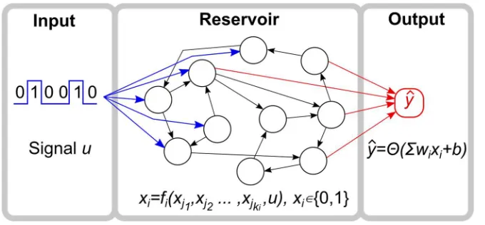
In reservoir computing, an incoming signal is fed into the reservoir, a randomly connected recurrent network where nodes are connected via a variety of coupling functions. Thus, the reservoir transforms the signal into a high-dimensional representation. Finally, an output layer is trained, often with straightforward techniques such as regularized regression [29], to perform a classification or regression task (Fig. 1).
RCs can also be trained to act as signal processors, filtering the input to produce a new output. This can be through approximating a function that is normally applied to a window sliding over the signal. The type of function can be extended to recursive functions, where some
elements of the input-window are replaced by values from previously generated outputs. These types of filters have a long history of use which includes filtering biological signals [30–32].
Implementation of Boolean networks, both in software and in hardware, is also considerably easier and faster than more traditional approaches [41].
Similar to neural networks, Boolean networks were first used as models of biological systems, namely gene regulatory networks [37,42,43]. While often researched to understand cellular behavior in terms of protein/gene interaction networks in isolation [44–46], BNs have also been used to understand how external signals impact biological systems [47–49]. These systems rely on their ability to process external signals (relevant to survival or population function) and make decisions based on them in real time, thereby performing a similar computation that a reservoir does [4]. Just as the Boolean network framework has provided insight into how biological systems function, studying BN reservoir computers (BN RCs) may further our understanding of biological signal-response.
Previous work on BNs as reservoirs is still limited. Snyder et al. [38,50] evaluated BN RCs with different numbers of nodes (𝑁) and average node input degrees (𝐾). Using a measure of reservoir quality, it was found that, compared to networks with homogeneous in-degree, networks with heterogeneous in-degree better separated inputs by class, the so-called separability property [5]. Also, it was found that computational ability - when the difference in separability and fading memory is greatest - was maximized when the average in-degree was𝐾 = 2 (out of 𝐾=1,2,3) [50]., and that higher 𝐾led to worse performance. This value for 𝐾 is notable, as Boolean networks with 𝐾= 2 are known to be dynamically critical (Lyapunov exponent = 0). Critical dynamics, which lie at the border between order and chaos, have been shown to be important in computation and information processing, biological and otherwise [51-55].
While previous work [38,50] has laid the foundation showing that it is possible to use Boolean networks as reservoirs, the main focus has been on testing a small number of well-known functions, such as the median and parity functions, as benchmark measures. We are extending the body of research in three ways: (1) by performing a wider examination of how well these systems perform across different functions, including recursively defined operators, (2) by analyzing how flexible a single reservoir is for repurposing (i.e., retraining only the output layer and keeping the same network reservoir), and (3) characterizing the functions that are easier or harder for the reservoir to implement in terms of the function’s average sensitivity, which is a measure of its smoothness. We also evaluate reservoirs under different dynamical regimes: ordered, critical, chaotic.
Materials and Methods
Reservoir Computer
function, which captures the error between the reservoir output and the function to be approximated.
Reservoir
In our implementation, the reservoir is constructed as a random Boolean network (RBN) [37]. RBNs are networks with 𝑁binary-valued nodes with states
𝑋 = {𝑥 , 𝑥 , . . . , 𝑥 } 𝑥 ∈ {0,1}, 𝑖 = 1, . . . , 𝑁, 𝑡 > 0.
The state of the network at any time, 𝑋 , is a function of the state at the previous time, 𝑋 , given by
𝑋 = 𝐹(𝑋 )
where
𝐹 = { 𝑓 , 𝑓 , . . . , 𝑓 }
is the set of Boolean updating functions corresponding to each node. The node in-degree need not be constant, such that each function 𝑓has an independent number of arguments, 𝑘, so that
𝑥 = 𝑓 (𝑥 , 𝑥 , . . . , 𝑥 ).
The identity of each of the 𝑘 arguments is chosen randomly from the 𝑁 nodes, without replacement. The in-degree of the whole network is characterized by the average in-degree across its nodes, 𝐾. The other primary descriptor of the network is the bias, 𝑝, which is the probability that a function outputs a 1. Together, 𝑝 and 𝐾 can be varied to adjust the dynamics of the network - from ordered, in which perturbations die out, to chaotic, in which perturbations are amplified [39,40]. For this paper, we will fix 𝑝= 0.5 and tune the dynamics of the networks by varying 𝐾. Generally we tune the dynamics using 𝐾< 2 for ordered, 𝐾= 2 for near critical, 𝐾> 2 for chaotic. To construct a network with a specific 𝐾, we take 𝐾 ⋅ 𝑁 edges uniformly distributed amongst all pairs of nodes.
Input
In order for the RBN to act as a reservoir computer, it must be driven by an external signal, represented by a temporal sequence of binary values, 𝑢 . Some percentage (expressed as a fraction) of reservoir nodes, 𝐿, are directly connected to the input signal. If a node,𝑖, is connected to the input signal, then the input becomes an additional argument to its function, i.e.,
𝑥 = 𝑓 (𝑥 , 𝑥 , . . . , 𝑥 , 𝑢 ).
The 𝐿 ⋅ 𝑁 nodes that have the input as an additional argument are chosen uniformly from the 𝑁 nodes of the reservoir without replacement.
At each time step, the reservoir produces a binary output value, 𝑦 , defined as:
𝑦 = 𝛩(∑ 𝑤 𝑥 + 𝑏 ),
where 𝛩 is the function that maps values greater than 0.5 to 1, everything else to 0;
𝑤 is a weight for each node of the reservoir and 𝑏 is a constant. The parameters 𝑤 and 𝑏 are trained to approximate the output, 𝑦 , of a given Boolean function operating on a moving window over 𝑢 , under some error criterion.
Objective Functions
In this work, the computational performance of the reservoir computer is assessed by approximating Boolean functions of 3 and 5 arguments evaluated over a temporally changing input signal. Moreover, we considered two types of functions
● Non-recursive functions, defined as 𝑦 = 𝑔(𝑢 , 𝑢 , . . . , 𝑢 ( )) ● Recursive functions defined as 𝑦 = 𝑔(𝑢 , 𝑢 , . . . , 𝑢 ( ), 𝑦 ) where 𝑀 is the length of the sliding window on the input signal for which a function is
approximated and 𝜏 is a delay between when the signal perturbs the reservoir and when the corresponding output is computed. In this work we explore 𝑀= 3,5 for non-recursive functions and 𝑀= 3 for recursive functions. 𝜏 is kept fixed to 𝜏 = 1. We have tested all the 256 3-bit recursive and non-recursive functions, and 1000 randomly sampled 5-bit functions.
Training and Testing algorithm
To train a BN RC for approximating a single function, we use random binary sequences as input streams, 𝑢 , and compare the reservoir’s output value, 𝑦 , to the function output, 𝑦 , evaluated over the input stream. Specifically, we use a set of 150 random binary sequences of length 10 + 𝑀 − 1 (e.g. 12 for 3-bit functions) to generate a set of 1,500 different (𝑦, 𝑦)pairs. With the 1,500 (𝑦, 𝑦) pairs, a regression model is fit in order to generate the coefficient weights on the output layer. We used Scikit-learn to perform lasso regression [56] with an 𝛼= 0.1 for fitting.
To test a BN RC for approximating a single function, we again use a set of 150 random binary sequences to generate 1,500 (𝑦, 𝑦) pairs. We then measure the accuracy of the BN RC for that function, defined as
𝑎 = 1 − 𝜌 / |𝑦|,
Overall Strategy
The goals of this work center around exploring how the approximation accuracy of RBN RCs varies across many different functions, providing a sense of 'flexibility'. To do that, one reservoir is constructed and applied to estimating the output of a set of Boolean functions, such as all 3-bit functions. This is done for a total of 100 RC instances for each combination of different values of 𝑁, 𝐿, and 𝐾 to test the effect of reservoir size, degree of network perturbation by the signal, and dynamical regime, respectively. We use 𝑁= 10, 20, …, 50, 100, 200, ..., 500; 𝐿= 0.1, 0.2, ... ,1; and 𝐾= 1,2,3. For example, with the 3-bit functions, we trained 3(values of 𝐾) * 10(values of 𝑁) * 10(values of 𝐿) * 100(RCs instances) * 256(3-bit functions) = 7,680,000 RBN RCs.
Each RC is trained and tested for approximating a set of functions, reporting an accuracy for each function. We chose three sets of functions for testing the RCs. First, 3-bit functions, for which we test all possible 2 = 256 functions. Second, 5-bit functions, for which there are 2 = 4,294,967,296 functions, a much larger function space than for 3 bits. Working with the complete function set is impractical, so we made a random sample over the function space, choosing to test 1000 functions. Some additional hand-selected key functions, such as median and parity, were also used.
The last set of functions were recursive 3-bit Boolean functions. This set of functions is defined as taking a set of arguments that includes the last produced output,
𝑦 = 𝑔(𝑢 , 𝑢 , 𝑦 ) . This is a more difficult task because the BN RC must approximate the function with a hidden variable, 𝑦 .
Figure 1. Reservoir computer layout. The RC is composed of a binary input node, a Boolean network reservoir, and a binary output node.
Results
Benchmark Functions: Median and Parity
𝑑 = 2 𝑢(𝑡 − 𝜏 − 𝑖) > 𝑀
The parity function calculates whether there is an odd number of 1s in a bit string. It is defined as
𝑝 =⊕ 𝑢(𝑡 − 𝜏 − 𝑖)
where ⊕ is addition modulo-2. These two functions are frequently used as benchmarks for reservoir performance. For each function 𝑔 , we trained 100 BN RCs for each set of the parameters 𝐾, 𝑁, 𝐿, measuring the mean accuracy with respect to the 100 BN RCs, 𝑎̄ = ∑ 𝑎 .
Median
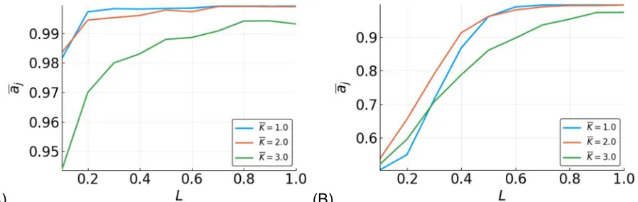
On average, the 3-bit median function is approximated with high accuracy (Fig. S1). All BN RCs perform better than random, with the lowest mean accuracy of ~0.7 for 𝑁= 10, 𝐿= 0.1. Increasing 𝑁 and 𝐿 increases accuracy logarithmically up to ~0.98 for 𝑁= 500, 𝐿= 1 (Fig. 2A). However, reservoirs of size 𝑁 > 200 already have near perfect performance (>0.9) and increasing 𝐿 has a minimal effect in these reservoirs. The general trend in the accuracy in relation to 𝑁 and 𝐿 remains the same for the 5-bit median (Fig. S2). However, the overall accuracy is lower relative to the 3-bit median (Fig. 3A).
The average in-degree,𝐾, of the reservoirs also affects reservoir performance. For the 3-bit case, the performance is clearly reduced for 𝐾= 3, with those reservoirs having the lowest accuracy. 𝐾 = 1 and 2 have similarly high levels of accuracy (Fig. 2A). However, increasing the size of the function window from 3 to 5 creates a more obvious separation between these 𝐾 values (Fig. 3A). Interestingly, for most values of 𝑁 and 𝐿, 𝐾= 2 reservoirs perform the best; however, for higher values of 𝑁 and 𝐿, accuracy for 𝐾= 1 reservoirs is highest. Overall, these results qualitatively agree with previous work by Snyder et al [38,50].
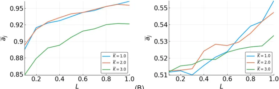
Unexpectedly, when the reservoir is tasked with approximating a 3-bit recursive median, the performance is nearly as high as for the non-recursive 3-bit median and higher than for the 5-bit (non-recursive) median (Fig. 4A). Two notable differences for the recursive median are that (1) increasing 𝐿 does not grant as sharp of an increase in accuracy and (2) the performance of 𝐾 = 3 is more reduced as compared to lower 𝐾 (Fig. S3).
Parity
The accuracy curves for approximating the 3-bit parity function have a strikingly different appearance than those for the median (Fig. 2B). Accuracy is highly dependent on the value of 𝐿, with no reservoir performing better than random (~0.5) for 𝐿 = 0.1. Very small reservoirs
random at 𝐿 < 0.5 and accuracy > 0.8 is only achievable with larger networks (𝑁 > 300) and 𝐿 near 1 (Fig. S2). These observations are consistent with previous work [38,50].
There is not much separation between approximation accuracy curves by values of 𝐾 for the 3-bit parity, though 𝐾 = 3 shows slightly lower performance on the task (Fig. 2B). For the 5-bit parity, reservoirs with different 𝐾 show a clear difference in accuracy (Fig 3B), with 𝐾 = 2 reservoirs being best. As with approximating the median function, accuracy of 𝐾 = 1 reservoirs improves rapidly with 𝐿, changing from lowest to highest accuracy. The relative relationship between the accuracies of different 𝐾-valued reservoirs that we observed is consistent with the above-mentioned previous work, but there are some discrepancies in the actual accuracies observed. We found a much better performance of 𝐾 = 1 and 3 for the 3-bit parity and 𝐾 = 1 and 2 for the 5-bit parity. These differences are likely due to possible differences in how the average in-degree of the reservoir is computed.
The recursive 3-bit parity appears to be extremely difficult to approximate. All reservoirs have an accuracy ~0.5, regardless of 𝑁 and 𝐿, though there is an upward trend in accuracy associated with 𝐿. Interestingly, there is no improvement with increasing 𝑁 and it is unclear whether reservoirs larger than 500 nodes would perform any better. Given the nature of the recursive parity function, it seems that a reservoir would need to “remember” the very first bit of the input signal, which may be too difficult for any reservoir to accomplish.
(A) (B)
Figure 2. Mean accuracy, 𝑎̄, vs. 𝐿 for the 3-bit median(A) and parity(B) functions for different 𝐾-valued reservoirs with 𝑁 = 500.
Figure 3. Mean accuracy, 𝑎̄ , vs. 𝐿 for the 5-bit median(A) and parity(B) functions for different 𝐾 -valued reservoirs with 𝑁 = 500.
(A) (B)
Figure 4. Mean accuracy, 𝑎̄, vs. 𝐿 for the recursive 3-bit median(A) and parity(B) functions for different 𝑲-valued reservoirs with 𝑁 = 500.
Estimating a Range of Functions
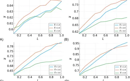
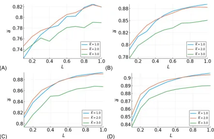
To assess the flexibility of reservoir topologies, all possible 3-bit functions were tested. For each 𝑁, 𝐿 pair, we measured the mean accuracy with respect to all functions and all reservoirs - e.g. 𝑎̄ = ∑ ∑ 𝑎 for 3-bit functions. Similar to what we observed with median and parity functions, 𝐾 = 3 reservoirs show lower performance on the task (Fig. 5).
The observations made in the 3-bit space were clarified in the 5-bit function space. A sample of 5-bit functions showed similar trends as seen in the 3-bit function set, but with greater separation between dynamical regimes (Fig. 6). However, the ability to approximate functions is noticeably lower compared to 3-bit functions. At 𝑁= 100 and 𝐿= 0.5, all prediction accuracies are less than 0.75, regardless of 𝐾. Compared to the performance in the 3-bit function space where accuracy was above 0.95 using similar parameters, in the 5-bit function space, it is not until the parameters are maximized that an accuracy of 0.95 is achieved.
Looking at the effect of 𝐾 in the 5-bit function space, accuracy is increased with 𝑁 and 𝐿 for all 𝐾, but 𝐾 = 2 is most often the most accurate. The accuracy for 𝐾 = 1 is higher than 𝐾 = 2 after certain values of 𝐿. The value of 𝐿 at which 𝐾 = 1 reservoirs outperform 𝐾 = 2 is decreases as 𝑁 increases. This effect is also partially seen in the 3-bit functions (Fig. 5) and 3-bit recursive functions (Fig. 7), though the relationship is less clear, except when looking at specific functions, such as the median and parity (Fig. 3).
(A) (B)
(C) (D)
Figure 5. Mean accuracy, 𝑎̄, vs. 𝐿 for all 3-bit functions for different 𝑲-valued reservoirs. Different sizes of reservoirs are shown: 𝑁 = 10 (A), 𝑁 = 50 (B), 𝑁 = 100 (C), and 𝑁 = 500 (D).
(A) (B)
(C) (D)
(A) (B)
(C) (D)
Figure 7. Mean accuracy, 𝑎̄, vs. 𝐿 for all recursive 3-bit functions for different 𝐾-valued
reservoirs. Different sizes of reservoirs are shown: 𝑁=10 (A), 𝑁 = 50 (B), 𝑁 = 100 (C), and 𝑁= 500 (D).
Reservoir Flexibility
One goal of this work was to assess the flexibility of reservoirs. A highly flexible reservoir can approximate a high number of functions without any changes to the network topology or size. To assess reservoir flexibility, we compute a flexibility metric 𝛷 for each reservoir 𝑖, defined as,
𝛷 = 𝑚𝑒𝑑𝑖𝑎𝑛(𝑎 − 0.5)/𝑚𝑎𝑑(𝑎 ),
where the median and mad (median absolute deviation from the median) are taken over all functions 𝑔 . A reservoir with a low 𝛷 value cannot approximate many (or any) functions well. As the number of functions a reservoir can approximate increases, so does 𝛷.
𝑁 and 𝐿depends on the value of 𝐾 (Fig. S4A,B), though the overall trend remains. For higher values of 𝐾, the transition point towards higher accuracies shifts towards higher values of 𝐿, 𝑁.
The flexibility of reservoirs approximating 5-bit functions is markedly reduced compared to 3-bit functions (Fig. S5A,C,E). For all but the highest values of 𝑁and 𝐿, most reservoirs have only moderate flexibility (𝛷 = 0.25. Unlike for 3-bit functions, the shape of the distributions remain the same across 𝑁 and 𝐿. Consistent with the effect of 𝐾 on mean accuracy, the 𝛷 distributions for 𝐾 = 1 and 𝐾 = 3 are shifted to lower values as compared to 𝐾 = 2.
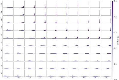
Surprisingly, the distributions of 𝛷 values for reservoirs approximating recursive 3-bit functions behave differently than those of non-recursive 3-bit functions. This was unexpected, since the mean accuracy curves (Fig. 7) for the recursive functions resemble those for the non-recursive functions (Fig. 5). While 𝛷 increases with 𝑁and 𝐿 as it does for non-recursive 3-bit functions, the change in the distributions does not follow the same pattern (Fig. S5B,D,F). For low 𝑁, 𝐿 the distribution of 𝛷 values is wide and becomes increasingly narrow and peaked with increasing 𝑁 and 𝐿, as compared to the narrow peaky edges and flat wide middle of the non-recursive 3-bit 𝛷 distributions.
Figure 8. Histogram of 𝛷 across all 100 reservoirs for each 𝑁, 𝐿 with 𝐾= 2 for 3-bit functions. Each subplot represents the density for all the reservoirs with one 𝑁 and 𝐿, with the x-axis being 𝛷 and the y-axis being number of reservoirs[0,256].
Determinants of Difficulty
approximated that could contribute to lower estimation accuracy. One possible way to compare Boolean functions with the same number of input variables is via the average sensitivity [57,58] of the function, 𝑠̄ . As the name suggests, this metric evaluates how sensitive the output of a function is to any change in the inputs. The average sensitivity of a function 𝑔 is given by
𝑠̄ = 𝐸[𝑠 ([𝑢 , 𝑢 , . . . , 𝑢 ])]
where 𝑠 ([𝑢 , 𝑢 , . . . , 𝑢 ]) = ∑ 𝜒[𝑔([𝑢 , 𝑢 , . . . , 𝑢 ]) ⊕ 𝑒 ≠ 𝑔([𝑢 , 𝑢 , . . . , 𝑢 ])]
and 𝑒 is the unit vector with a 1 in the 𝑖th position and 0s elsewhere and 𝜒[𝐴] is an indicator function that gives a 1 if 𝐴 is true and 0 if 𝐴 is false. The expectation is typically taken with respect to a uniform distribution over the 𝑀-dimensional hypercube.
A function that is insensitive has a low average sensitivity. For example, the constant function, 𝑔([𝑢 , 𝑢 , 𝑢 ]) = 1 , is not dependent on any of its inputs and thus, 𝑠̄ = 0. On the other hand, the 3-bit parity, 𝑔([𝑢 , 𝑢 , 𝑢 ]) = 𝑢 ⊕ 𝑢 ⊕ 𝑢 , has a high average sensitivity as it will take a different value if any of its input variables are toggled, making 𝑠̄ = 𝑀 = 3, the
maximum possible value. The sensitivity can be interpreted as the smoothness of a function. We hypothesized that a function with high sensitivity would be more difficult to estimate because it requires more information about the inputs and is harder to generalize.
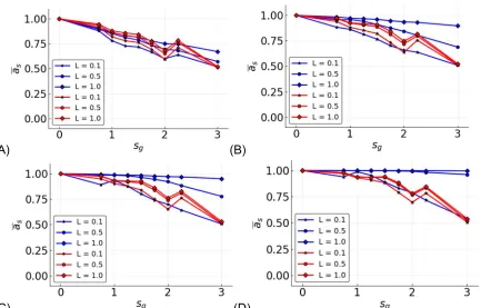
To investigate whether there is a relationship between average sensitivity and accuracy, we computed the average accuracy over all reservoirs approximating all the functions with a given average sensitivity, 𝑎̄ (Fig. 9 and 10). Here, we only discuss results for 𝐾 = 2 since the results for 𝐾 = 1,3 are comparable (Fig. S6). For 3-bit and 5-bit functions there is a clear inverse linear relationship between 𝑠̄ and accuracy. As the average accuracy increases with 𝑁 and 𝐿, the slope of the line becomes less steep, but the relationship remains. Additionally,
approximation of functions with greater 𝑠̄ does not improve as much with larger reservoirs. For low 𝑁, the relationship between sensitivity and accuracy for recursive functions closely matches that for the non-recursive functions. However, as 𝑁 increases, reservoir performance for
recursive functions with high sensitivity remains relatively unimproved.
While the relationship between the average sensitivity and accuracy appears mostly linear, there are clear points of deviation from linearity, most notably at 𝑠̄ = 1, 2, 3, 4. Functions with the same average sensitivities can have different degrees of dependence on each variable. The effect of each variable, 𝑢 , on the output can be measured by the activity, 𝛼 , of that
variable in function 𝑔 [57,59]. The activity of a variable is the probability (hence, 𝛼 is between 0 and 1) that toggling the variable’s value changes the output of the function. If a uniform
distribution of input states is assumed, the sum of the activities is equal to the average sensitivity.
sensitivity of the function, but also the temporal distribution of activities (Fig. 11B). For 5-bit functions, the relationship between accuracy and activities is not as well defined, though still identifiable (data not shown).
Recursive functions behave similarly to non-recursive functions with some exceptions (Fig. S7A,B). Since the recursive variable is the most temporally distant, having high activity on this variable causes an even greater reduction in accuracy. In fact, reservoirs cannot
approximate any recursive functions with 𝛼 = 1. There are also some cases in which reservoirs approximating functions with high activity on the recursive variable have higher accuracy
compared to others with the same sensitivity. It is possible that this is related to the recursive nature of the function.
(A) (B)
(C) (D)
(A) (B)
(C) (D)
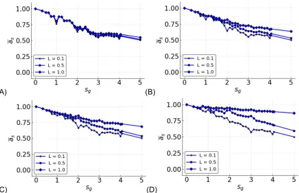
Figure 10. Mean accuracy, 𝑎̄ , vs. function average sensitivity, 𝑠̄ for 5-bit functions. 𝐿 = 0.1 (stars), .0.5(circles), and 1(diamonds) are given in each plot. Four different values for 𝑁 are shown - (A) 𝑁 = 10. (B) 𝑁 = 50. (C) 𝑁 = 100, and (D) 𝑁 = 500. Only reservoirs with 𝐾= 2 are shown.
(A) (B)
Discussion
In this work, we found that the flexibility of a particular BN RC instantiation is a function of the topology and size of the reservoir, encoded by the parameter set (𝑁, 𝐿,𝐾). Generally, higher values of 𝑁 and 𝐿 result in more flexible reservoirs; however, there is heterogeneity when 𝑁 or 𝐿 are low and flexible reservoirs can be found at these values. As noted in research
concerning BN RCs, the optimal parameter set includes tuning the dynamics towards criticality, which leads to more flexible systems. For signal processing, a flexible reservoir will be more accurate and more efficient, requiring less searching and training when different filters are being applied to the same data. For biological systems, where survival is dependent on signal
response, 𝑁, 𝐿, and 𝐾 can be tuned to balance the restraints of the system with the demands of the environment.
In terms of the challenge we provided to the RCs, we found 3-bit functions to be relatively easy to approximate, while 5-bit functions were more difficult, essentially requiring more resources. However 3-bit recursive functions were the most difficult where we noted some recursive functions that are essentially impossible to approximate with this system, likely due to a long memory requirement.
Approximating the 5-bit functions depend on a large reservoir and input size, and more strongly depend on 𝐾. The 5-bit function space is massive, so while we were only able to sample a tiny fraction of it, we clearly saw the effect of dynamics close to criticality on
approximation accuracy. As 𝐾 increased towards chaotic dynamics, the approximation became very poor, leading to large separation between dynamical regimes. Looking forward, it is likely that 7-bit or 9-bit function approximations would require increasingly more resources in terms of reservoir size with more of a dependence on dynamics. This seems to be the case for the median and parity functions, at least [50]. We found that the relative accuracy of reservoirs with 𝐾 = 1, 2, or 3 could change, depending on the value of 𝐿- the input connectivity into the
reservoir. This is most evident with the 5-bit functions in the 𝐾 =2 accuracy plot, which shows a tapering off curve (convex) where improvement with reservoir size is not linear (Fig. 6). In the curves, as 𝐿 increases, we see the 𝐾 = 1 and 𝐾 = 2 accuracy curves crossing each other. One possible explanation for this is that the external perturbations to the reservoir’s nodes shift the dynamics of the reservoir to a less ordered regime - a higher fraction of perturbed nodes resulting in a greater shift. So the dynamics in 𝐾 = 1 approach criticality with higher 𝐿, while the dynamics in the 𝐾 = 2 case moving past criticality, towards chaos, thus dropping in
approximation accuracy. However, the effect of time-varying external perturbation has not been well-studied for Boolean network dynamics. In [50] , it is shown that the mutual information between the reservoir and the signal increase monotonically as 𝐿 increases for 𝐾 = 1, so there may be other effects of increasing 𝐿 at play. Although our results indicate a strong effect of mean in-degree (𝐾) in accuracy, it is possible that accuracy is also affected by other properties of reservoir topology; additional in-degree distributions should be investigated.
if the activities of temporally distant variables are higher. For non-recursive functions, increasing 𝑁 and 𝐿 are sufficient to enable BN RCs to approximate sensitive functions, however, for non-recursive functions, large reservoirs with high values of 𝐿 are not as affected. This points to a large portion of the reservoir needing perturbation to avoid problems related to function argument sensitivity.
However, for recursive functions, even large reservoirs are affected by Boolean function sensitivity. This is likely due to the non-smooth output, which is difficult to approximate. Further, the recursive sliding-window filtering formulation essentially creates infinite memory, albeit fading. Many questions remain, such as what is be needed for good approximations of recursive functions, and whether there is a change to the model that might help. That said, for the most part, many recursive functions are approximated very well, and that may be enough.
Overall, having an idea of the sensitivity of the processing task will inform the minimum parameter values necessary for a successful reservoir. This is intriguing from a biological
standpoint and worth exploring how signal responses that are more sensitive, especially to more historic signal values, are handled. The inability of approximating certain functions may not impinge on the use for modeling biology. When viewed through the lens of 'complex adaptive systems', recursion is a key characteristic, and one that BN RCs would need to address in order to model biological systems.
Conclusion
Reservoir computers with adequately sized Boolean network reservoirs and input sizes show that even a fixed topology is flexible enough to approximate most Boolean functions, applied to signals in a sliding-window fashion, with high accuracy. On one hand, BN RCs have structural similarity to biological systems like gene regulatory networks, while on the other hand, they are useful objects for operating on signals, such as through the application of recursive filters to biological data. We observe that Boolean networks that are closer to the critical dynamics regime lead to more flexible reservoirs. Recursive functions are found to be the most difficult to approximate, owing to the necessity for approximating a function with hidden variables.
Although most recursive functions can be approximated, we find that some can never be approximated. Boolean functions with more arguments are more strongly dependent on the dynamics of the system for accuracy, leading to a greater separation in accuracy curves corresponding to different dynamical regimes. We find a connection between Boolean function sensitivity, an estimate of the smoothness of a function, and the ability to approximate a given function.
Supplementary Materials
Additional figures can be found in the Supplement. Software for constructing and running BN RCs can be found at https://github.com/IlyaLab/BooleanNetworkReservoirComputers.
Acknowledgments
Author Contributions
Conceptualization, M.E. and I.S.; Methodology, D.G., M.N., M.E., and I.S.; Software, M.N., B.A., and D.G.; Validation, M.N., and B.A.; Resources, I.S.; Writing – Original Draft Preparation, M.E. and D.G.; Writing – Review & Editing, M.E., D.G., B.A., I.S.; Visualization, M.E.; Supervision, I.S.; Project Administration, D.G.; Funding Acquisition, I.S.
Conflicts of Interest
The authors declare no conflict of interest.
References
1. Dasgupta S, Stevens CF, Navlakha S. A neural algorithm for a fundamental computing problem. Science. science.sciencemag.org; 2017;358: 793–796.
2. Jaeger H. Adaptive Nonlinear System Identification with Echo State Networks. In: Becker S, Thrun S, Obermayer K, editors. Advances in Neural Information Processing Systems 15. MIT Press; 2003. pp. 609–616.
3. Kitano H. Systems biology: a brief overview. Science. science.sciencemag.org; 2002;295: 1662–1664.
4. Shivdasani RA. Limited gut cell repertoire for multiple hormones. Nat Cell Biol. nature.com; 2018;20: 865–867.
5. Maass W, Natschläger T, Markram H. Real-time computing without stable states: a new framework for neural computation based on perturbations. Neural Comput. 2002;14: 2531– 2560.
6. McCulloch WS, Pitts W. A logical calculus of the ideas immanent in nervous activity. Bull Math Biophys. 1943;5: 115–133.
7. Lu Z, Pathak J, Hunt B, Girvan M, Brockett R, Ott E. Reservoir observers: Model-free inference of unmeasured variables in chaotic systems. Chaos. 2017;27.
doi:10.1063/1.4979665
8. Pathak J, Lu Z, Hunt RB, Girvan M, Ott E. Using machine learning to replicate chaotic attractors and calculate Lyapunov exponents from data. Chaos. 2017;27.
doi:10.1063/1.5010300
9. Fonollosa J, Sheik S, Huerta R, Marco S. Reservoir computing compensates slow
response of chemosensor arrays exposed to fast varying gas concentrations in continuous monitoring. Sens Actuators B Chem. 2015;215. doi:10.1016/j.snb.2015.03.028
10. Caluwaerts K, D’Haene M, Verstraeten D, Schrauwen B. Locomotion without a brain: physical reservoir computing in tensegrity structures. Artif Life. MIT Press; 2013;19: 35–66.
12. Antonelo AE, Schrauwen B, Van Campenhout J. Generative Modeling of Autonomous Robots and their Environments using Reservoir Computing. Neural Process Letters. 2007;26. doi:10.1007/s11063-007-9054-9
13. Bianchi FM, Santis ED, Rizzi A, Sadeghian A. Short-Term Electric Load Forecasting Using Echo State Networks and PCA Decomposition. IEEE Access. ieeexplore.ieee.org; 2015;3: 1931–1943.
14. Gallicchio C, 2014 EAM-FIW, 2014. A preliminary application of echo state networks to emotion recognition. 2011;
15. Gallicchio C, Ia AAM-AA, 2016. A Reservoir Computing Approach for Human Gesture Recognition from Kinect Data. 2013;
16. Waibel A. Modular Construction of Time-Delay Neural Networks for Speech Recognition. Neural Comput. MIT Press; 1989;1: 39–46.
17. Triefenbach F, Jalalvand A, Schrauwen B, Martens J-P. Phoneme Recognition with Large Hierarchical Reservoirs. In: Lafferty JD, Williams CKI, Shawe-Taylor J, Zemel RS, Culotta A, editors. Advances in Neural Information Processing Systems 23. Curran Associates, Inc.; 2010. pp. 2307–2315.
18. Palumbo F, Gallicchio C, Pucci R, Micheli A. Human activity recognition using multisensor data fusion based on Reservoir Computing. J Ambient Intell Smart Environ. 8.
doi:10.3233/AIS-160372
19. Luz EJ da S, Schwartz WR, Cámara-Chávez G, Menotti D. ECG-based heartbeat classification for arrhythmia detection: A survey. Comput Methods Programs Biomed. Elsevier; 2016;127: 144–164.
20. Merkel C, Saleh Q, Donahue C, Kudithipudi D. Memristive Reservoir Computing
Architecture for Epileptic Seizure Detection. Procedia Comput Sci. Elsevier; 2014;41: 249– 254.
21. Buteneers P, Verstraeten D, van Mierlo P, Wyckhuys T, Stroobandt D, Raedt R, et al. Automatic detection of epileptic seizures on the intra-cranial electroencephalogram of rats using reservoir computing. Artif Intell Med. Elsevier; 2011;53: 215–223.
22. Ayyagari S. Reservoir computing approaches to EEG-based detection of microsleeps. University of Canterbury; 2017;
23. Kainz P, Burgsteiner H, Asslaber M, Ahammer H. Robust Bone Marrow Cell Discrimination by Rotation-Invariant Training of Multi-class Echo State Networks. Engineering
Applications of Neural Networks. Springer International Publishing; 2015. pp. 390–400.
24. Reid D, Barrett-Baxendale M. Glial Reservoir Computing. Second UKSIM European Symposium on Computer Modeling and Simulation. IEEE Computer Society; 2008. pp. 81– 86.
26. Yamazaki T, Tanaka S. The cerebellum as a liquid state machine. Neural Netw. 2007;20: 290–297.
27. Dai X. Genetic Regulatory Systems Modeled by Recurrent Neural Network. Lecture Notes in Computer Science. 2004. pp. 519–524.
28. Jones B, Stekel D, Rowe J, Fernando C. Is there a Liquid State Machine in the Bacterium Escherichia Coli? 2007 IEEE Symposium on Artificial Life. 2007.
doi:10.1109/alife.2007.367795
29. Tibshirani R. Regression Shrinkage and Selection via the Lasso. J R Stat Soc Series B Stat Methodol. [Royal Statistical Society, Wiley]; 1996;58: 267–288.
30. Lynn PA. Recursive digital filters for biological signals. Med Biol Eng. 1971;9: 37–43.
31. Burian A, Kuosmanen P. Tuning the smoothness of the recursive median filter. IEEE Trans Signal Process. ieeexplore.ieee.org; 2002;50: 1631–1639.
32. Shmulevich I, Yli-Harja O, Egiazarian K, Astola J. Output distributions of recursive stack filters. IEEE Signal Process Lett. 1999;6: 175–178.
33. Dambre J, Verstraeten D, Schrauwen B, Massar S. Information processing capacity of dynamical systems. Sci Rep. nature.com; 2012;2: 514.
34. Fernando C, Sojakka S. Pattern Recognition in a Bucket. Advances in Artificial Life. Springer Berlin Heidelberg; 2003. pp. 588–597.
35. Kulkarni SM, Teuscher C. Memristor-based reservoir computing. ACM Press; 2009. pp. 226–232.
36. Dale M, Miller JF, Stepney S, Trefzer MA. Evolving Carbon Nanotube Reservoir
Computers. Unconventional Computation and Natural Computation. Springer International Publishing; 2016. pp. 49–61.
37. Kauffman SA. Metabolic stability and epigenesis in randomly constructed genetic nets. J Theor Biol. 1969;22: 437–467.
38. Snyder D, Goudarzi A, Life ACT-, 2012. Finding optimal random boolean networks for reservoir computing. 2009;
39. Derrida B, Pomeau Y. Random networks of automata: a simple annealed approximation. EPL. IOP Publishing; 1986;1: 45.
40. Luque B, Solé RV. Lyapunov exponents in random Boolean networks. Physica A: Statistical Mechanics and its Applications. Elsevier; 2000;284: 33–45.
41. Van der Sande G, Brunner D, Soriano MC. Advances in photonic reservoir computing. Nanophotonics. degruyter.com; 2017;6: 8672.
43. de Jong H. Modeling and Simulation of Genetic Regulatory Systems: A Literature Review. J Comput Biol. Mary Ann Liebert, Inc., publishers; 2002;9: 67–103.
44. Davidich MI, Bornholdt S. Boolean network model predicts cell cycle sequence of fission yeast. PLoS One. 2008;3: e1672.
45. Fumiã HF, Martins ML. Boolean network model for cancer pathways: predicting carcinogenesis and targeted therapy outcomes. PLoS One. 2013;8: e69008.
46. Serra R, Villani M, Barbieri A, Kauffman SA, Colacci A. On the dynamics of random Boolean networks subject to noise: attractors, ergodic sets and cell types. J Theor Biol. 2010;265: 185–193.
47. Helikar T, Konvalina J, Heidel J, Rogers JA. Emergent decision-making in biological signal transduction networks. Proc Natl Acad Sci U S A. 2008;105: 1913–1918.
48. Thakar J, Pilione M, Kirimanjeswara G, Harvill ET, Albert R. Modeling systems-level regulation of host immune responses. PLoS Comput Biol. 2007;3: e109.
49. Damiani C, Kauffman SA, Villani M, Colacci A, Serra R. Cell–cell interaction and diversity of emergent behaviours. IET Syst Biol. 2011;5: 137–144.
50. Snyder D, Goudarzi A, Teuscher C. Computational capabilities of random automata
networks for reservoir computing. Phys Rev E Stat Nonlin Soft Matter Phys. APS; 2013;87: 042808.
51. Bertschinger N, Natschläger T. Real-time computation at the edge of chaos in recurrent neural networks. Neural Comput. 2004;16: 1413–1436.
52. Balleza E, Alvarez-Buylla ER, Chaos A, Kauffman S, Shmulevich I, Aldana M. Critical dynamics in genetic regulatory networks: examples from four kingdoms. PLoS One. 2008;3: e2456.
53. Goudarzi A, Teuscher C, Gulbahce N, Rohlf T. Emergent criticality through adaptive information processing in boolean networks. Phys Rev Lett. 2012;108: 128702.
54. Torres-Sosa C, Huang S, Aldana M. Criticality is an emergent property of genetic networks that exhibit evolvability. PLoS Comput Biol. 2012;8: e1002669.
55. Muñoz MA. Colloquium : Criticality and dynamical scaling in living systems. Rev Mod Phys. 2018;90. doi:10.1103/revmodphys.90.031001
56. Pedregosa F, Varoquaux G, Gramfort A, Michel V, Thirion B, Grisel O, et al. Scikit-learn: Machine Learning in Python. J Mach Learn Res. 2011;12: 2825–2830.
57. Shmulevich I, Kauffman SA. Activities and sensitivities in boolean network models. Phys Rev Lett. APS; 2004;93: 048701.
58. Cook S, Dwork C, Reischuk R. Upper and Lower Time Bounds for Parallel Random Access Machines without Simultaneous Writes. SIAM J Comput. 1986;15: 87–97.