Vortex interactions with topographic features in geophysical fluid dynamics

UCL

Vortex interactions with topographic features in geophysical

fluid dynamics

David C. Dunn

Ph.D. Thesis

1999

Department of Mathematics

University College London

ProQuest Number: 10797842

All rights reserved INFORMATION TO ALL USERS

The qu ality of this repro d u ctio n is d e p e n d e n t upon the q u ality of the copy subm itted.

In the unlikely e v e n t that the a u th o r did not send a c o m p le te m anuscript and there are missing pages, these will be note d . Also, if m aterial had to be rem oved,

a n o te will in d ica te the deletion.

uest

ProQuest 10797842

Published by ProQuest LLC(2018). C op yrig ht of the Dissertation is held by the Author.

All rights reserved.

This work is protected against unauthorized copying under Title 17, United States C o d e M icroform Edition © ProQuest LLC.

ProQuest LLC.

789 East Eisenhower Parkway P.O. Box 1346

A b s tra c t

There are regions in the abyssal ocean where sharp topographic gradients occur, for example escarp­ ments, canyons or seamounts. In such regions the contribution of the topography to the ambient potential vorticity dominates over the ubiquitous effects of planetary curvature, and may play an important part in steering abyssal eddies, such as those affecting the dispersal of newly formed bottom water. This thesis studies some models of vortex motion near a topographic escarpment. The topography produces a restoring mechanism for wave generation, and acts as a wave guide, i.e. the topographic wave phase and energy travels parallel to the isobaths with shallow water on the right in the Northern hemisphere. The ratio, 5, of the time scale for topographic wave generation to the time scale for the vortex circulation, is a measure of vortex intensity. If the two scales axe well separated, i.e. S 1 (a weak vortex) or S < 1 (an intense vortex), analytical progress is made. For a moderate intensity vortex (5 « 1) the wave-vortex interaction is nonlinear and the contour dynamics algorithm is adopted to study the vortex motion in this regime.

In Chapter 1 some examples of geophysical vortices are described, along with their significance. Chapter 2 gives a brief summary of the mathematical preliminaries. Chapter 3 constitutes a review of the relevant work, namely vortex motion over varying topography in quasigeostrophic dynamics. Of interest is vortex motion on the /3-plane, since the methods employed in such studies can be adapted for the present work.

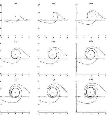
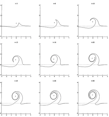
In Chapter 4 the results of McDonald (1998) for the motion of an intense singular vortex near an escarpment are extended to cover the full range of vortex intensities. Analytic results indicate that a weak singular vortex moves parallel to the escarpment in the sense of its image in the escarpment. The vortices which travel in the same direction the phase of the topographic waves radiate waves and experience motion perpendicular to the isobath as a result of energy loss. Numerical results for moderate intensity singular vortices show th a t the motion is characterised by dipole formation. The primary vortex pairs up with an opposite signed patch of relative vorticity which has been produced as a result of cross escarpment advection. An anticyclone located on the shallow side of the escarpment or a cyclone located on the deep side cross the escarpment as a result. A cyclone located on the shallow side of the escarpment or an anticyclone located on the deep side are reflected away from the escarpment.

Chapter 5 is an investigation into the motion of an initially circular vortex patch near an escarpment. It is found th at weak vortex patches behave as if the escarpment were a wall. At large times weak vortices which travel in the same direction as the topographic wave phase radiate wave energy, and are destroyed as a result of topographic wave radiation. Analytical results show th at an intense vortex patch moves in the same manner as an intense /3-plane vortex, i.e. cyclones move along curved northwest trajectories and anticyclones move southwest. Numerical studies for moderate intensity patches show th a t the motion is again characterised by dipole formation.

C ontents

1 I n tr o d u c tio n 5

2 P r e lim in a r y c o n s id e ra tio n s 11

2.1 Shallow water th e o r y ... 11

2.2 Quasigeostrophic m o tio n ... 15

2.3 Quasigeostrophic v o r t i c e s ... 18

2.3.1 Singular vortices on the /-p la n e ... 18

2.3.2 A circular patch of uniform relative v o r t i c i t y ... 20

2.4 Contour d y n a m ic s ... 22

3 Q u a s ig e o s tro p h ic v o rtex-w ave in te ra c tio n s 29 3.1 Vortex motion on the /3-plane... 29

3.2 Vortex motion near sharp potential vorticity g r a d ie n ts ... 33

4 M o tio n o f a s in g u la r v o rte x n e a r a n e s c a rp m e n t 37 4.1 Topographic w a v e s ... 37

4.2 A weak singular v o rte x ... 41

4.2.1 Short time so lu tio n ... 43

4.2.2 Short-time vortex tra je c to ry ... 50

4.2.3 Large-time solution... 54

4.2.4 Large time vortex trajectory ... 62

4.2.5 Contour dynamics r e s u l t s ... 64

4.2.6 Discussion... 69

4.3 An intense singular vortex: a r e v i e w ... 74

4.4 A moderate singular vortex: contour dynamics r e s u l t s ... 77

4.4.1 Anticyclones ... 82

4.4.2 Cyclones... 82

4.4.3 Discussion... 87

4.5 C o n clusions... 92

5 E v o lu tio n o f a n in itia lly c irc u la r v o rte x p a tc h n e a r a n e s c a rp m e n t 95 5.1 Problem fo rm u la tio n ... 96

5.2 A weak vortex p a t c h ... 99

5.2.1 Leading order s o lu tio n ... 100

5.2.2 Contour dynamics r e s u l t s ... 106

5.2.3 Discussion... 120

5.3 An intense vortex p a t c h ... 125

5.3.1 Leading order s o lu tio n ... 126

5.3.2 Contour dynamics r e s u l t s ... 134

5.3.3 Discussion... 137

5.4 Contour dynamics investigations for S « 1... 144

5.4.1 A n tic y c lo n e s ... 145

5.4.2 Cyclones... 145

5.4.3 Discussion... 150

5.5 C o n clusions... 156

6 T h e m o tio n o f a v o rte x n e a r c o a sta l to p o g ra p h y 161

6.1 Linear w a v e s ... 162

6.2 A weak singular v o rte x ...165

6.2.1 Leading order s o lu tio n ... 165

6.2.2 Behaviour a s r - ^ 0 ...168

6.2.3 The quasisteady t e r m ... 169

6.2.4 Large time behaviour ... 171

6.2.5 Vortex tra je c to ry ...179

6.2.6 Contour dynamics r e s u l t s ... 183

6.3 An intense singular v o r te x ... 196

6.3.1 An off shelf v o r t e x ... 196

6.3.2 An on shelf v o r t e x ... 208

6.4 A moderate intensity v o rte x ... 212

6.4.1 An off shelf v o r t e x ... 212

6.4.2 An on shelf v o r t e x ... 222

6.5 C onclusions...222

Chapter 1

Introduction

Many parts of the oceans and atmosphere are characterised by the presence of strong, isolated,

swirling currents, or vortices. These structures exist over a wide range of length scales and axe

often long lived. Whilst it is not on the Earth, the Great Red Spot of Jupiter has become almost

the canonical example of such a vortex in a planetary atmosphere. The Great Red Spot, known

to exist since the invention of the telescope in 1610, was first described by Robert Hooke in 1665,

and continues to swirl to the present day. Figure (1.1) shows a picture of the Great Red Spot taken

in 1979. The Great Red Spot is 14,000 km across in the east-west direction and 40,000 km across

in the north-south direction. It swirls anticlockwise and is located in the upper atmosphere in the

southern hemisphere of Jupiter, which means th at it is an area of high pressure or an anticyclone.

Wind speeds in the Great Red Spot axe up to 360 km/hour.

In 1961 Raymond Hide described the origin of the Great Red Spot in the popular science journal

Nature (Hide, 1961). Unlike fluid which is free to move in three dimensions in an arbitrary way,

the Jovian atmosphere is confined to a thin spherical shell in which vertical velocities axe negligible

compared to horizontal velocities. A remarkable feature of such fluids is the emergence of large

localised laminar vortices from the background small scale turbulent flow (see e.g. McDonald (1999)

and references therein). Figure (1.1) illustrates this well. There axe several (smaller) white vortices

to the south of the Great Red Spot, and the motion in between is rather turbulent. The longevity

of the Great Red Spot is due to opposing shear on the north and south sides, and the rapid rotation

of Jupiter which has a day of length 9.6 hours.

The earth’s atmosphere and oceans shaxe the quasi two-dimensionality of the Jovian atmosphere and

each gives rise to similar isolated vortices. For example, there is the wintertime polar vortex, located

in the stratosphere, and which in effect is isolated from the rest of the atmosphere, enabling the

chemistry of ozone depletion to take place (McIntyre, 1995). Tropical cyclones axe further examples

of intense atmospheric vortices, and which are capable of causing devastation and great cost to

human life.

Vortices are equally prolific in the ocean. They are, for example, produced by instabilities in sepa­

rated intense western-boundary currents. The Gulf Stream is an example of such a current, which

spawns vortices when its meandering becomes sufficiently large. These vortices are lenses of anoma­

lous warm water and axe known as Gulf Stream Rings. Figure (1.2) shows a satellite image of the

sea surface tem perature off the northeast coast of America. The warm Gulf Stream sepaxates from

the western boundaxy of the Atlantic and its meandering motion is evident. Note the warm rings

near the large meander. Gulf Stream rings axe typically a few hundred metres deep and 50 to 200

km in diameter. They move southwest in to the surrounding cold water until they interact with the

shelf or the Gulf Stream itself. Most of the rings have a lifespan of 1-3 months and are eventually

reabsorbed by the Gulf Stream. Similar vortices are shed from the Agulhas current a t the tip of

South Africa and the Kurushio current off the east coast of Japan.

All of the Gulf, Agulhas and Kurushio rings exhibit a strong surface signature. However oceanic

vortices aren’t exclusively surface phenomena. For example the M editerranean salt lenses (meddies)

are large flat discs which form 1000 m below the surface in the Mediterranean sea and move out

into the Atlantic Ocean. Meddies can be 100 km in diameter and about 800 m in vertical extent.

Moreover, they have a lifetime of up to 2 years and travel up to 2000 km into the Atlantic ocean - a

speed of about 2 cm s_1. Recent evidence also suggests th at in the abyssal ocean, deep bottom water

formed in the polar oceans is dispersed by vortices rather than continuous currents (see references

in McDonald (1999)).

One of the most important characteristics of geophysical vortices is their ability to self propagate on

a rapidly rotating planet. Coupled with their longevity this gives vortices the ability to transport

passive scalars, such as momentum, salt, heat and biota, over distances much larger than their

characteristic size. For example the water, in the core of a meddy is up to 4°C warmer than the

surrounding Atlantic water and 1 part per thousand saltier; hence meddies axe responsible for the

dispersal of a large amount of heat and salt throughout the north Atlantic. Similarly Agulhas eddies

transport at least 2.2 x 1020J yr-1 of heat and 14 x 1012kg yr-1 of salt from the Indian ocean to

the Atlantic ocean. Vortices form an important link in the global circulation of the oceans, and

the manner by which they redistribute salt and heat is an im portant factor in determining the

climate and weather. Unfortunately their lengthscales are too small to be resolved by global climate

models and so their effects need to be accurately parametrised in such models. It is of considerable

importance therefore to understand the behaviour of geophysical vortices through simplified models.

Vortices are also important from an environmental point of view. For example the northern ‘wall’

of the Gulf Stream meets the Labrador current which brings a high concentration of phytoplankton

from the nutrient rich polar waters. In turn this provides a happy feeding ground for fish and larger

sea life, and consequently the Nova Scotia and Newfoundland fisheries are rich in marine life. In

addition, the water in the Gulf Stream Rings is not only warmer than the surrounding water, but

the biology is also different. It has been observed th a t springtime blooms occur at different times in

the warm rings than in the neighbouring cold water. Some of the biota present in the rings originate

in the warm Sargasso sea and are not otherwise seen in the cold shelf waters. See Davis and Weibe

(1985). At a smaller scale, surf zone vortices near coastlines may be important in the dispersal of

pollutants.

As alluded to before, geophysical vortices are not simply pushed around by prevailing currents, but

have the ability to self-advect. It is of particular importance to be able to predict the trajectories and

longevity of vortices. This is a complex m atter since planetary rotation, thermodynamics, shearing

currents, neighbouring vortices, friction and bottom topography all contribute to the motion. This

thesis examines the effect of sharp topographic gradients on the motion of vortices. Sharp topography

exists in the deep ocean and may have a considerable effect on the motion of vortices. For example

McDonald (1993) modelled the dispersal of newly formed bottom water from polar regions along

mid ocean ridges by cold eddies. The continental slope affects the trajectories of the Gulf Stream

rings and the Walvis ridge considerably affects the motion of Agulhas rings. Before proceeding with

the study the next chapter presents some of the theoretical background to the present thesis.

Chapter 2

Prelim inary considerations

In this chapter and the next some background theory necessary to the present work is considered

without derivation. The details can be found in Pedlosky (1979), Chapter 3. In chapters 4 through

to 6, quasigeostrophic dynamics of a single layer fluid on an /-plane is modelled. This model ignores

the effects of planetary curvature (usually represented by the /3-plane), which are assumed negligible,

at least locally, compared to the effect of sharp topographic gradients. Vertical structure is trivial,

since it is the dynamics of abyssal eddies th at are of interest, and the deep ocean can be thought of

as a layer of relatively dense fluid lying under an infinitely deep layer of fluid of much lower density.

Future work could include the /3-effect, more general topography or the effects of stratification. Such

work is likely to be numerical in nature. The simple model problems considered in this thesis admit

analytical solutions in certain limits. Moreover, when taken in conjunction with existing analytical,

numerical and experimental studies of vortex-topography interactions it may be possible to identify

some general features of a wide class of geophysical vortex dynamics, an im portant concern for

mesoscale modelling in general circulation models.

2.1

Shallow w ater th eory

In shallow water theory the dynamics of the atmosphere and oceans are modelled by a single “thin”

layer of homogeneous (constant density, p), inviscid fluid, rotating at constant angular velocity ft

about the vertical 2-axis. The motion is governed by the shallow water equations, which in a frame

of reference rotating with the fluid are

lit + (u.V )u + / k A u = - g ' V h (2.1)

Ht + V .(u H ) = 0. (2.2)

The first equation is the momentum equation, and the second is the equation of mass conservation.

Here the dependent variables are u = (u,v), the horizontal velocity of the fluid, and H ( x , y , t ) , the

thickness of the fluid layer. The latter quantity can be written

H(x, y, t) = h(x, y, t) - hB (x, y), (2.3)

where h is the deviation of the free surface from its level position at any point and hB is the equation

of the rigid bottom boundary above some reference level z = 0. The bottom boundary is called the

topography. The independent variables are x, y, the horizontal coordinates, and t the time variable

which has units

Ta = § , (2.4)

where L is the “appropriate” length scale for horizontal motions with corresponding velocity scale

U. Hence Ta is the typical time scale for a fluid particle to move a distance L. In problems involving

vortices, choosing L to be the length scale for the vortex and U to be the typical swirl velocity of the

vortex, Ta is the typical time for a fluid particle to rotate about the vortex centre. For this reason Ta

is sometimes called the eddy turnover time. The remaining quantities in the shallow water equations

are the Coriolis parameter f = 2H, discussed later, and —g'k, the acceleration due to the reduced

gravity of the fluid. In the context of the abyssal ocean the single layer model can be though of as a

layer of relatively dense fluid lying under an infinitely deep less dense upper layer (sometimes called

the l|-la y e r model), where the interface between the layers is free to deform. Then the reduced

gravity is g' = g&p/p, where g is the acceleration due to gravity, p is the fluid density and Ap is the

difference in density between the lower layer and the infinite upper layer.

The vertical scales in the derivation of the shallow water equations axe D, the typical layer depth

and W , the typical vertical velocity. The notion of a thin layer is made precise by insisting th at

j ; < 1, (2.5)

i.e. the horizontal length scale is much larger than the vertical length scale. Equation (2.5) is the

definition1 of the shallow water model, and it implies th at the vertical acceleration is (D / L)2. Thus

a particle with initially zero vertical velocity maintains a zero vertical velocity to within small values

of order (D / L)2 compared with the horizontal accelerations. The tendency of the motion of a thin

rotating fluid to become strongly aligned with the rotation axis is a famous result, known as the

Taylor-Proudman theorem. Taylor (1923) demonstrated th a t when an obstacle is dragged through

a rotating fluid at right angles to the rotation axis, the column initially above the obstacle moves as

a column with the obstacle. The “Taylor columns” are a feature of thin rotating fluids, and enable

the two dimensional description of the large scale horizontal motions.

The choice of a rotating frame of reference gives rise to an apparent force in the momentum equations,

—/ k A u, known as the Coriolis force. Importantly the Coriolis force acts at right angles to the

direction of the fluid motion, i.e. to the right (left) looking in the direction of the motion in the

northern (southern) hemisphere. On the E arth the local horizontal component of the Coriolis force

is unimportant, at least in the mid latitudes (e.g. Gill (1982)), and the vertical component varies

lineaxly with the sine of the latitude <f>. The Coriolis parameter is

/ = 2Oj5sin0, (2.6)

where fIe = 7.292 x 10-5s-1 is the angular velocity of the earth. Taking a fixed latitude (f>is

equivalent to a tangent plane approximation to the curved surface of the planet, and is called the / -

plane. The /-plane describes well mid-latitude motions with only small meridional (i.e. latitudinal)

variations.

The Coriolis parameter varies with latitude due to the sphericity of the E arth sphericity. Rossby

(1939) developed a model in which the Coriolis parameter varies linearly with latitude in the mid

latitudes. In this model, known as the /3-plane, / is approximated by linearising about some mean

latitude (f>o,

/ = fo + &y-> (2.7)

where fo = 20 sin 0O and y is the coordinate in the latitudinal direction. The param eter (3 measures

the variation of the Coriolis param eter in the latitudinal direction and is given by

20

( 3 =— cos </>o, (2.8)

ro

where ro is the radius of the Eaxth. The value of /3 at, for example 30° N, is 1.9 x 10-13cm-1s- 1 .

The /3-plane model has proved to be very useful in understanding the large scale motion of the

atmosphere and oceans. The motion of vortices on the /3-plane has has attracted considerable

attention, and a review is given in the following chapter. It is shown below th a t the /3-plane

approximation is equivalent to the /-plane approximation with linearly sloping topography, and for

this reason comparison of vortex motion near sharp topographic features with vortex motion on the

/3-plane is made throughout this thesis.

In shallow water theory there is a physical quantity of such importance th a t the governing equations

can be written as a single conservation law. The potential vorticity is

n =

^±L,

(

2

.

9

)

where

dv du ,

( = T y - r x ’ (210)

is the relative (i.e. to an observer in the rotating frame) vorticity, which is aligned with the rotation

axis. The potential vorticity is conserved on fluid columns,

+ (2.11)

D t \ H

where

g ^ J + (

- V )

(212)

is the material or advective derivative, which expresses the rate of change of a scalar quantity

following a fluid element in its evolution. The conservation law, (2.11) states th a t relative vorticity

is generated due to vortex column stretching (i.e. changes in H) in the planetary vorticity field /

as fluid columns move over topographic or Coriolis gradients. This single expression encapsulates

the essence of geophysical fluid dynamics. The ubiquitous acquisition of relative vorticity by the

fluid is characteristic of the large scale motions of the atmosphere and oceans. Potential vorticity

conservation is responsible, for example, for the tendency of sub-inertial frequency (Rossby) waves

to adopt a preferential westward phase velocity, or for strong circulating cyclonic currents to follow

curved northwest paths.2

The motion of fluid in the atmosphere and oceans is approximately in a state of so called geostrophic

balance, i.e. the Coriolis force approximately balances the horizontal pressure gradient. Steady,

linearised shallow water motion has velocity components

• - - lM < " *'

' ■

5 1

* “ >

where 77 is the deviation in the free-surface from its resting value. Thus 77 is a streamfunction for the

flow. Since 77 is proportional to the fluid pressure, the flow is equivalently along the isobars, which

is why the isobars are used as a diagnostic in evaluating the weather.

2.2

Q uasigeostrophic m otion

The small departures of the fluid motion from purely geostrophic flow are of most interest. To

examine these departures the shallow water equations are rescaled, with the assumptions th a t the

free surface deviations and the topographic variations are small with respect to the average layer

depth. The equations are then expanded in a series in the Rossby number

R o = j Z , (2.15)

which is a small parameter, i.e. interest is focused on motions whose time scale is much larger

than the inertial period. Small Rossby number flows in dimensional term s are those th a t evolve

over weeks and months as opposed to hours or days. In the context of vortex motion the Rossby

number is the ratio of the inertial period to the eddy turnover time, and is therefore a gauge of the

importance of rotation on the vortex evolution. In particular if R o is of order unity or less then the

rotation of the E arth plays an im portant role in the vortex motion. Typical values of, for example,

an Aghulas ring at 35° S are / = 8 x 10-5s-1 , U = 50 cm s-1 and L = 80 km, leading to Ro « 0.1

(McDonald (1999)).

The derivation is described in detail in Pedlosky (1979), and leads to the conservation law

w = 0’ (216)

where the conserved quantity,

0 = v 2 V > - ( ^ ) i> + f y + S h B, (2.17)

is the quasigeostrophic potential vorticity in the context of a single layer /3-plane. Here rf) is a

streamfunction for the flow and is proportional to the free-surface deviation or the fluid pressure.

hence the name “quasigeostrophic” . The potential vorticity consists of three parts. First, the term

V 2ip in (2.17) is the relative vorticity. The second term ip is a, contribution due to variations

in the free surface elevation, and the parameter L / Rd is the ratio of the horizontal length scale to

the Rossby (deformation) radius,

Rd = ( 2 -2 0 )

The Rossby radius is a length scale which arises naturally in the derivation of the quasigeostrophic

governing equation. It is the ratio of the gravity wave speed to the Coriolis param eter, and is the

length scale on which the relative vorticity and the surface elevation make equal contributions to the

potential vorticity, or alternatively, the length scale on which the tendency of the surface to become

flat due to adjustment under gravity is balanced by the tendency of the Coriolis effect to deform the

surface. It is of great importance in geophysical fluid dynamics, and its presence in (2.17) defines

a preferential length scale for the motion. In particular, the free-surface effect of the rotating fluid

tends to cause disturbances to decay on distances of the order of the Rossby radius.

These first two terms in (2.17) are due to the relative motion. The remaining term s axe present

independently of the motion and axe therefore called the ambient potential vorticity. The variable

part of the ambient potential vorticity, (3y + S h s consists of the planetary vorticity field and the

topography.3 Gradients in the ambient potential vorticity provide a restoring mechanism for wave

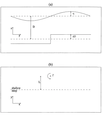
generation. To see this consider the case of h s = sgn(y), and /5 = 0, so th a t y = 0 is an interface

between regions of differing Q, with higher Q lying in y > 0. If this interface is deformed as in

Figure (2.1), the priciple of conservation of potential vorticity implies th a t fluid which has moved

from shallow water to deep water will acquire positive relative vorticity and fluid which has moved

from deep to shallow water will acquire negative relative vorticity. Hence the disturbance propagates

with shallow water (i.e. higher ambient potential vorticity) to the right as shown in Figure (2.1).

It should be noted th a t this ‘stiffness’ of motion in the direction perpendicular to the ambient

potential vorticity gradient is not a consequence of the quasigeostrophic assumption; precisely the

same conclusions can be reached by consideration of the shallow water potential vorticity in equation

(2.9). In fact, the choice of topography mimics the variation of potential vorticity on the /5-plane,

increasing in the poleward direction. Potential vorticity waves on the /5-plane are known as Rossby

shallow

waves

Figure 2.1: The generation of waves by redistribution of ambient potential vorticity. The waves propagate with higher ambient potential vorticity to the right.

waves. Such waves exist whenever there is a gradient in the potential vorticity. Since this occurs

for background sheared currents and variable topography as well as the meridional variation of / ,

potential vorticity waves are ever-present in the atmosphere and oceans.

Furthermore, the swirl velocity of a vortex will cause redistribution of the background potential

vorticity leading to relative vorticity production. The secondary currents associated with this process

will in turn affect the motion and longevity of the vortex - indeed potential vorticity conservation

lends vortices the ability to self propagate. The dimensionless param eter S in (2.17) is a measure of

the strength of this interaction, and can be written as a ratio of tim e scales

Here Ta is the eddy turnover time and $ is the change in the fractional height of the topography

over the horizontal length scale4. Relative vorticity is produced due to vortex column stretching on

the time scale Tw = <5- 1 / -1 , the topographic vortex stretching time and is the time scale on which

this process of wave generation proceeds. For this reason Tw is also called the topographic wave time

scale. Note th at S can also be rewritten

S = ± . (2.22)

In either form 5 describes the relative importance of advection and topographic wave generation.

Both 6 and Ro are small parameters in quasigeostrophic theory, but their ratio S can take on the

whole range of values. In vortex-topography interactions S is a measure of vortex intensity. For

4N ote th at elsewhere in th e text <?() refers the delta-function. T h e m eaning should be clear from th e context.

S <C 1 the vortex is said to be intense, since relative motion due to the swirl velocity of the vortex

dominates over topographic wave generation. For 5 > 1, wave production occurs on a much faster

time scale than advection by the vortex, and the vortex is said to be weak. In these two cases

where the time scales are well separated, leading order solutions to initial value problems are often

available. If, however, S fa 1, then the interaction between the vortex and the waves is nonlinear

and numerical solutions must be sought.

Throughout this thesis it is assumed th a t (3 = 0 and h s ^ 0, i.e. the /3-effect is negligible compared to

the variation in topographic gradients. Of particular interest is the interaction of vortices with sharp

(discontinuous) topographic gradients. In the following section the vortex models to be considered

are presented.

2.3

Q uasigeostrophic vortices

There are two models of vortices used in this work. The first is a singular vortex solution to the

flat bottomed /-plane equations, and the second is a circular patch of uniform relative vorticity.

These two solutions are related in the sense th a t a singular vortex model is often touted as a

good approximation to a uniform patch of relative vorticity. As will be seen this is a reasonable

assumption, at least far from the vortex centre, since both types of vortex have the same velocity

profile in the far-field. From here onwards the unit of length is taken to be the Rossby radius.

2.3.1 Singular vortices on the /-p la n e

Singular vortex solutions appear to have been first obtained by Morikawa (1960). In the absence of

topography {hs = 0 ) and for (3 — 0, the conservation of potential vorticity equation (2.17) implies

(2.23)

where the horizontal length scale has been taken to be the Rossby radius, i.e. L = Rd• To obtain

a singular vortex solution to (2.23), suppose th at at time t — 0, the potential vorticity distribution

where r is the radial distance from the origin. Equation (2.24) is radially symmetric, and away from

the origin is the modified Bessel equation of order zero.

l d _ r dr

1 dip

r dr - i p = 0. (2.25)

The general solution is (e.g. Abramowitz and Stegun (1972))

iP{r) = A K 0(r) + B I 0(r). (2.26)

where Kq and Io are the modified Bessel functions of the first and second kind, zeroth order re­

spectively. Since Iq grows exponentially with its argument, solutions which remain localised must

have B = 0. The coefficient A is determined from the circulation around the origin. The azimuthal

velocity is

v„ = ^ = - A K l (r), (2.27)

where K i is the modified Bessel function of the first kind, first order. Hence the circulation of

velocity around a small circle containing the origin is

r 2 ir r 2 ir

T = — lim

j

J

But, lim K \(r) = 1 /r, so th at

r -» o v '

r 2 n

T = Ade = 2nA t (2.29)

Jo

i.e. A = T/27r. Hence the streamfunction for a singular vortex of strength T at the origin is

m = (2.30)

The sign of T gives the sense of the circulation. For T > 0 it is clockwise (anticyclonic in the

northern hemisphere) and for T < 0 it is positive (cyclonic). The streamlines are circular, and due

to the exponentially decaying nature of the modified Bessel function are bunched near the vortex

centre; this simple vortex model captures the essential effect of the free surface in rotating flows, i.e.

disturbances remain localised, diminishing exponentially on the scale of the Rossby radius5.

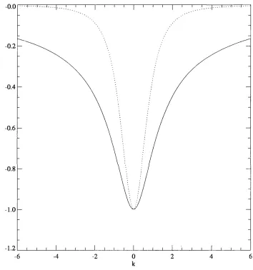
The angular velocity of the vortex is

h(-r) = Vi = & r K liT )■ (2-31)

5It should be noted that a singular vortex violates the quasigeostrophic assum ption since th e am plitud e o f th e free surface deform ation becom es infinite at th e vortex centre. Moreover the horizontal velocities also becom e infinite at th e vortex centre im plying that th e R ossby number is o f th e order o f unity near th e vortex. T hese violation s aren’t considered im portant outside of a sm all neighbourhood of th e vortex.

Figure (2.2) shows a plot of the angular velocity profile of the singular vortex. For r « l , the small

argument form for the modified Bessel functions (e.g. Abramowitz and Stegun (1972)) gives

»(r) * J L , (2.32)

so th at near the origin the quasigeostrophic singular vortex induces the same velocity as the barotropic6

singular vortex of the same strength. On the other hand for large values of r the asymptotic expan­

sions for the modified Bessel functions give, to leading order,

' 2-33>

Thus, the velocity field due to the quasigeostrophic singular vortex decreases exponentially with

distance, on a scale of the Rossby radius, as opposed to the geometric decay in the case of the

baxotropic vortex. Finally, the sign of T is the same as the sign of ip, so cyclones (resp. anticyclones)

correspond to a depression (raising) of the free surface. This is in keeping with oceanic cold (warm)

core rings which are cyclonic (anticyclonic) and have depressed (raised) profiles.

2.3.2

A circular patch of uniform relative vorticity

In the absence of topography (hs = 0), a circular patch of uniform relative vorticity centred at the

origin has

V 2^o — V’o = —otH(a — r), (2.34)

where a is the patch radius, H (z) is the unit Heaviside step function and a gives the sense of the

circulation. For a > 0 it is clockwise (anticyclonic) and for a < 0 it is anticlockwise (cyclonic). The

streamfunction ip0 = ipo(r) is radially symmetric. For r < a equation (2.34) is an inhomogeneous

modified Bessel’s equation of order zero. Solutions which are bounded at the origin have the form

ipo(r) = a ( l 4- A I 0(r)), r < a. (2.35)

For r > a (2.34) is the homogeneous Bessel’s equation of order zero, and has solutions which vanish

in the far-field (i.e. the vortex is localised),

ipo{r) = a B K 0(r), r > a. (2.36)

6T he barotropic approxim ation is obtained by taking Rq —> oo in (2.17), and in th e absence o f topograph y V 2ip =

20

15

10

5

0

0.0 0.5 1.0 1.5 2.0 2.5 3.0

r

Figure 2.2: Profile of the angular velocity, b(r) of a singular vortex with strength r = 1. Note the rapid decay with e-folding length 1, or in dimensional terms, Rd

The constants A and B axe determined by requiring th at ipo and its radial derivative d ^ / d r axe

continuous on the patch boundary r = a. Making use of the Wronskian for the modified Bessel

equations (e.g. Abramowitz and Stegun (1972)),

I n (z)K n+i{z) + I n+1(z)K n (z) = (2.37)

z

the solution is

:s:

m

The angular velocity of the vortex patch, required later is

Kr) = 1 2 * = i ( " “ f " * ° (2.39)

r dr r { —aaIi(a)K i(r), r > a v '

Figure (2.3) show plot of the profiles of the streamfunction and the angular velocity.

The singular vortex is often used as an approximation to a uniform vortex patch. There are two

ways to conceive of this approximation. First, if the motion in the far field is of interest then a

singular vortex with strength T = 2iraali (a) has the same swirl velocity as a circular vortex patch

of radius a. Alternatively,

a 2

lim a a li (a) = a — . (2.40)

a —>0 2

Hence a singular vortex of strength T — ana2 is the solution for a vanishingly small vortex patch.

2.4

C ontour dynam ics

For investigating flows with piecewise-constant distributions of potential-vorticity, a well-known

technique is contour dynamics7, a scheme which integrates the full nonlinear governing equation

(2.17). To derive the algorithm the quasigeostrophic governing equation is recast in a different,

but equivalent form. The following is an adaptation of the derivation by Dritschel (1985) in the

barotropic limit. First, write q = (V2 — 1)^, so th at the potential vorticity is,

Q = q + S hB• (2.41)

Conservation of potential vorticity then leads to the inhomogeneous Helmholtz equation at any given

time,

(V2 - 1 )if> = q. (2.42)

0.4

0.2

0.0

-0.2

-0.4

0.0 0.5 1.0 1.5 2.0 2.5 3.0

r

Figure 2.3: Profiles of the streamfunction, ipo{r) (solid line) and the angular velocity, 6(r) (dotted line) for a circular patch of uniform relative vorticity. The particular case shown has patch radius o = l and strength a = —1, i.e. a cyclone.

The Helmholtz operator, (V2 — 1), has the Greens function — Ko(r)/2n, which leads to

^(*'V) = - 5

~:f j

where r 2 = (x — x ') 2 + (y — y')2 and the integral is taken over the entire fluid domain. The velocity

field, u = v = ipx , determined by (2.43) is

u{x,y) = (u,v) =

J J

Next, suppose th at the anomalous potential vorticity, q, is piecewise constant in regions R k which

cover the fluid domain, i.e. q = qk if (x, y) e Rk- Then (2.44) can be written

to it, with R = 0 and P = —Ko(r), and to v with R — —Kq(t) and P = 0 leads to the velocity field

in terms of line integrals,

where Ck is the boundary of Rk, xjt = (Xk,yk) is a point on Ck , and r\ = (z - Xk)2 + (y - J/fc)28.

The Ck are “contours” , enclosing fluid of constant anomalous potential vorticity, and axe material

curves, i.e. no fluid can cross them. It is straightforward to follow the time evolution of the contours

since the velocity at each point on the contours is given by (2.47).

In the present work the topography is an infinitely long escarpment. Suppose th a t the escarpment

is aligned along y = 0, so h s = sgn(y). Consider the flow regions, shown in Figure (2.4). There

are two contours in the problem. The first is the topographic contour, T, which lies along y = 0,

and the second is the advected, material contour A, initially coincident with T, but which deforms

as the flow evolves. At subsequent times the advected contour moves away from its initial position,

at first by advection by the vortex. The flow then consists of the three types of region depicted in

Figure (2.4). Fluid in regions such as (I) originates in deep water, and has crossed the escarpment,

gaining net anticyclonic circulation, and with q = S. Fluid in regions such as (II) originates on the

shallow side of the escarpment, and has q = —S, due to vortex stretching. The g-field is

(2.45)

Applying Stokes theorem,

(2.46)

K 0(rk)dxk, (2.47)

5, in regions (I) —5, in regions (II) 0, elsewhere.

(a)

Q=s

Q=-S

(b)

m

on)

Figure 2.4: The various regions of the flow, (a) Initially the topographic contour and the advected contour coincide along y = 0. The dynamic potential vorticity q = V2^> — ?/>, is zero everywhere, fluid of high ambient potential vorticity lies in y > 0 and th at of low ambient potential vorticity is in

y < 0. Any initial deflection of the advected contour is solely due to the vortex, (b) At subsequent times the fluid may lie in three types of region. In (I), above the topographic contour, but below the advected contour fluid has moved from deep to shallow water and has q = S. Fluid in regions such as (II), below T but above A similarly have q = —S and elsewhere (III) q remains zero.

Only the regions (I) and (II) contribute to the velocity of the fluid. The arrows in Figure (2.4)

indicate the direction of integration around the boundary of the regions, clockwise in regions (I) and

anticlockwise around regions (II). Equivalently

K v) = ^ Ja Ko{r)dxk ~ J K 0(r)dxk, (2.49)

where r is the distance from the point {x,y) to the point (xk, y k) on A or T respectively. There are

three problems under consideration in this thesis, and the contour dynamics algorithm has to be

applied in a different way in each case.

S in g u la r v o rte x

In Chapter 4 the motion of a singular vortex near an escarpment is considered. Since there is no

self-advection of a singular vortex, the vortex centre is treated as a passive particle, and the velocity

field calculated from (2.49). The velocity at each of the contour nodes is due to the integral around

the contours and the velocity due to the vortex centre.

C irc u la r v o rte x p a tc h

In Chapter 5 the motion of an initially circular vortex patch is considered. Now the vortex does

contribute to its advection. Denote the boundary of the vortex by V. Then the velocity field at any

point of either V or T is

{u,v) = J ^ K 0(rA)dxk - ^ J ^ K 0(rA )dxk + J K 0(rv )dxk , (2.50)

where r y is the distance from the point on V.

C o a s ta l to p o g ra p h y

In Chapter 6 the motion of a singular vortex near an escarpment running parallel to a plane wall is

considered. To apply the contour dynamics algorithm in this case the velocity field due to the image

of the vortex in the wall and the images, T ' and A', of the topographic and advected contours is

included. The velocity at the vortex is due to its image, and the contours T, A, T ' and A' . The

velocity at the contour nodes has the additional contribution due to the vortex and its image.

During the computational runs the advected contours are represented by a discrete set of nodes and

a cubic polynomial through the nodes. The purpose of this is twofold. First, when time-stepping (by

fourth order Runge-Kutta), the contribution to the integrals for the velocity field between adjacent

nodes is calculated to the first order in the departure from a straight line between the nodes, using

the coefficients of the polynomial. Second, the nodes are redistributed at each time step, the spacing

being determined by a non-local node density function, which depends on developing curvature and

velocity. The nodes are then placed at appropriate positions on the cubic polynomial curve. Surgery

is carried out at a predetermined cut-off scale. Full details of the algorithm are given in Dritschel

(1988). Finally, unlike the case of a seamount (e.g. Davey et. al. (1993)), there is no analytical

result for the integral along the undeflected topographic contour. The contribution to the velocity

field is obtained numerically at each time step, in the same way as th a t of the advected contour.

There are two im portant considerations to make. First, the infinitely long advected contour nec­

essarily has a finite representation during computational runs. Therefore, the contour length must

be chosen such th a t its ends remain undisturbed during the runs. The particular contour length

needed for any given parameter values depends on how localised the initial disturbance remains.

Second, in the analytical considerations in the present work, and th at of McDonald (1998) for the

intense vortex limit, the topography is initialised near a pre-existing vortex. In the contour dynamics

computations a vortex is switched on near a pre-existing contour. However, as will be seen later,

contour dynamics results compare well with analytical results in both the weak and intense limits,

so it is assumed th at this is the case for all parameter values.

The codes were tested in several ways. First the time step was decreased until no discernible

difference in the results occurred. Second, the same procedure was carried out with the spatial

resolution parameter. Third, many of the runs were carried out both with and without surgery. In

all cases the trajectory of the vortex centre with surgery active was identical with the trajectory

obtained without surgery. The saving in the number of contour nodes needed was as much as a

factor of 10 over long runs.

Chapter 3

Quasigeostrophic vortex-wave

interactions

The ubiquity of vortices in quasi two-dimensional fluids and the generation of waves through po­

tential vorticity conservation makes vortex-wave interaction a subject of importance in geophysical

fluid dynamics. As pointed out in the introduction vortices are important in the general circulation

of the ocean, but their effects have to be paxameterised in general circulation models. Considerable

attention has been paid to their study through laboratory experiments, numerical studies and the­

oretical investigations. In this chapter a brief review is given of some of the literature relevant to

this thesis.

3.1

V ortex m otion on th e /?-plane

The study of the motion of potentially highly destructive tropical cyclones has motivated much of

the research into vortex motion in the atmosphere. These structures axe intensive, long lived and

have a size comparable to the Rossby radius. Planetary curvature is a leading influence on the

trajectory of a tropical cyclone, and consequently the motion of intense cyclones on the /5-plane

has received considerable attention. The theory of Gulf stream rings has also followed this line of

study. A review of some1 of the literature is presented here. The work has followed two distinct

routes: initial value problems and solitary wave models. This review focuses on the former approach,

i.e. the evolution of an initially circular vortex under the /5-effect. There axe two reasons for this.

First, the techniques employed in /5-plane vortex problems are adopted in the present work. Second,

*It w ould take dozens of pages to sim p ly cite all of th e work!

as described previously, the /3-plane is equivalent to linear sloping topography and it is of interest

to compare the response of a vortex near a sharp topographic gradient with th a t of a vortex over

smooth topography.

The evolution of a weak vortex on the /3-plane is well understood. Flierl (1977) used linear quasi-

geostrophic theory to show th at a weak localised disturbance moves west under the influence of /3

and decays rapidly due to Rossby wave radiation. The decay is substantially slower for more intense

vortices. Laboratory experiments by Firing and Beardsley (1976), and numerical investigations by

McWilliams and Flierl (1979) and Mied and Lindeman (1979) show th at a highly nonlinear (i.e. an

intense) vortex decays slowly and its westward drift speed approaches the Rossby long wave speed.

The effect of nonlinearity is to increase the longevity of the vortex, and to induce meridional motion.

These early studies revealed the first stage of the evolution of an intense vortex under the influence

of /3. The studies of McWilliams and Flierl (1979) and Mied and Lindeman (1979) both showed

th at an intense cyclone (resp. anticyclone) with an initially Gaussian vorticity distribution, follows a

curved northwest (southwest) trajectory. The physical mechanism for this process is well understood.

Consider the case of a cyclone. The sense of the circulation implies th a t fluid lying to the east of

the vortex is advected north, and by virtue of potential vorticity conservation gains anticyclonic

relative vorticity. To the west of the vortex, fluid advected south gains cyclonic relative vorticity.

Thus initially, a dipolar secondary circulation is set up by the primary vortex sweeping fluid columns

across the potential vorticity gradient. The sense of this dipole, the so-called /3-gyres2, is such as

to initially induce a northward motion in the vortex. In the case of the weak vortex Rossby wave

production dominates and energy is rapidly radiated away from the vortex, which in tu rn decays.

In the case of an intense vortex the strong axisymmetric swirl of the vortex dominates the near

field dynamics and the /3-gyres remain in the vicinity of the vortex. In turn the axisymmetric swirl

of the vortex rotates the axis of the dipolar /3-gyres and consequently the vortex follows a curved

northwest trajectory. The case of an anticyclone is analogous, but with the exception th at the

motion is southwest.

Analytical expressions have been found for the /3-gyres in certain cases, and importantly the evolution

of the initially symmetric dipole has been described. Sutyrin and Flierl (1994) considered the

evolution of an initially axisymmetric vortex of piecewise constant potential vorticity using the

quasigeostrophic /3-plane model. Azimuthal mode-1 (i.e. the /3-gyres) is mainly responsible for the

motion of the vortex and in this case an expression for the drift of the vortex centre was obtained.

The initial symmetric disturbance evolves into a uniform westward stream at large times and the

vortex drift speed approaches the Rossby long wave speed. Similar expressions were obtained by

Reznik and Dewar (1994) investigating the dynamics of an initially circular vortex with arbitrary

distribution of relative vorticity with zero circulation using a barotropic /3-plane model, and also by

Reznik (1992) investigating the motion of singular vortices on the /3-plane.

This early stage of the vortex evolution is well understood. However since the vortex drift velocity

approaches the Rossby long wave limit the question arises as to the possible influence of wave

radiation, or put another way, the effect of the higher order normal modes. Reznik and Dewar

(1994) and Sutyrin e t al. (1994) have shown th at the influence of higher order modes reduces the

vortex amplitude and decelerates its westward drift velocity. Until recently all analytical attem pts

at describing the second stage of the vortex evolution have assumed th a t the vortex tends to some

purely westward quasisteady state with a radiated Rossby wave train in its wake. For example, Flierl

(1984), investigating the motion of an intense warm core ring in a two layer non-quasigeostrophic

model, used a solvability condition on the order one field to determine the time evolution of the

lowest order field. In this model the isolated vortex in the upper layer radiates Rossby waves in the

lower layer. In turn this radiation gives rise to a drag on the vortex, which migrates southward in

response.

Recently Reznik and Grimshaw (1998) have argued against this approach on three counts. First they

claim th a t there is no numerical or laboratory evidence th a t the radiated wave field is quasi-steady.

Indeed, they axgue, th at a non-divergent (barotropic) vortex always has a meridional drift speed

of the same order as the zonal drift speed, and so the establishment of a quasisteady wave wake

is not possible. Second the quasisteady wave wake has infinite energy, which is unphysical, since

the system of vortex and waves conserves energy. In particular the vortex must lose energy to the

radiated waves. Third, no previous theories conserve energy or enstrophy.

Reznik and Grimshaw (1998) present a new theory to remedy this charge. In it they show, through

considering solution to higher order terms in a perturbation series in /3, th a t an intense divergent

(quasigeostrophic) vortex on the /3-plane does adopt a quasisteady state, but th a t this is a non­

radiating state. It is shown th at the leading order solution (the /3-gyres) tends to a uniform westward

flow matching the drift speed of the Rossby waves. This “kills” the /3-effect and the vortex moves

steadily westward adopting a nonradiating state. At the next order the /3-gyres produce a correction

consisting of an axisymmetric component and a quadrupolar component. The quadrupole spreads

out from the central region containing the vortex and has little influence on the vortex motion. The

axisymmetric component is opposite in sign to the primary vortex in the vortex core and opposite

in sign outside of the vortex core. The anticyclonic rotation of the annulus in tu rn advects the

planetary vorticity in the opposite sense to the primary vortex. Thus the correction at the third

order is also dipolar and is termed the “secondary /3-gyres” . Since this term is opposite in sense to

the primary /3-gyres the vortex drift velocity is retarded at large times. The im portant conclusion of

this paper is th at the dipolar component of the secondary circulations controls the vortex drift up

to times when the vortex decays. Since this is a near field effect, it is argued th at far-field radiation

has negligible effect on the dynamics.

A further recent study is a numerical investigation which compliments the theoretical results of

Reznik and Grimshaw (1998), by Lam and Dritschel (1998), who apply the new “contour-advective

semi-Lagrangian” (CASL) algorithm of Dritschel and Ambaum (1998) to the evolution of an initially

circular quasigeostrophic vortex on the /3-plane. In doing so the hitherto highest resolution numerical

simulations to date have been produced. Moreover the dependence of the dynamics on the size and

intensity of the vortex was examined. Two key features are identified. First is the existence of a

region of fluid moving with the vortex, a “trapped zone” . This is consistent with the results of

Sutyrin and Flierl (1994), and is due to the axisymmetric component of the secondary circulation

identified by Reznik and Grimshaw (1998). The trapped zone helps to shield the vortex from the

effect of the radiated Rossby waves. Results confirm the rapid decay of a weak vortex and the

longevity and northwest trajectory of a cyclone. Importantly it was shown th a t moderate intensity

vortices undergo the greatest meridional displacement. The mechanism for this enhanced poleward

motion is identified as a “trailing front” , which is part of the radiated Rossby wave train. To describe

it differently, and to reinforce one of the conclusions of this thesis, the trailing front consists of a

patch of anticyclonic relative vorticity and it is the formation of a dipolar mechanism of comparable

3.2

V ortex m otion near sharp p oten tial vorticity grad ien ts

There are regions of sharp (discontinuous) potential vorticity gradients in the ocean. Currents such

as the Gulf Stream are examples of such flows. Near a jet stream the shear flow forms a potential

vorticity interface with the rest of the flow. Vortices are often formed by pinching off from the jet

stream and the local sheax flow dominates over the /2-effect on these vortices. In the abyssal ocean

there are sharp topographic gradients such as seamounts, escarpments and canyons. These features

similarly dominate over planetary curvature in steering deep ocean eddies.

Hide (1961) showed th at for Taylor columns to exist in flow over a finite height object the ratio

S = 5/ Ro must exceed some critical value. Here 6 is the height of the obstacle expressed as a

fraction of the depth of the fluid. If the obstacle is a topographic feature, then S, referred to as

the Hide parameter in flow over finite height object problems, is the same as the S appearing in

the quasigeostrophic potential vorticity (2.17). A right circular cylinder is often used to model a

seamount. Johnson (1984) considered the topographic waves admissible over a seamount, and found

th a t they cycle clockwise around the obstacle with the frequency of the lowest mode of azimuthal

wavenumber-1. This work was extended by Davey et al (1993) to flow over a seamount in multilayer

flow, using contour dynamics. Importantly when the oncoming flow is sufficiently strong or the

height of the seamount sufficiently low, a vortex is created over the seamount as the flow sweeps

the fluid off the seamount and downstream. Also considered was the capture of incident eddies by

the seamount. McDonald and Dunn (1999) have recently made a preliminary investigation into the

evolution of a vortex patch near a seamount. It was found th at anticyclones tended to form dipoles

with the fluid initially located on the seamount.

The limit th at the seamount has infinite radius is the case of an escarpment. Longuet-Higgins (1968)

derived the wave solutions to the shallow water equations over a topographic escarpment. These

waves have unidirectional phase and group velocities, propagating with shallow water to the right in

the northern hemisphere. The amplitude is maximum over the escarpment, and decays exponentially

with distance on either side. These waves are thus dubbed double Kelvin waves or seascarp waves.

Johnson and Davey (1990) studied the surface adjustment problem in /-plane quasigeostrophic

motion over an escarpment, and also found th at the escarpment acts as a wave guide, the waves

propagating with shallow water to their right.

McDonald (1992) considered the time dependent response of fluid to a source of buoyancy near an

escarpment using /-plane quasigeostrophic dynamics. It was found th a t a wavetube is excited and

grows linearly in time at the group velocity of the long topographic waves. However it was found th a t

the flux of fluid away from the source region is less than the flux of fluid a t the source so eventually

nonlinear effects must become important. Numerical studies showed th a t if the source is located on

the shallow side of the escarpment then eddies are formed which self-propagate due to the presence

of the escarpment. In two further studies the role of the escarpment in steering bottom eddies was

investigated. McDonald (1996) investigated the interaction of a modon, (a dipolar distribution of

potential vorticity), with an escarpment. Linear theory predicts th at when the modon moves within

the range of possible topographic wave phase speeds, a radiated wave train is left in the wake of the

modon. As a result the modon speed and radius decay exponentially. There is also an anomalous

case in which the modon moves at the long wave group velocity, so th a t energy cannot escape from

the vicinity of the modon and the response must eventually become nonlinear. In this case the

evolution of the topographic waves is governed by a forced Kortweg-de Vries equation, which leads

to the same result for the rate of decay of the modon as in the linear theory.

In a further study McDonald (1998) studied the motion of an intense singular vortex near a topo­

graphic escarpment, again using quasigeostrophic /-plane dynamics. The leading order drift velocity

components were found and it was shown th at (if the escarpment is chosen to lie in the east-west di­

rection) an intense cyclone follows a curved northwest trajectory and an anticyclone follows a curved

southwest trajectory, qualitatively the same behaviour as a /3-plane vortex. An im portant difference,

however, is th at the westward drift speed is less than the topographic long wave group speed. The

westward drift speed is intimately related to the distance of the vortex from the escarpment. This

indicates an important difference between the case of the continuous topographic gradient and the

sharp topography considered in this thesis: on the /3-plane there is no meaning in “distance from

the topography” , since the gradient of the topography is constant. It is anticipated th a t there will

be new types of behaviour in vortex interactions near an escarpment. McDonald (1998) found an

expression for the large time response of the vortex by equating the momentum flux of the radiated

waves with the rate of change of momentum of the vortex. If the vortex is within about a Rossby

radius of the escarpment then it migrates south (north) if it is an anticyclone (cyclone). Contour