Short Term International Study For Teachers As A Form of Experiential Learning: A Case Study of American Educators in Turkey

(1)

University of South Carolina

Scholar Commons

Theses and Dissertations

2017

Numerical Analysis Of Phase Change, Heat

Transfer And Fluid Flow Within Miniature Heat

Pipes

Mehdi Famouri

University of South Carolina

Follow this and additional works at:https://scholarcommons.sc.edu/etd Part of theMechanical Engineering Commons

This Open Access Dissertation is brought to you by Scholar Commons. It has been accepted for inclusion in Theses and Dissertations by an authorized administrator of Scholar Commons. For more information, please contactdillarda@mailbox.sc.edu.

Recommended Citation

(2)

N

UMERICAL

A

NALYSIS OF

P

HASE

C

HANGE

,

H

EAT

T

RANSFER AND

F

LUID

F

LOW WITHIN

M

INIATURE

H

EAT

P

IPES

by

Mehdi Famouri

Bachelor of Science Persian Gulf University, 2006

Master of Science

University of Mazandaran, 2008

Submitted in Partial Fulfillment of the Requirements

For the Degree of Doctor of Philosophy in

Mechanical Engineering

College of Engineering and Computing

University of South Carolina

2017

Accepted by:

Chen Li, Major Professor

Jamil Khan, Committee Member

Xingjian Xue, Committee Member

Xinfeng Liu, Committee Member

(3)

ii

(4)

iii

DEDICATION

To my parents, Haj Ali Khan Famouri and Banoo Afzal Biglarbeygi, for their

endless love, support and encouragements without which I would not be who I am, where

I am.

ادها

قیوشت و تیامح ،قشع یارب ،یگیبرلگیب لضفا وناب و یروماف ناخ یلع جاح ،منابرهم ردام و ردپ هب میدقت

نیا متسناوتیمن اهنا نودب هک ناشیاهتنا یب یدرف

ا رد و متسه نونکمه هک مشاب ییاجنی

نونکمه هک مشاب سه

(5)

iv

ACKNOWLEDGEMENTS

With immense pleasure and great respect, I express my whole-hearted gratitude,

deep regards and sincere thanks to my PhD advisors Dr. Chen Li for his invaluable,

thoughtful, and brilliant guidance throughout my PhD study at the University of South

Carolina. His encouragement and support have been the constant source of inspiration ever

since I entered this exciting field of research.

I would like to thank my committee members, Dr. Jamil Khan, Dr. Xingjian Xue

and Dr. Xinfeng Liu for their invaluable advice and help throughout my research.

My sincere appreciation is extended to my co-advisors Dr. Gerardo Carbajal at the

University of Turabo, Gurabo, Puerto Rico and Dr. Mahdi Abdollahzadeh at the University

of Porto, Porto, Portugal for their time and help with my research.

I would like to express my sincere regards and thanks to all of my lab mates,

especially Ahmed AbdulShaheed, GuangHan Huang for their suggestions, constant

encouragement and generous help at all stages of my research work.

Special thanks to my fellow numerical friend, lab mate, lifelong friend, Mostafa

Mobli for all the valuable numerical simulation and real life discussions we had over tea

or other types of leisure activities.

Last but not least, the perpetual support and blessing of my family, which reinforced

my determination throughout my career. Even to think of thanking them is to trivialize all

they have done for me. My profound debt to them therefore, remains silent and

(6)

v

ABSTRACT

Heat pipes with broad applications in thermal systems have the ability to provide

effective heat transport with minimal losses in over reasonable distances due to their

passive nature. Their exceptional flexibility, simple fabrication, and easy control, not to

mention, all without any external pumping power make them especially attractive in

electronics cooling. Heat pipe development is motivated to overcome the need to

presumably manage thermal dissipation in progressively compressed and higher-density

microelectronic components, while preserving the components temperatures to

specification.

Computation of flow and heat transfer in a heat pipe is complicated by the strong

coupling among the velocity, pressure and temperature fields with phase change at the

interface between the vapor and wick. Not to mention, the small size and high aspect ratio

of heat pipes brings their own challenges to the table. In this dissertation, a robust numerical

scheme is employed and developed to investigate transient and steady-state operation of

cylindrical heat pipes with hybrid wick structure for high heat fluxes based on an

incompressible flow model. Despite many existing works, this is accomplished assuming

as few assumptions as possible. The fundamental formulation of heat pipe is developed in

such a way to properly take into account the change in the system pressure based on mass

depletion\addition in the vapor core. The numerical sensitivity of the solution procedure

(7)

vi

reformulating the mathematical equations governing the phase change. Hybrid wick

structure of the heat pipe is modeled accurately to further investigate thermal and vicious novel

wick structures.

A fully implicit, axisymmetric sequential finite volume method is devised in

conjunction with the SIMPLE algorithm to solve the governing equations. ANSYS Fluent

software with the power of User Defined Functions and User Defined Scalars is used to

apply the numerical procedure in coupled system and standard levels. This

two-dimensional simulation can solve for symmetrical cylindrical and flat heat pipes, as well

as three-dimensional flat and non-symmetrical cylindrical heat pipes.

Using this powerful and reliable solver, a comprehensive parameter study is carried

out to study the importance and effects of thermal properties, viscous properties, charging

(8)

vii

LIST OF TABLES

Table 2.1 Applied heat inputs, heat losses, real heat inputs and heat fluxes. ...46

Table 2.2 Average condensation temperatures and heat transfer coefficients for each heat input for Groove, Fully Hybrid and Partially Hybrid heat pipe. ...46

Table 2.3 Different boundary conditions and the corresponding effective thermal conductivities ...47

Table 2.4 Summary of different models of effective thermal conductivity of the grooves for water and ethanol...48

Table 2.5 Inlet velocities, pressure drop and the corresponding permeability ...48

Table 3.1 Domain and cell aspect ratios for the Nr =[20, 8, 8], Nx =74 grid. ...73

Table 3.2 List of under-relaxation factors applied to different variables ...73

Table 3.3 List of types and names of the UDFs used in this study ...74

Table 4.1 Mechanical, thermal, viscous properties etc. ...106

Table 4.2 Names and sizes of each computational grids ...107

Table 4.3 Mechanical, thermal, viscous parameters etc. ...108

Table 4.4 Different cases of different cooling conditions and thermal conductivities ....109

Table 4.5 Mechanical, thermal, viscous parameters etc ...110

Table 4.6 Heating and cooling conditions ...111

Table 4.7 Time constants based on Twall,max and Twall,min for fully hybrid heat pipe ...111

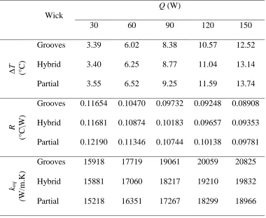
Table 4.8 Total temperature difference, equivalent thermal resistance and equivalent thermal conductivity ...112

Table 4.9 Liquid, vapor and total pressure drop for different wick structures ...113

Table 4.10 Comparison of total pressure drop vs. capillary pressure head ...113

(11)

x

(12)

xi

LIST OF FIGURES

Figure 1.1 Schematic of a heat pipe showing liquid-vapor interface (Ref. [15]) ...18

Figure 1.2 Typical vapor and liquid pressure distribution inside a heat pipe (Ref. [15]) ..18

Figure 2.1 Schematic radial (a) and axial (b) cross sections of the cylindrical heat pipe. .49

Figure 2.2 Schematic view of the cylindrical heat pipe (not-to-scale). ...49

Figure 2.3 (a) Details of the triangular grooves (b) A real

photo of the heat pipe with the triangular helical grooves. ...50

Figure 2.4 (a) Geometric relationship of unit cell [113]

(b) Woven copper screen mesh [116] ...50

Figure 2.5 Schematic of hybrid wick concept (a) Woven coppermesh on top of the copper pillars [116] (b) Micromembrane-enhanced

evaporating surfaces [70] ...51

Figure 2.6 Schematic view of the cross sector of the cylindrical heat pipe (thwall =0.8 mm, thgrv =0.28 mm and thmsh =0.20 mm)

(a) groove wick (rv =5.27 mm) (b) hybrid wick (rv =5.07 mm). ...51

Figure 2.7 Schematics of (a) Groove heat pipe,

(b) Fully Hybrid heat pipe (c) Partially Hybrid heat pipe. ...52

Figure 2.8 Schematic view of the two-dimensional axisymmetric model

(a) Showcase of the grid (b) Showcase of a cell and the velocity components ...52

Figure 2.9 Identical contact area between the cells from different domains

(a) axial grid in two different domains (b) cells from two different domains ...53

Figure 2.10 Thermal resistance modeling of grooves (a) series geometry model, (b) series resistance circuit,

(c) parallel resistance geometry model, (d) parallel resistance circuit ...54

Figure 2.11 Pure heat conduction model to predict the

effective thermal conductivity of the grooves. ...55

Figure 2.12 Temperature distribution showcase of model with

(13)

xii

Figure 3.1 Three computational domains with their grid (a) actual dimensions (b) dimensions in r direction are magnified 10 times (c) dimensions

in r direction in the Vapor domain are magnified 10 times and in

the Wick and Wall domains 100 times. ...75

Figure 3.2 (a) A typical control volume with its neighbors

(b) A typical control volumes from Wick and Vapor domain at their interface ...76

Figure 3.3 A steady-state two dimensional laminar incompressible

test model to compare UDS vs. Temperature at the outflow boundray. ...76

Figure 3.4 Test model to compare the UDS vs. Temperature Results (a) velocity distribution (b) Temperature distribution with U0 =10-6,

(c) UDS distribution with U0 =10-6, (d) Temperature distribution

with U0 =10-5 (e) UDS distribution with U0 =10-5 ...77

Figure 3.5 Bottom wall Temperature and UDS profiles for different inlet velocities. ...78

Figure 3.6 Finding neighboring cells on boundaries at the

interface from different domains ...78

Figure 3.7 Overall Solution Algorithm ...79

Figure 4.1 Fully hybrid cylindrical heat pipe (Q =150 W) transient results: (a) Operating pressure, (b) maximum wall temperature,

(c) interface mass balance and (d) interface mass balance (first 10 second) ...115

Figure 4.2 (a) maximum velocity versus time for different time steps,

(b) wall temperature distributions in 3 different times for different time steps ...116

Figure 4.3 Groove cylindrical heat pipe (Q =150 W) transient results: (a) Operating pressure, (b) maximum wall temperature,

(c) maximum axial velocity (d) interface mass balance

for different grid sizes (listed in Table 1.2) ...117

Figure 4.4 Groove cylindrical heat pipe (Q =150 W) wall temperature

at time = 5 s for different grid sizes (listed in Table 1.2) ...118

Figure 4.5 Cylindrical heat pipe studied by Faghri and Buchko [49] ...118

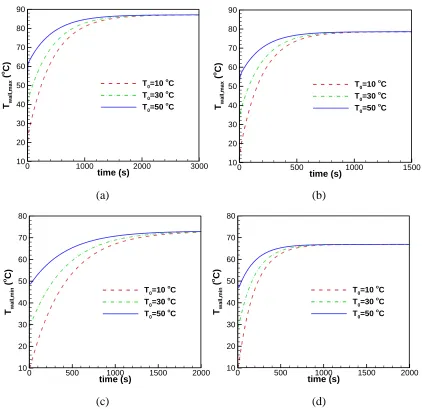
Figure 4.6 Transient operating pressure for different initial conditions

(a) single heater (b) four heaters ...119

Figure 4.7 Transient wall maximum (a and b) and minimum (c and d) temperature for different initial conditions for single heater (a and c)

(14)

xiii

Figure 4.8 Comparison of wall temperature destitutionsbetween

the present work, Faghri and Buchko [49] and Vadakkan [21] ...121

Figure 4.9 Flat heat pipe studied by Vadakkan [49] ...122

Figure 4.10 Comparison of wall temperature distributions

after 20 s and 60s with Ref. [49] ...122

Figure 4.11 Comparison of transient heat output and wall

temperature of evaporation center with Ref. [49] ...123

Figure 4.12 Comparison of (a) Liquid and vapor pressure drop

(b) Operating pressure for 30 W heat input with Ref. [49] ...123

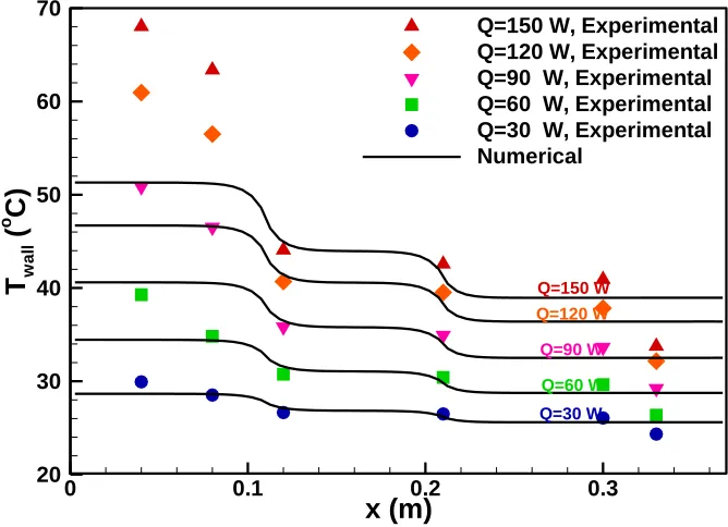
Figure 4.13 Comparison of numerical and experimental

wall temperature distributions for grooves heat pipe ...124

wall temperature distributions for fully hybrid heat pipe ...124

wall temperature distributions for partial hybrid heat pipe ...125

Figure 4.16 Temperature contours of groove (a, c and e) and hybrid (b, d and f) heat pipes for t =1.856 s (a and b), t =5.66 s

(c and d) and t =75.66 s (e and f) for the Q =150 W (Dimensions in r direction in the Vapor domain are

magnified 10 times and in the Wick and Wall domains 100 times) ...126

Figure 4.17 vapor core temperature contours of groove (a, c and e) and hybrid (b, d and f) heat pipes for t =1.856 s (a and b), t =5.66 s (c and d)

and t =75.66 s (e and f) for the Q =150 W. ...127

Figure 4.18 Wall temperature distributions of partially hybrid

cylindrical heat pipe at different times for Q =30 W (a) and Q =150 W (b) ...127

Figure 4.19 Fully hybrid heat pipe maximum (a) and minimum

(b) wall temperatures versus time for different heat inputs ...128

Figure 4.20 Velocity vectors and absolute value contours of groove (a, c and e) and hybrid (b, d and f) heat pipes for t =1.856 s (a and b), t =5.66 s (c and d)

and t =75.66 s (e and f) for the Q =150 W (velocities in wick region are

magnified for groove (1000 times) and hybrid (2000 times) cases) ...129

Figure 4.21 Axial velocity profiles at wick region (at x =0.16 m) for fully hybrid (b and d) and groove (a and c) heat pipes

(15)

xiv

Figure 4.22 The maximum axial velocity of liquid for groove (a) and axial velocity of vapor for groove (b), fully hybrid (c)

and partially hybrid (c) heat pipes for different heat inputs versus time ...131

Figure 4.23 (a) density of liquid and vapor vs. time (b) Product of

average vapor density and maximum vapor velocity vs. time ...132

Figure 4.24 Mass transfer balance at the liquid-vapor interface (Eq. (2.28))

for groove heat pipe versus time for different heat inputs ...132

Figure 4.25 Interfacial mass transfer for groove (a) and partially hybrid

(b) heat pipes versus time for heat input Q = 90 W in different times ...133

Figure 4.26 The zero mass transfer point versus time for different heat inputs for hybrid heat pipe (a) and in heat pipes with different

wick structure for Q =90 W (b) ...133

Figure 4.27 Operating pressure vs. time for different heat inputs ...134

Figure 4.28 Mass of vapor vs. time for different heat inputs ...134

Figure 4.29 Axial vapor pressure distributions along the liquid-vapor interface for groove (a) and (b) partially hybrid heat pipe in

different times for Q =90 W...135

Figure 4.30 Axial liquid pressure distributions along the liquid-vapor interface for groove (a) and (b) partially hybrid heat pipe in

different times for Q =90 W...135

Figure 4.31 Transient liquid pressure drop for different

wick structures and heat inputs ...136

Figure 4.32 Transient vapor pressure drop for partilly haybrid

heat pipe for different heat inputs ...136

Figure 4.33 Dissipated heat from cooling section for groove

heat pipe versus time for different heat inputs ...137

Figure 4.34 Transient maximum wall temperature are depicted

for Q =30 W (a) and Q = 150 W (b) ...138

Figure 4.35 Transient vapor (a) and liquid (b)pressure drops

for different accommodation coefficients (Q =150 W) ...138

Figure 4.36 Steady-state (a) and early t =0.584 s

(16)

xv

Figure 4.37 Temperature difference (a) and equivalent thermal

conductivity of heat pipe for different heat inputs and σ ...139

Figure 4.38 Transient maximum wall temperature for different heat inputs with and without micro-scale effects for fully hybrid (a)

and partial hybrid (b) heat pipe ...140

Figure 4.39 Zero mass transfer point (b) and steady-state

interfacial mass transfer (a) with and without micro-scale effects ...140

Figure 4.40 Temperature difference (a) and equivalent thermal conductivity of heat pipe comparison with and without micro-scale effects ...141

Figure 4.41 Liquid axial velocity profiles at xm=0 =0.16 m for

different cases as listed in Table 4.12 ...141

Figure 4.42 Transient liquid pressure drops for different cases of

permeability values for Q =30 W (a) and Q =150 W (b). ...142

Figure 4.43 Transient liquid pressure drops for groove heat pipe with Q =150 W ...142

Figure 4.44 Local Mach Number on the axisymmetric line for

(17)

xvi

LIST OF SYMBOLS

AE Evaporation sectionarea, m2 AC Condensationsection area, m2 Cp Specific heat, J/kg∙K

CE Ergun's coefficient

Cf comprerssion factor

hfg Latent heat, J/kg

h∞ Coolant heat transfer coefficients, W/m2∙K k Thermal conductivity, W/m∙K

keff Wick effective thermal conductivity, W/m∙K

K wick permeability, m2

LE Evaporation sectionlength, m

LA Adiabaticsectionlength, m

LC Condensationlength of heat pipe, m

M Mesh number, m-1

mi Interface mass flow rate at node i, kg/s∙m

Mw Wick liquid mass, kg

Mv Vapor liquid mass, kg

Nx Number of axial nodes

Nr Number of radial nodes for each domain

(18)

xvii

Pop System pressure, Pa

P0 Reference pressure, Pa

q′′ Input heat flux, W/m2

Q Input heat, W

Qloss Heat loss from the entire heat pipe, W

QOut Heat output from condensation section, W

Qin,real Heat input from evaporation section, W

R Gas constant, J/kg∙K

t Time variable, s

T Temperature variable, o_C

Ti Interface temperature, oC T0 Reference temperature, oC T∞ Coolant temperature, oC th thickness, m

𝑢⃗ Velocity vector, m/s

ux Axial velocity component, m/s

ur Radial velocity component, m/s

x Axial coordinate, m

r Radial coordinate, m

Greek symbols

Δx x-direction width of control volume, m

Δr r-direction width of control volume, m

(19)

xviii

ΔV Volume of a control volume, m3

ρ Density, kg/m3

µ Viscosity, N.s/m2

φ Wick volumetric ratio

σ Accommodation coefficient

Superscripts

0 Old values

* Previous iteration value

Subscripts

l Liquid

grv Grooves

msh Mesh

m Mean value

o Outside

s Solid

v Vapor

wall Wall

(20)

1

CHAPTER 1:

INTRODUCTION

1.1 Background

Heat pipes are used widespread in broad applications since their operation is

generally passive in essence. High heat transfer rates are doable by heat pipes over long

distances, with minimal temperature difference, exceptional flexibility, simple fabrication,

and easy control, not to mention, all without any external pumping power applied. Possible

applications are varied from aerospace engineering to energy conversion devices, and from

electronics cooling to biomedical engineering. Heat pipe development is motivated to

overcome the need to presumably manage thermal dissipation in progressively compressed

and higher-density microelectronic components, while preserving the components

temperatures to specification [1]. For example, according to the report for NASA [2],

reducing one pound of weight on a spacecraft can help save $10,000 US dollars in launch

costs. Also, in terms of a telecommunication satellite, more than a hundred heat pipes are

often required [3]. Many different types of heat pipes are developed in recent years to

address electronics thermal management problems [4-6], solar energy [7-10] as well as lots

of other applications [6, 11-14] and are shown promising results.

Heat pipes could be manufactured as small as 30 μm × 80 μm ×19.75 mm (micro

heat pipes (MHPs)) or as large as 100 m in length [15]. Micro heat pipe concept is first

proposed by Cotter [16] for the cooling of electronic devices. The micro heat pipe is

(21)

2

comparable in magnitude to the reciprocal of the hydraulic radius of the total flow channel

[17]. Typically, micro heat pipes have convex but cusped cross sections (for example, a

polygon), with a hydraulic diameter in range of 10–500 μm [18]. A miniature heat pipe is

defined as a heat pipe with a hydraulic diameter in the range of 0.5 to 5 mm [19]. However,

the concept of micro and miniature heat pipes are not always properly addressed in the

open literature the way mentioned earlier. For example, miniature heat pipes with micro

grooves are sometimes improperly referred to as micro heat pipes [15]. Note, beyond the

size ranges noted earlier, there are additionally other structural differences between micro

and miniature heat pipes. A heat pipe in which both liquid and gas flow through a single

noncircular channel is a true micro heat pipe where the liquid is pumped by capillary force,

on the edges of channel, from the condensation section to the evaporation section [15]. An

array of parallel micro heat pipes are normally mounted on the substrate surface to boost

the area and consequently the heat transfer. Miniature heat pipes can be designed based on

micro axially grooved structure (1D capillary structure), meshes or cross grooves (2D

capillary structure).

The fluid flow, heat transfer and phase change in heat pipes needs to be better

studied in order to improve the designs to costume specific applications and concepts. The

effects of parameters such as thermal conductivity of the wick and wall, thickness of the

wall, wick and vapor core, permeability of the wick, working fluid, operation conditions

etc on the temperature, velocity and pressure distributions in the heat pipe have to be

thoroughly addressed both in transient and steady-state operation to enrich a novel design.

The analysis of the operation and performance of heat pipes has received a lot of attention,

(22)

3

Carbajal [22], Ranjan [23], Issacci [24], Simionescu [25], Sharifi [26], Jiao [27], Chen and

Faghri [28] and Singh [29].

1.2 Fundamentals of Heat Pipe

The operation of a heat pipe [15, 30] is simply explained based on a cylindrical

geometry as an example, as shown in Figure 1.1, however, the shape and size of the heat

pipes can be different. Heat pipes are consisted of a closed container (pipe wall and end

caps), a wick region\structure, and working liquid in equilibrium state with its own vapor.

Most used working fluid choices are water, acetone, methanol, ammonia, or sodium

depending on the operating temperature. The exterior walls of heat pipe are split into three

sections: the evaporator section, adiabatic section and condenser section. Although, a heat

pipe can have no adiabatic section and also could have multiple evaporation and

condensation sections depending on specific applications and design. The heat

implemented to the outside wall of evaporator section is conducted through the wall of heat

pipe first and then the wick region. At the interface of wick and vapor region, working fluid

vaporizes to vapor and flows to the vapor core which increase the pressure of vapor core.

The arisen vapor pressure is the driving force to push the vapor through the heat pipe to

the condenser, where the vapor condenses to liquid flowing back to the wick region,

releasing its latent heat of vaporization. On the other hand, the condensed liquid is pumped

to the evaporation section through the wick region by the capillary pressure formed by the

menisci in the wick structure. With this loop, the heat pipe can continuously carry the latent

heat of vaporization\condensation back and forth between the evaporation and

(23)

4

push the liquid from condensation section to evaporation section, this loop will be

continued [15].

The menisci at the liquid–vapor interface are highly curved in the evaporator

section because the liquid recedes into the wick structures while in the condensation

section, the menisci are close to flat, as shown in Figure 1.1 [15]. The surface tension

between the working fluid and wick structure at the liquid-vapor interface is how the

capillary pressure built and the change in the curvature of menisci along the heat pipe

would vary the capillary pressure along the heat pipe. This capillary pressure gradient

circulates the fluid against the liquid and vapor pressure losses, and adverse body forces,

such as gravity or acceleration. The pressure drop along the vapor core is a results of

friction, inertia and blowing (evaporation), and suction (condensation) effects, while the

pressure drop along the wick region is mainly as a result of friction [15]. The liquid–vapor

interface is not curved at the end of condensation section and that is where can be used as

a zero reference point for hydrodynamic pressure. A typical liquid and vapor pressures

drops are shown Figure 1.2, however, the axial pressure distribution can be different for

the heat pipes with thin vapor core [31].

The maximum local pressure difference is developed near the end of evaporation

section. The maximum capillary pressure should be as equal as or greater than the sum of

the pressure drops in the wick region and vapor core, assuming there is no body forces. If

there is any body forces, such as gravitational force (assuming it works against liquid

pumping), the liquid pressure drop would be higher, meaning the capillary pressure should

(24)

5

normal heat pipe (normal vapor flow rates in the vapor core), the dynamic effects of vapor

flow cause the pressure drop and increase along the heat pipe, as shown in Figure 1.2.

Basically, heat pipe theory deals with fundamentals of hydrodynamic and heat

transfer. Fluid mechanics analysis is adopted to address the liquid and vapor flow (and

pressure drops consequently) and also capillary pressure. Heat transfer is adopted to

analysis the heat applied\removed, conjugate heat conduction in the wall and wick,

evaporation\condensation at the liquid–vapor interface, and forced convection in the both

vapor core and wick region. Fundamentally, one expects to analyze the internal thermal

processes of a heat pipe as a thermodynamic cycle subject to the first and second laws of

thermodynamics [32, 33].

As heat is being applied before the heat pipe reaches steady-state, the system

pressure in the heat pipes increases with time as more evaporation occurs at the

liquid-vapor interface than condensation. Even small changes in the net rate of phase change at

the interface can cause large changes in system pressure since the liquid/vapor density ratio

is large. Then, the interface pressure (also the saturation temperature) changes based on

Clausius-Clapeyron equation as the system pressure changes. The rates of evaporation and

condensation are dependent of the interfacial resistance [34], which itself is function both

the interfacial pressure and bulk pressure. Not to mention, the density of vapor changes

globally with system pressure and locally with temperature using the perfect gas law. These

non-linear relationships however, can cause difficulties in the convergence of numerical

(25)

6

1.3 Summary of Previous Heat Pipe Modeling

Assumptions and formulations play a very crucial role in the heat pipe simulation.

A real simulation of heat pipe takes a lot of work and is almost impossible since

phenomenon in multi scales levels need to be addressed. Some of the general critical

drawbacks\advantages of heat pipe modeling efforts available in the literature are listed in

this section.

1.3.1 Simplified Analytical Solution

Some researchers [35-39] simplified the equations based on many assumptions in

order to be able to solve them analytically. Some of these assumptions are listed as but

not limited to: steady-state, linear temperature profile across the wall and wick structure,

constant saturation temperature at the liquid-vapor interface, predefined velocity

distribution throughout the vapor core, predefined mass transfer pattern at the

liquid-vapor interface, constant liquid-vapor pressure, constant liquid-vapor temperature, negligible viscous

and inertia effects in the wick, constant thermal and viscous properties. Needless to say,

the assumptions are not necessary valid for all the heat pipes geometries. In this study,

none of the above assumptions are made.

1.3.2. Predefined\Assumed Phase Change Pattern

Some heat pipe simulations [35, 38, 40-45] assumed that evaporative length at the

liquid-vapor interface is as a long as evaporation length outside of the heat pipe where the

heat input applies. Also, the condensation at the liquid-vapor interface happens only along

the condensation section outside of the heat pipe where the cooling happens. Moreover, the

condensation and evaporation rates are assumed to be uniform which are calculated purely

(26)

7

pipe, which means it is assumed that 100% of heat is being transferred through phase

change. These set of assumptions is only usable for steady-state modeling however

depending on the problem, it might be a fair estimation or may not be. Some of the factors

involving can be listed as: geometry of condensation and evaporation sections, thickness

of the wick, effective thermal conductivity of the wick, velocity distribution within the

wick, thermal conductivity of the wall and thickness of the wall. In this study, phase change

has been calculated for all the cells at the interface and all the time steps. There is no

assumption either where\when evaporation\condensation occurs, nor the amount of

evaporation\condensation in this study.

1.3.3. Uniform\Constant Vapor Temperature\Pressure

Some of the numerical simulations of heat pipes [40, 46-48] assumed that the

temperature of the vapor core is constant (steady-state) or uniform (transient). Also, the

vapor pressure is sometimes assumed to be constant or uniform. It is clear they are not

necessary accurate assumptions however they might result in satisfactory outcome,

depending on the problem of course. For long heat pipes whereas the vapor core is long,

the axial temperature difference might be crucial. Same thing goes for pressure as part of

the pressure term comes from ideal gas law where pressure is a function of temperature.

Not to mention, for thin vapor cores where the axial hydrodynamic pressure term is not

negligible, the axial pressure difference in the vapor core can play a major role in the

thermal performance of the heat pipe. In this study, both local temperature and pressure are

(27)

8 1.3.4. System Pressure

System pressure in the vapor core is dealt with in different forms in previous studies

whether the simulation is steady-state [28, 49] or transient [50-55] and whether the Navier–

Stokes equations are solved compressible [22, 24, 28, 49-53, 55-59] or incompressible [21,

31, 60-64]. In the case of incompressible fluid flow in the vapor core, system pressure has

to be assumed since the Navier-Stokes equations only include the pressure gradient term

and not the pressure term itself. To the best of the author’s knowledge, all the previous

studies assumed compressible flow except the comprehensive work done by Vadakkan

[21] which also reported\employed by Vadakkan et al. [31, 60, 61], Ranjan et al. [65, 66],

Famouri et al. [63] and Solomon et al. [67]. Also in this study, incompressible formulation

introduced by Vadakkan [21] is properly used to account the system pressure build-up with

time.

1.3.5. Interface Pressure

The evaporation/condensation resistance at the interface are missed by the most

existing publications and based on their methodology, the interface pressure and the system

pressure are the same. Tournier and El-Genk [52] was the first work to incorporate the

interfacial resistance into their formulation however in the form of compressible flow

formulation with constant vapor temperature. Following, Vadakkan [21] was the first heat

pipe incompressible formulation where the interfacial resistance is incorporated into the

model along with temperature change in the vapor core. In this study, Vadakkan’s [21]

(28)

9 1.3.6. Hybrid Wick Modeling

The most important limitation in a heat pipe is the capillary limit which limits the

maximum heat flux (also known as critical heat flux) that a heat pipe can handle before

dry-out. The capillary limit is dependent on wicking capability of the wick structure. Not

to mention, the heat pipe performance and efficiency are also a function of effective

thermal conductivity, evaporative characteristics and also the permeability of the wick.

With the advances in heat pipe technology, new hybrid wick structures [63, 68-72] are

introduced and employed however not enough attempts are made to model them in the heat

pipe. To the best of author’s knowledge, Famouri et al. [63] is the first and only study to

model a hybrid wick structure in a heat pipe, however, the effective viscous and thermal

properties are calculated for the entire wick structure as one homogeneous structure. This

might not be the best approach since different structures of the hybrid wick has its own

characteristics, in the case of screen wire mesh and grooves as the hybrid wick for instance,

the liquid can be pumped through the grooves easier and the screen mesh can enhance the

evaporation and critical heat flux on the other hand. In this study, different structures of

the hybrid wick region are treated differently meaning the wick region is modeled as a

nonhomogeneous porous media.

1.4 Literature Review

There are many analytical and numerical studies on heat pipe based on varieties of

assumptions and problems. They are presented here under different categories based on

(29)

10 1.4.1 Early Works

One of the earliest studies of the vapor flow in heat pipes was published by Cotter

[73], where one-dimensional modeling, laminar, steady-state, incompressible flow were

assumed based on a cylindrical heat pipe application. Later on, Cotter [16] introduced the

idea of micro heat pipe for the first time and suggested the micro heat pipe is suitable where

close temperature control is required. Bankston and Smith [74] parametrically studied the

vapor flow in a cylindrical heat pipe based on a laminar, steady-state, incompressible and

axisymmetric model using finite difference method. Using a steady-state 2D analysis, they

shew that the one dimensional vapor flow model is not able accurately to predict the axial

heat and mass transfer and pressure drop. Vapor flow in a flat heat pipe was investigated

by Ooijen and Hoogendoorn [75] where a laminar, steady-state and incompressible model

were used to study the pressure drop and velocity profile in the vapor core. A gas-filled

heat pipe was studied by Bystrov and Goncharov [76] analytically and experimentally

during start-up and five stages were categorized as: heat-transfer-agent melting to the onset

of intense evaporation, formation of an axial vapor flux, sonic regime, rearrangement to

subsonic regime, and switching to isothermal operation. A transient model was developed

by Costello et al. [77] to model the heat pipe from frozen state through steady-state

conditions. The model included compressible formulation for the vapor core and

incompressible for the liquid in the wick. Pulsed heat pipe startup was studied by Ambrose

et al. [78] and dry-out\rewetting was compared against capillary limit.

1.4.2 Reduced From

The compressible flow of vapor in a heat pipe and in the transient state was

(30)

11

compared with experimental results. Faghri and Harley [80] introduced a transient lumped

heat pipe formulation for different heating and cooling boundary conditions and the results

were reported to be in good agreement with the existing experimental results. A

steady-state closed form solution of cylindrical heat pipe was presented by Zhu and Vafai [38]

based on a non-Daracian transport model for the fluid flow in the wick region and including

incorporating the effects of liquid-vapor coupling. Shafahi et al. [44, 45] developed the

work of Zhu and Vafai [38] to investigate the effects of using nanofluids in a cylindrical

and flat-shaped heat pipes. Predefined mass transfer patterns were assumed for the

liquid-vapor interface in these works (Ref.s [38, 44, 45]). Lefevre and Lallemand [81] introduced

a two-dimensional steady-state coupled thermal and hydrodynamic model to analytically

study flat micro heat pipes in three dimensions. Their method was employed and developed

by Harmand et al. [39] and Sonan et al. [82] to study the transient thermal performance of

flat heat pipes for electronic cooling. The vapor temperature was assumed constant in these

studies (Ref.s [39, 81, 82]) and heat convection terms were neglected. Arab and Abbas [83]

introduced a steady-state reduced-order model to analyze the effects of the thermophysical

properties of working fluids.

1.4.3 Compressible

1.4.3.1 Steady-State

A concentric annular heat pipe has been developed and studied theoretically and

experimentally by Faghri and Thomas [84, 85] to increase the heat capacity per unit length.

Capillary limits and simple incompressible and compressible analysis were presented for

the concentric annular heat pipe. Chen and Faghri [28] numerically solved the

(31)

12

equations for the wick and wall region were solved. They analyzed the effects of single

and multiple heat sources using a compressible, steady-state model. In a similar study but

based on a steady-state model by Faghri and Buchko [49], a cylindrical heat pipe with

multiple heat sources combinations investigated numerically and experimentally which is

later used as a benchmark by most studies on cylindrical heat pipes. Using the same

methodology but in three dimensions, Schmalhofer and Faghri [86, 87] studied

circumferentially heated low temperature cylindrical heat pipe.

1.4.3.2 Transient

The vapor flow in a flat heat pipe is studied by Issacci et al. [56, 57] and Issacci

[24] using a two-dimensional, transient and compressible model. They also reported that

reverse flow can happen in the vapor core at the condensation and even adiabatic sections

for high heat flux. Cao and Faghri [54] presented a transient, two-dimensional,

compressible model based on cylindrical coordinates to analyze a heat pipe with pules heat

inputs however, pure conduction model were used for the wick.. A high-temperature

sodium/stainless steel cylindrical heat pipe was fabricated and tested by Faghri et al. [88,

89] and numerically studied the steady-state and transient responses of the heat pipe. The

rarefied vapor flow were model for the first time by [55] based on a self-diffusion model

to study the startup of a heat pipe from the frozen state based on a compressible, cylindrical

and transient model. Cao and Faghri [55] studied a cylindrical heat pipe startup from frozen

state based on an axisymmetric, cylindrical and compressible model. The heat transfer in

the wall, wick and vapor were solved as a conjugate problem for the first time. A

gas-loaded heat pipe is modeled by Harley and Faghri [90] based on a transient, compressible,

(32)

13

analyzed the noncondensable gas in the heat pipe as a separate entity for the first time.

Tournier and El-Genk [50-53, 91] and Huang et al. [92] developed a compressible model

to numerically study transient performance of cylindrical heat pipe taking into account the

effect of interfacial pressure for the first time. They also modeled the wick as porous media

and included the heat transfer convective terms in the wick for the first time. Carbajal [22]

and Carbajal et al. [58, 59, 93] studied flat heat pipes in two and three dimensions based a

compressible and transient model. They used kinetic theory to calculate the mass transfer

at the interface and took into account the effect of the change in the size of the capillary

radius along the liquid–vapor interface, for the first time based on Young–Laplace

equation. They reported uniform temperature distribution on the cooling side of heat pipe

while the heating side was subjected to a very non-uniform heat flux suggesting their flat

heat pipe as a very good heat spreader.

1.4.4 Incompressible

1.4.4.1 Steady-State

Layeghi and Nouri-Borujerdi [94] and Nouri-Borujerdi and Layeghi [41, 95] studied the

flow in the vapor core and wick in a concentric annular heat pipe using a steady-state

incompressible model. They assumed predefined mass transfer patterns meaning

evaporation and condensation only happen along the heating and cooling surfaces of the

outer walls. Koito et al. [96], numerically investigated the thermal performance of

flat-plate vapor camper based on a steady-state incompressible model. It was assumed that the

entire liquid-vapor has a uniform temperature which was set to be the saturation

temperature at a given pressure. Lu et al. [46] employed the simplified method suggested

(33)

14

with wick column in two dimensions. The liquid-vapor interface was assumed to have

uniform temperature however, this interfacial temperature was calculated based on an

energy balance. A steady-state incompressible model is used by Kaya and Goldak [98]

based on Bai’s work [99] to simulate a cylindrical heat pipe in three dimensions. They did

not assume any predefined mass transfer pattern at the interface however, they assumed a

reference pressure, to calculate the pressure in the vapor core, only based on a guess of

what the saturation temperature of the heat pipe was going to be. Thuchayapong et al. [42]

studied the effects of capillary pressure on performance of a calendrical heat pipe based on

a steady-state incompressible model. The capillary radius along a heat pipe was assumed

to be a simple linear function while they assumed evaporation and condensation only

happen along the heating and cooling surfaces of the outer walls. In a steady-state

incompressible study by Pooyoo [40] in three dimensions, fluid flow and heat transfer was

studied in a cylindrical heat pipe. Uniform temperature was assumed for the vapor core and

the mass transfer at the liquid-vapor interface was predefined based on the evaporation and

condensation lengths on the outside walls. They used a non-Darcy model to model the fluid

flow in the wick region.

1.4.4.2 Transient

Transient behaviors of flat plate heat pipes was investigated by Xuan et al.[48]

using a transient incompressible model however, the entire vapor was assumed to have

uniform temperature and pressure and treated lump model is applied instead of solving for

the vapor core. Not to mention, the convective heat transfer terms were neglected in the

(34)

15

The most comprehensive incompressible model was introduced by Vadakkan [21] taking

into account the interface resistance, temperature distribution in the vapor core, system

pressure, mass depletion\addition in the vapor and wick regions, and variable density while

no predefined mass transfer pattern were assumed. The proposed method is used in both

two-dimensional [31] and three-dimensional [60, 61] flat heat pipes with single and

multiple heat sources to investigate the steady-state and transient performance of the heat

pipe. They also introduced an improved formulation to solve for the system pressure and

interface temperature without which the solver is very unstable for high heat fluxes. Same

numerical procedure followed by Famorui et al. [63] to investigate a polymer-based micro

flat heat pipe with hybrid wicks in transient and state-state conditions. The very

Vadakkan’s model [21] was employed by Solomon et al. [67] to study effects of Cu/water

nanofluid on thermal performance of a screen mesh cylindrical heat pipe and 20% heat

transfer enhancement was reported. Famouri et al. [64] also adopted Vadakkan’s model

[21] to study different wick structures in a cylindrical heat pipe. In order to further increase

the accuracy of Vadakkan’s model [21], Ranjan [23] and Ranjan et al. [100] studied the

wick microstructure effects such as meniscus curvature, thin-film evaporation, and

Marangoni convection in micro scale and incorporated in the heat pipe in macro scale [62,

101]. A simplified transient incompressible model was proposed by Chen at al. [97] to

study the thermal performance of vapor chambers (flat plate heat pipe). The heat transfer

through the wick was assumed linear (only conduction) and uniform temperature was

assumed for the liquid-vapor interface however, they proposed an equation based on a

(35)

16

Same method but in three dimensions was applied to a heat sink embedded with a vapor

chamber by Chen et al. [102] to investigate the effective conductivity of the vapor chamber.

1.5 Objectives of Dissertation

The goals of the present work are to employ and develop a robust numerical method

to study the steady-state and transient performance of high heat flux heat pipes using as

few assumptions as possible. Instead of playing with the thermal and viscous properties,

the goal of this study is to compute them based on the real heat pipe experiments.

Since there is a strong coupling between the phase change at liquid-vapor interface,

pressure, temperature and velocity fields, the numerical techniques to investigate

steady-state and transient operation of heat pipe is very difficult to devise. Sequential

pressure-based methods do not need storage requirement as much as other method and they are

widely used in fluid flow and heat transfer problem, however, sequential procedures like

SIMPLE algorithm [103], can experience difficulties in convergence when solving such

strongly coupled systems of equations. One of the main objective of this study is to employ

and develop a framework based on a sequential solution (SIMPLE algorithm) to design a

stable and accurate computational procedure for heat pipe simulation, in the incompressible

limit. The two key adjustments are: 1- The fundamental formulation of heat pipe is

developed in such a way to properly take into account the change in the system pressure

based on mass depletion\addition in the vapor core. 2- The numerical sensitivity of the

solution procedure on phase change at the liquid-vapor interface are recognized and

effectively handled by reformulating the mathematical equations governing the phase

(36)

17

For the most part, the numerical simulation works have simply been using thermal

and vicious properties for the wick structure of heat pipes without paying much attention

to the background and some studies even played with these properties so they can get better

results. One of the objectives of this study is to analyze the wick structure in details and

use the most accurate models to estimate these properties for the wick. Moreover, hybrid

wick structures are only modeled once however the model was not comprehensive and

could not distinguish the unique features of the hybrid wick. Special attenuation is paid in

this work to use a comprehensive model to predict the behavior of a hybrid wick.

Last but not least, not enough material is published to investigate the effects of each

parameter on performance of heat pipe. Another goal of this work is to analyze the

importance and effects of each parameter on temperature, velocity and pressure results in

heat pipes.

1.6 Organization of Dissertation

The thesis is organized as follows. Chapter 1 introduced the operation of heat pipes,

the previous works available in the literature, and explained the motivation for this study.

Chapter 2 describes the mathematical model used in this work, including the details of the

heat pipe structure, the governing equations, boundary conditions and initial conditions.

Chapter 3 explains the details of numerical methods and tools used to solve the governing

equations described in the previous chapter. Chapter 4 presents the validations process,

results, comparisons and also the parameter study of the heat pipe. Chapter 5 summarizes

(37)

18

Figure 1.1 Schematic of a heat pipe showing liquid-vapor interface (Ref. [15])

(38)

19

CHAPTER 2:

MODEL DESCRIPTION

This chapter shed light on the basics and details of the theories behind the phase

change, heat transfer and fluid flow in heat pipes. The model is explained based on a

two-dimensional cylindrical heat pipe however it can be easily applied to any other problems.

2.1 Problem Description

The schematic and physical representations of the cylindrical heat pipe are depicted

in Figure 2.1 and Figure 2.2. Note, in order to show the details of the problem, this

schematics are not to scale and all the dimensions in r-axis are exaggerated. Schematic

radial and axial cross sections of the cylindrical heat pipe are shown in Figure 2.1 (a) and

Figure 2.1 (b) respectively. The heat pipe chosen to be illustrated in Figure 2.1 consists of

a combination of grooves and a mesh layer as the wick.

The physical dimensions of the two-dimensional cylindrical heat pipe along applied

heat transfer conditions on evaporation and condensation sites have shown in Figure 2.2.

Since the external applied heating and cooling are symmetric, the heat pipe can be modeled

as an axisymmetric problem with the center line of the pipe being the axisymmetric line,

as shown. The heat pipe is separated into three different regions: Wall, Wick and Vapor

domains. The Wall domain is the very wall of the pipe which is made of copper and is

treated as a solid phase. Meanwhile, the grooves on the wall of heat pipe and the screen

mesh (if there is any) are considered as the Wick domain which is treated as a liquid phase

(39)

20

vapor which is treated as an ideal gas. At the external surface of evaporation section, a

uniform heat flux is applied while the condensation section external surface, an ambient

temperature (T∞ =21°C) with an average effective heat transfer coefficient (h∞ =836.63

W/m2.K) are. The wall and wick are made of copper and the working fluid is water. The heat pipe dimensions and other heat transfer parameters are chosen to correspond to an

actual heat transfer experiment. The heat pipe is 370 mm long (LE = 110 mm, LA = 100 mm

and LC = 160 mm) with outside diameter of 12.7 mm (ro = 6.35 mm) and 0.8 mm wall

thickness (thwall =0. 8 mm, rw =5.55 mm).

2.1.1 Applied Heat Transfer

The heat pipe is tested with 5 different heat inputs ranging from 30 W to 150W

applied to the evaporation section with the total area of 4.39×10-3 m2 (AE =2π×ro×LE).

However, because of the heat losses, the real heat input to the heat pipe is slightly less than

the applied heat input, which is listed in Table 2.1 along with the corresponding heat fluxes.

In order to accurately assess the heat loss during the operation of a heat pipe in evaporate

section, as reported by Huang et al.[71], two thermal couples are mounted on the surface

of thermal insulation outer surfaces and one thermal couple is used to measure the air

temperature. The heat loss primarily comes from air convection, thus, the heat loss can

correlated using the temperature difference, area of surface and a heat transfer coefficient.

A set of preliminary experiments have been conducted to predict the heat loss by Huang et

al.[71] based on the heat pipe investigated in this thesis.

A water heat exchanger is used to cool down the heat pipe. The condenser end of

the heat pipe is placed in chamber of the heat exchanger and the gaps around the

(40)

21

the condenser. Water is supplied with a large reservoir tank (thermostatic water source)

and the water mass flow rate is carefully controlled to keep the condenser section

temperature stable. The heat is dumped by flow of 21°C water (T∞ =21°C) over the

condensation section with the total area of 6.38×10-3 m2 (AC =2π×ro×LC). Three different

types of heat pipes are tested and the average condensation teampreature are listed in Table

2.2 for each heat input. The three tpes wich later would be explained in details are: Groove

(type A), Fully Hybrid (type B) and Partially Hybrid (type C).

2.1.2 Wick Structures

The thermal and hydrodynamic performance of passive two-phase cooling devices

such as heat pipes and vapor chambers is limited by the capabilities of the capillary wick

structures employed. The desired characteristics of wick microstructures are high

permeability, high wicking capability and large extended meniscus area that sustains

thin-film evaporation [104]. Micro structures used in the heat pipe investigated in this study are

groove and mesh.

2.1.2.1 Grooves

Axial helical traingular grooves are fabricitaed in the interior wall of the heat pipe

envelope as the wick efficiently pulls condensate back to the evaporator from the cooler

surfaces where working fluid had condensed. Axially grooved heat pipes work best where

gravity is not a factor, e.g., in horizontal configurations or aerospace/satellite applications.

Axial groove heat pipes are very efficient in returning condensate to the evaporation, cost

less to fabricate than heat pipes with conventional wicks and have a long-range heat transfer

capabilities [19, 105-108]. While the permeability of grooved wicks is high, capability in

(41)

22

angel of 50°±5° and height of 0.28 mm (thgrv =0.28 mm) are mounted inside the pipe on

the wall and there are 75±2 grooves in each pipe. More details about the grooves are

depicted in Figure 2.3 (a) while a real photo of the pipe with the helical grooves studied in

this dissertation is shown in Figure 2.3 (b).

2.1.2.2 Screen Mesh

Due to the ease of fabrication and high degree of accuracy with which the various

parameters, such as volumetric porosity and specific surface area can be controlled, layers

of sintered wire screen are often used in commercial applications to provide enhanced heat

transfer or capillary assisted reflow in two-phase systems [67, 109-114]. These layers of

wire screen are routinely used in numerous applications such as porous fins, capillary wick

structures in heat pipes, filling materials and regenerators for Stirling engines, and many

other applications. The woven copper screen mesh used in this study has wire diameter of

56 μm (d =56 μm) and mesh number of 5709 m-1 (M =5709 m-1 =145 inch-1). Detailed geometric relationship of wire dimeter and the mesh number within a unit cell has been

depicted in Figure 2.4 (a) and picture of a real copper screen mesh has been shown in Figure

2.4 (b). Screen mesh wick structure can be one layer or combined of a few layers of screen

mesh. Two layers of screen mesh with compression factor of 0.9 (Cf =0.9) and thickness

0.2 mm (thmsh =2×2×d× Cf) are used as the screen mesh wick structure in the heat pipe

studied in this dissertation.

2.1.2.3 Hybrid Wick

During the capillary evaporation, the counter interactions of flow resistance and

capillary force determine the overall liquid supply and thus, the CHF. Fine copper woven

(42)

23

resistance through the in-plane direction was significantly high [70]. Microgrooves [106,

108] or channels [115] were superior for liquid supply because of the low flow resistance,

but with limited capillarity [108]. The combination of the advantages of single layer

meshes and microchannels (grooves) could lead to a new type of capillary evaporating

surfaces with high capillary pressure and low flow resistance, which would consequently

result in much higher CHF than each individual [70]. This concept of hybrid wick to

enhance the evaporation is illustrated in Figure 2.5 and is studied in Ref.s [63, 68-72, 110,

116, 117].

Schematic view of the cross sector of the cylindrical heat pipe (not-to-scale) with

groove and hybrid wick are depicted in Figure 2.6 (a) and Figure 2.6 (b) respectively. As

previously mentioned, the heat pipe wall thickness is 0.8 mm and the outside radius of the

pipe is 6.35 mm (thwall =0.8 mm, ro =6.35 mmand rw =5.55 mm). With the thickness of

grooves and mesh to be 0.28mm and 0.20 mm respectively, the radiuses of vapor core for

groove and hybrid heat pipe are 5.27 mm and 5.07 mm respectively (thgrv =0.28 mm, thmsh

=0.20 mm, rv,groove =5.27 mmand rv, hybrid =5.07 mm)

With different combinations of screen mesh and grooves in the heat pipe, 3 different

wick structures are developed and studied: Groove (Figure 2.7 (a)), Fully Hybrid (Figure

2.7 (b)) and Partially Hybrid (Figure 2.7 (c)). As for the partially hybrid case, the axial

length of the mesh is considered to be as long as the evaporation length outside the heat

pipe and is only mounted on top the groove at the evaporation site.

2.2 Assumptions

(43)

24

 Both wick and vapor domains are assumed to be at equilibrium state throughout the

process.

 Wick is assumed to be filled only by liquid and the vapor core only by vapor. There

is no two-phase flow rather single phase flow at each domain.

 Fluid flow in both wick and vapor is assumed to be laminar.

 Fluid flow in both wick and vapor is assumed to be incompressible.

 Saturation condition was only assumed at the liquid vapor interface.

 The vapor core is assumed to follow ideal gas law.

 The temperature of the coolant is assumed to be constant at the condensation side

with uniform heat transfer coefficient.

 All the dissipation effects were neglected.

 Liquid and vapor phases are assumed saturated at their corresponding initial

pressure and temperature.

 The operational heat flux distribution is assumed below the critical heat flux.

 Constant material properties are assumed for solid phase.

 Constant material properties are assumed for liquid phase except the density.

 Constant material properties are assumed for vapor phase except the density.

 Partial isotropic and homogenous porous media is assumed. Different constant

permeability, porosity, effective thermal conductivity are assumed for each type of

wick structure.

 The gravity is assumed to have no effects on the heat pipe.

 It is assumed that the tangential component of interface velocity is negligible and

(44)

25

 It is assumed that the vapor flow in the vapor core stays within subsonic limits.

 No-Slip boundary condition is assumed at the wick-wall interface.

 It is assumed that the numerical grid is made in such a way that neighboring cells

at all the interface have the same contact area.

 Bubble generation, bubble size, the onset of nucleate boiling are not analyzed in

this study.

 It is assumed that condensation and evaporation accommodation coefficients have

the same value.

2.3 Governing Equations

The three computational domains of Wall, Wick and Vapor, as shown in Figure 2.2,

are separately solved however they are coupled through boundary conditions at interfaces

between them. In this section, all the equations used in the model are discussed in details.

Since a two-dimensional axisymmetric model is used, the equations are written in

a cylindrical coordinate system however, only longitudinal (x) and radial (r) coordinates

exist and the angular coordinate (θ) and all its correspondents are removed. For example,

the velocity vector (𝑢⃗ ) could originally be composed of 3 components (𝑢⃗⃗⃗⃗ , 𝑢_𝑥 ⃗⃗⃗⃗⃗ , 𝑢_𝑟 ⃗⃗⃗⃗ ) in a _𝜃

cylindrical coordinate system however, it is consisted of only the radial ( 𝑢⃗⃗⃗⃗⃗ ) and 𝑟

longitudinal (𝑢⃗⃗⃗⃗ ) components written as: 𝑥

𝑢⃗ = 𝑢⃗⃗⃗⃗ + 𝑢𝑥 ⃗⃗⃗⃗⃗ 𝑟 (2.1)

Schematic view of the two-dimensional axisymmetric model with a grid is

showcased in Figure 2.8 (a) with radial (r) and longitudinal (x) axes. Moreover, one cell is

(45)

26

(𝑢⃗⃗⃗⃗ , 𝑢𝑥 ⃗⃗⃗⃗⃗ ). Note, there is no grid in angular coordinate (𝑟 θ) and the angle of the sector is only

been shown to illustrate the model and the fact that the volume of cells change in radial (r)

direction regardless of the grid.

Under the above assumptions and model, the governing equations are written as

below.

2.3.1 Continuity Equation

The continuity equation for the Wick and Vapor domains can be written as

𝜑𝜕𝜌

𝜕𝑡 + 𝜕

𝜕𝑥(𝜌𝑢𝑥) + 𝜕

𝑟𝜕𝑟(𝑟𝜌𝑢𝑟) = 0 (2.2)

Where φ, ρ, t and r parameters are porosity (of the wick), density, time and radius

respectively and the ∂ρ/∂t term accounts for the mass addition\depletion in the Wick and

Vapor domains. Also, 𝑢⃗⃗⃗⃗ and _𝑥 𝑢⃗⃗⃗⃗⃗ are the axial and radial component of the velocity, _𝑟

respectively. Note the porosity is 1 (φ =1) for the Vapor domain and the velocity

components (𝑢⃗⃗⃗⃗ , 𝑢_𝑥 ⃗⃗⃗⃗⃗ ) in the _𝑟 Wick domain are the volume-averaged value.

2.3.2 Momentum Equation

The two-dimensional axisymmetric momentum equations in the Wick and Vapor

domains are written as:

𝜕𝜌𝑢𝑥

𝜕𝑡 +

𝜕

𝑟𝜕𝑥(𝑟𝜌𝑢𝑥𝑢𝑥) + 𝜕

𝑟𝜕𝑟(𝑟𝜌𝑢𝑟𝑢𝑥)

= −𝜑𝜕𝑃

𝜕𝑥 +

1 𝑟

𝜕

𝜕𝑥(𝑟𝜇 (2

𝜕𝑢_𝑥

𝜕𝑥 −

2

3(∇. 𝑢⃗ )))

+1

𝑟 𝜕

𝜕𝑟(𝑟𝜇 (

𝜕𝑢_𝑥

𝜕𝑟 +

𝜕𝑢_𝑟

𝜕𝑥)) + 𝑆𝑥

(46)

27 𝜕𝜌𝑢_𝑟 𝜕𝑡 + 𝜕 𝑟𝜕𝑥(𝑟𝜌𝑢𝑥𝑢𝑟) + 𝜕 𝑟𝜕𝑟(𝑟𝜌𝑢𝑟𝑢𝑟) = −𝜑𝜕𝑃 𝜕𝑟 + 1 𝑟 𝜕 𝜕𝑥(𝑟𝜇 ( 𝜕𝑢𝑥 𝜕𝑟 + 𝜕𝑢𝑟 𝜕𝑥)) +1 𝑟 𝜕

𝜕𝑟(𝑟𝜇 (2

𝜕𝑢_𝑟

𝜕𝑟 −

2

3(∇. 𝑢⃗ ))) − 2𝜇 𝑢_𝑟 𝑟2+

2 3

𝜇 𝑟(∇. 𝑢⃗ )

+ 𝜌𝑢𝑥2

𝑟 + 𝑆𝑟

(2.4)

Where μ, Sr and Sxare fluid dynamic viscosity, radial and axial component source

term respectively. Moreover, SrSx and ∇. 𝑢⃗ are as follow:

∇. 𝑢⃗ = 𝜕

𝜕𝑥(𝑢𝑥) + 𝜕

𝑟𝜕𝑟(𝑟𝑢𝑟) (2.5)

𝑆_𝑥= −𝜇𝜑

𝐾 𝑢𝑥−

𝐶_𝐸𝜑𝜌|𝑢⃗ | 𝐾12

𝑢_𝑥 (2.6)

𝑆_𝑟 = −𝜇𝜑

𝐾 𝑢𝑟−

𝐶𝐸𝜑𝜌|𝑢⃗ |

𝐾12

𝑢_𝑟 (2.7)

Where K,CE and |𝑢⃗ | are the Permeability, the Ergun coefficient of the porous media

(Wick domain) and the absolute value of the velocity vector, respectively. Note, the

Permeability is infinity (K =∞) for the Vapor domain which makes the both source terms

zero for the Vapor domain (Sr = Sx =0).

2.3.3 Energy Equation

The two-dimensional axisymmetric energy equations for Wall (Eq. (2.8)), Wick

(Eq. (2.9)) and Vapor (Eq. (2.10)) domains are as follow:

[𝜌𝑐_𝑝]_𝑠𝜕𝑇 𝜕𝑡 = 𝑘𝑠( 1 𝑟 𝜕 𝜕𝑟(𝑟 𝜕𝑇 𝜕𝑟) +

𝜕2_𝑇