Development and Application of a Continuous-Flow Chamber Technique to Measure Nitrous Oxide Emissions from Agroecosystems in the Southeast.

(1)

ABSTRACT

ROSS, NATALIE ALEXANDRA. Development and Application of a Continuous-Flow Chamber Technique to Measure Nitrous Oxide Emissions from Agroecosystems in the Southeast (Under the direction of Drs. Wayne Robarge, Chris Reberg-Horton, and Julie Grossman).

Release of nitrous oxide (N2O) from agricultural soils exhibits temporal and spatial

variability, both of which contribute to uncertainty in quantifying cumulative N2O emissions.

The objective of this study was to decrease uncertainty due to temporal variability in

cumulative N2O emissions estimates from agricultural soils. A robust monitoring system was

used to record an index of the N2O temporal emissions curve in a no-till, conventional

agroecosystem in the Southeast. Quantitative flux measurements were obtained using

non-steady state static chambers. The continuous system operated continuously and unattended in

the field, and it used an infrared gas analyzer (Teledyne® Model T320U) and several

flow-through chambers interconnected via a set of solenoid valves controlled by a microprocessor.

Flow rates were controlled by critical orifices mounted in common manifolds. A laptop

computer running DAQ interface (DAQ Plot®, VVI Software) continuously recorded gas

concentration and sampling location. Individual chambers (n=4) were sampled for 30-minute

intervals. Ambient N2O was measured every 2 hours. During the study period there was only

one peak flux event, during which the bulk of N2O flux occurred. For the remainder of the

season no peak fluxes were observed, though low-levels of N2O flux were detectable. It is

likely that the flux remained low after the peak flux due to drought. Static-chamber flux

measurements were made as soon as possible after rain events and for at least three

consecutive days thereafter. Individual static-chamber flux measurements were calculated

(2)

interpolation of the static-chamber flux measurements and integration under the curve (LII).

The temporal curve from the continuous system was then used to inform adjustments to the

LII approach by defining the start of a flux event (LIIS). For a third approach, N2O flux

decay constants (n=4) were derived from continuous measurements and averaged (RSD =

12.3%). Using the derived decay constant, a simple exponential decay curve was applied to

the static chamber measurements in conjunction with the LIIS approach to estimate

cumulative flux. The cumulative N2O flux values from the LII, LIIS, and LIISD methods

were 1009 ± 827, 609 ± 379, and 768 ± 540 mg N2O m-2, respectively. In this study, the LII

approach over-estimated the cumulative N2O flux as revealed by the temporal pattern in

actual N2O emissions derived from using the flow-through chambers. Correcting the

tendency to over-estimate flux using the LIIS approach by adding in an estimate of the start

in enhanced N2O emissions led to an inherent underestimation in flux because of the time lag

between the start in enhanced N2O emissions and the actual peak in N2O emissions. This

tendency to underestimate cumulative flux using the LIIS approach was corrected with the

LIISD approach by approximating the area under curve following the exponential decline

after the peak in N2O emissions. Improvements in flow-through chamber design will

continue with incorporation of automated, flow-through chambers into the continuous

(3)

(4)

Development and Application of a Continuous-Flow Chamber Technique to Measure Nitrous Oxide Emissions from Agroecosystems in the Southeast

by

Natalie Alexandra Ross

A thesis submitted to the Graduate Faculty of North Carolina State University

in partial fulfillment of the requirements for the degree of

Master of Science

Soil Science

Raleigh, North Carolina

2016

APPROVED BY:

_______________________________ _______________________________

Dr. Wayne Robarge Dr. Julie Grossman

Committee Co-Chair Committee Co-Chair

(5)

DEDICATION

This work is dedicated to all those who seek a deeper understanding of our world and

(6)

BIOGRAPHY

Natalie Ross is an explorer of the world through both science and art. She came to

science by way of an article about mycologist Paul Stamets. The article shared how a simple

oyster mushroom (Pleurotus ostreatus) could transform toxic, diesel-contaminated soil into a

thriving ecosystem, while other remediation efforts of the same soil showed poor to no

results. This simple demonstration of the power of fungi and soil inspired the eternal free

spirit, Natalie, to study our natural world in a formal way. Lucky for her, NCSU was

practically in her backyard and the price was right. Thus, over a decade after starting her

undergraduate career (and after dropping out UNC twice – once to move to San Francisco

and the other time to move to NYC) she graduated from NCSU and loved her alma mater so

much that she decided to stay at NCSU to study soils in a graduate program. Now she’s

emerged from her master’s program, like a butterfly from a cocoon, into the “real world”

with a pocketful of science and a heart full of art. She intends to combine her knowledge of

agriculture with her technology and communication skills to bring the stories of small, local

farmers to the public in a big way. If for some crazy reason you want to talk to her, she can

be summoned by sending a message on the wind. If you don’t know how to do that, then a

(7)

ACKNOWLEDGMENTS

First and foremost I extend my gratitude to Dr. Wayne Robarge for his patient

guidance through this research and writing experience! I’ve enjoyed working with Dr.

Robarge more than I can describe with words. Thank you Dr. Julie Grossman for opening the

door to this research for me and to Dr. Chris Reberg-Horton for keeping the door open.

Of course none of this would have happened without the loving support of my family,

including, but not limited to, my husband, Dr. John Jack, my parents and stepparents, my

sisters, my grandparents and my extended and in-law families. I am so grateful to all of you

for encouragement!

Thank you to all the staff at CEFS who patiently and willingly lent a hand and dealt

with our unconventional field instrumentation. You all rock!

And finally thank you to all the hard-working scientists who paved the way for this

(8)

LIST OF TABLES

Table 1.Total precipitation and descriptive summaries of daily air temperature recorded by NC ECONet Station GOLD-Cherry Research Station, and 10-minute readings of soil temperature and moisture content (depth: 7.62 cm) within the no-till BMP subplot monitored in this project. ... 31 Table 2. Descriptive summary of N2O flux as measured by the non-steady state static

chambers as a function of group for the period April 24, 2015 (DOY 114) to September 3, 2015 (DOY 246). ... 47 Table 3. Cumulative N2O flux (mg m-2 h-1) by static chamber group. Static chamber

cumulative flux was calculated three ways: linear interpolation and integration (LII), LII with the start of the flux event defined (LIIS), and LIIS with a decay curve derived from continuous data and applied to static chamber data (LIISD). ... 64 Table 4. Cumulative N2O flux using non-steady state static chambers in no-till, corn systems fertilized with urea. ... Error! Bookmark not defined. Table A 1. Final nitrous oxide flux calculations from CEFS determined by the HMR method

or linear regression. Flux values were used in analyses in Chapter 2. Flux was measured at ~ noon each day. ... 71 Table C 1. Average N2O concentration in glass vials sealed with red septa presented as

absolute values and as percent of 2000 ppbv N2O over time. Vials (n=10) were filled with 2000 ppbv N2O on day 0, and N2O concentrations were measured for three consecutive days following filling. Values followed by different letters denotes

difference at the p<0.01 level. ... 80 Table D 1. Concentration of N2O in the presence of dissected red rubber septa expressed as

absolute concentration and as percent of 2000 ppbv N2O over time. Vials (n=10) were filled with 2000 ppbv N2O and one dissected septum on day 0, and N2O concentrations were measured for three consecutive days following filling. Values followed by

different letters denotes difference at the p<0.05 level. ... 84 Table E 1. Static chamber measurements were taken 18.63, 42.63, 66.63 and 90.63 hours

after the peak emissions that occurred on May 12, 2015. Peak flux A-values were calculated using static-chamber measurements and the decay curve derived from continuous, flow-through measurements. A-values are shown here as absolute values and as a percent of the calculated A-value from static chamber measurements collected 18.63 hours after the peak. (Units = mg N2O m-2 h-1) ... 87 Table E 2. Comparison of time since peak flux and static chamber flux measurements in

calculating A values using Eq. 3. ... 89

LIST OF FIGURES

Figure 1. State map of North Carolina showing the location of the study site at Goldsboro, NC. ... 29 Figure 2. A map of the study site and diagnostic soils in the FSRU at CEFS in Goldsboro,

(11)

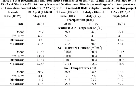
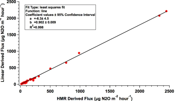
Figure 3. Estimated N2O flux derived using linear regression versus the HMR model for 55% of the observations obtained using the non-steady state static chambers. ... 37 Figure 4. Soil moisture content at 7.62 cm depth and cumulative rainfall for the period April

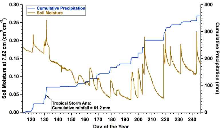
24, 2015 (DOY 114) to September 3, 2015 (DOY 246). ... 44 Figure 5. Ambient air temperature (2m) and soil temperature at 7.62 cm depth for the period

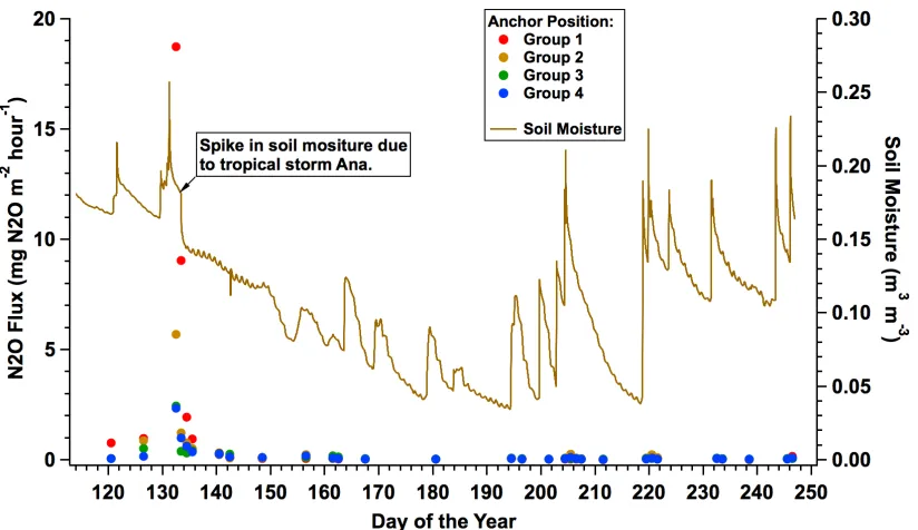
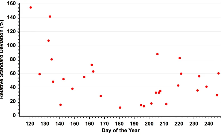
April 24, 2015 (DOY 114) to September 3, 2015 (DOY 246). ... 45 Figure 6. Nitrous oxide flux measured using non-steady state static chambers as a function of group position and soil moisture content as a function of Day of the Year for the period April 24, 2015 (DOY 114) to September 3, 2015 (DOY 246). ... 47 Figure 7. Percent relative standard deviation of individual sets (n=4 chambers per set) of N2O

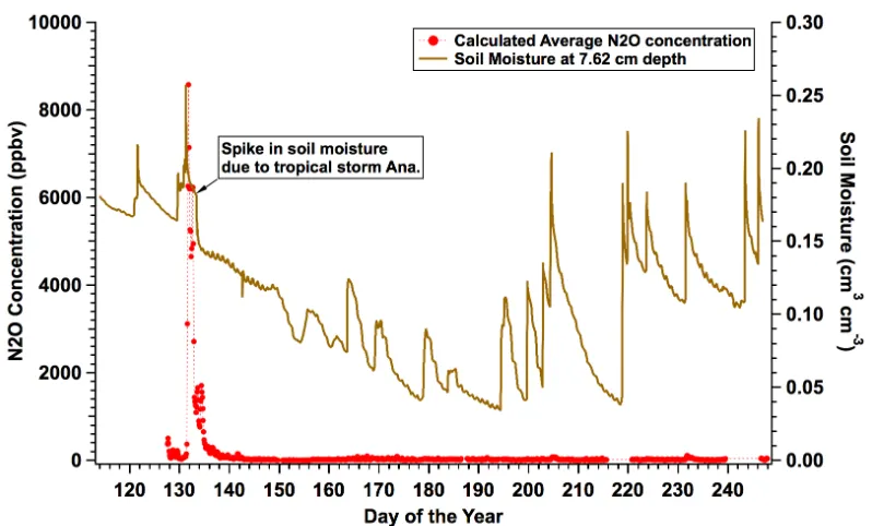
flux measurements using the non-steady state static chambers as a function of Day of the Year for the period April 24, 2015 (DOY 114) to September 3, 2015 (DOY 246). . 48 Figure 8. Net concentration of N2O in headspace of simple flow-through chambers (group 1

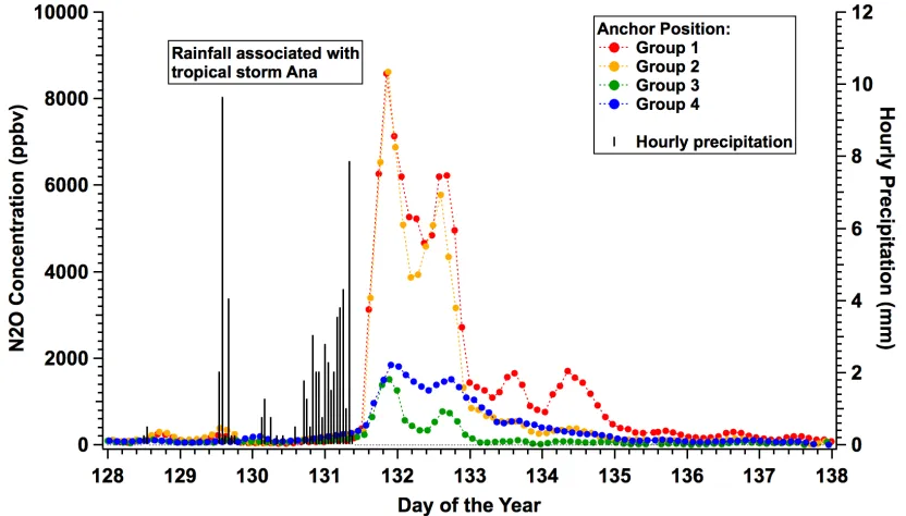
position) and soil moisture content at 7.62 cm depth for period May 5, 2015 (DOY 125) to September 2, 2015 (DOY 245). Dashed line added to aid visual identification of trend between individual data points for N2O concentration. ... 49 Figure 9. Net concentration of N2O in headspace of simple flow-through chambers (groups 1 - 4) and hourly precipitation amounts for the period May 8, 2015 (DOY 128) to May 18, 2015 (DOY 138). Dashed line added to aid visual identification of trend between

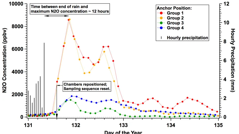
individual data points for N2O concentration. ... 50 Figure 10. Net concentration of N2O in headspace of simple flow-through chambers (groups

1 - 4) and hourly precipitation amounts for the period May 11, 2015 (DOY 131) to May 15, 2015 (DOY 135). Dashed line added to aid visual identification of trend between individual data points for N2O concentration. ... 51 Figure 11. Illustration of linear interpolation between individual non-steady state static

chamber measurements. Period of elevated N2O emissions as suggested by

measurements of N2O concentrations using the simple flow-through chambers added to facilitate visual interpretation of data. Period: May 6 (DOY 126) to May 18 (DOY 138), 2015... 53 Figure 12. Illustration of linear interpolation between individual non-steady state static

chamber measurements with an added data point reflecting an estimate of the start of elevated N2O emissions (DOY 135.5). Period of elevated N2O emissions as suggested by measurements of N2O concentrations using the simple flow-through chambers added to facilitate visual interpretation of data. Period: May 6 (DOY 126) to May 18 (DOY 138), 2015. ... 54 Figure 13. The natural log of the N2O concentration from the simple flow-through chambers

versus time since the peak N2O concentration and a function of group sampling position. Period: DOY 131.849 to DOY 136.432. ... 57 Figure 14. Comparison between estimated N2O flux using an exponential decay function

(12)

Figure 15. Cumulative N2O flux derived from three different approaches: linear interpolation; linear interpolation with adjustment for start of the increase in N2O emissions; and linear interpolation with adjustment for start of the increase in N2O emissions combined with an exponential decay curve to describe the peak in N2O emissions. The error bars are one standard deviation for n = 4 sampling positions. ... 59 Figure 16. Water-filled pore space (WFPS) and precipitation from April 24 to September 23,

2015 (DOY 114 to 246). WFPS increased following precipitation and quickly decreased. The only instance where the 60% WFPS threshold for N2O emissions occurred for more than 10 minutes was on May 11, 2015 (DOY 131) from 6:10 to 7:10 AM. ... 62 Figure B 1. Standard curve for static-chamber flux measurements made between 7 June and

29 July 2014. At the top of the figure is the residual standard deviation (RSD) showing how close the observed values are to the expected concentration values. ... 76 Figure B 2. Standard curve for static-chamber flux measurements made between 29 July and

31 October 2014. At the top of the figure is the residual standard deviation (RSD) showing how close the observed values are to the expected concentration values. ... 76 Figure B 3. Standard curve for measurements made between 20 April and 3 September 2015. At the top of the figure is the residual standard deviation (RSD) showing how close the observed values are to the expected concentration values. ... 77 Figure C 1. Average N2O concentration in glass vials sealed with red septa over time

Average vials and red rubber septa versus time. Vials (n=10) were filled with 2000 ppbv N2O on day 0, and the N2O concentration was measured for three consecutive days following filling. ... 80 Figure C 2. Nitrous oxide concentrations in glass vials sealed with red rubber septa over time as a percent of 2000 ppbv N2O. Vials (n=10) were filled with 2000 ppbv N2O on day 0, and the N2O concentration was measured for three consecutive days following filling. 81 Figure D 1. Average N2O concentrations by glass vials sealed with red rubber septa over

time. Vials (n=10) were filled with 2000 ppbv N2O and one dissected red rubber septum on day 0, and the N2O concentration was measured for three consecutive days following filling. ... 84 Figure D 2. Average N2O concentrations in glass vials sealed with red rubber septa over time

as a percent of 2000 ppbv N2O. Vials (n=10) were filled with 2000 ppbv N2O and one dissected red rubber septum on day 0, and the N2O concentration was measured for three consecutive days following filling. ... 85 Figure E 1. Static chamber measurements were made 18.63, 42.63, 66.63 and 90.63 hours

after the peak flux. Shown here are the peak flux values (A values) calculated using derived decay curve (Eq. 2) as a percent of the A value calculated using the static

chamber measurements made 18.63 hours after the peak. ... 88 Figure I 1. Schematic layout of the chamber groups and trailer in Field 6 at CEFS in

(13)

(14)

CHAPTER 1

Throughout Earth’s 4.5 billion-year history, average global temperatures have

fluctuated. For at least the last 500,000 years the earth has experienced periods of warming

and cooling, called interglacial and glacial periods, respectively, which occur cyclically

(American Association for the Advancement of Science, 2009; Fletcher, 2013).

Approximately every 100,000 years the glacial period is interrupted by a prolonged

interglacial period that lasts approximately 15,000 to 20,000 years. Approximately 10,000

years ago the earth entered an interglacial period called the Holocene epoch, which ushered

in the rise of agriculture. While the natural processes of climate change continued,

agriculture introduced new anthropogenic effects on the atmosphere and the climate that

continue into the present day.

Global warming, or an increase in the average global temperature, is a natural part of

an interglacial period. The main driver of global warming is radiative forcing, or an imposed

change in the balance between the energy earth receives from the sun and the energy that

radiates back into space (IPCC, 2007). Global warming creates changes in average long-term

weather patterns over various regions, which is climate change. Prior to 1750 AD, radiative

forcing occurred mainly as a result of natural causes (IPCC, 2007). Since pre-industrial times

(1750 AD), anthropogenic causes have increased radiative forcing by approximately 2.3

W/m2 (IPCC, 2014). From 1880 to 2012 the average land and ocean surface temperature

increased approximately 0.85 °C (IPCC, 2014).

Evidence overwhelmingly suggests that the cause of global warming is anthropogenic

(15)

America, agree that the earth’s temperature increase is mainly the result of an increase in

anthropogenic greenhouse gas emissions since 1750 AD (American Association for the

Advancement of Science, 2009).

Greenhouse Gases

The major natural and anthropogenic greenhouse gases are water vapor (H2O), carbon

dioxide (CO2), methane (CH4), nitrous oxide (N2O), ozone (O3), and chlorofluorocarbons

(CFCs) (USEPA, 2013). Water vapor, clouds and CO2 account for 95% of the total

greenhouse effect (Schmidt et al., 2010).

The greatest source of anthropogenic radiative forcing is CO2. The atmospheric

residence of CO2 is 10s to 1000s of years, and it is being released into the atmosphere at a

greater rate than any other greenhouse gas (Schmidt et al., 2010; Fletcher, 2013). However,

CH4 and N2O are also important greenhouse gases, having approximately 28 and 300 times,

respectively, the global warming potential of CO2 over a 100-year period (USEPA, 2013;

IPCC, 2014).

Land use change and the burning of fossil fuels are the greatest anthropogenic sources

of greenhouse gas emissions worldwide (IPCC, 2007; Fletcher, 2013). Deforestation,

industrial processes, agriculture, and anaerobic microbial respiration of organic matter in

landfills are also important sources of emissions.

Opportunities for mitigation of greenhouse gases are present in many industries.

Increasing the use of renewable energy sources such as solar and wind power in industrial

(16)

to mitigating anthropogenically induced global warming. Agriculture also presents

opportunities for mitigation of multiple greenhouse gases, including N2O.

Nitrous Oxide

N2O is a greenhouse gas with an atmospheric lifetime of 114 years (IPCC, 2007) and

roughly 300 times the global warming potential of CO2 over a 100-year period (USEPA,

2013). Chemical transformations of N2O in the stratosphere lead to production of NO and

NO2, which are ozone depleting gases (IPCC, 2007; Ravishankara et al., 2009). Based on

direct observations and model predictions, the atmospheric concentration of N2O in 2005 was

estimated to be 319 ± 0.12 ppb, which is well above the estimated pre-industrial range of

180-260 ppb (IPCC, 2007). Since 1750 AD, N2O atmospheric concentrations have risen

~18% (IPCC, 2007; USEPA, 2013), and the current rate of N2O increase in the atmosphere is

0.25% yr-1 (IPCC, 2007). It is estimated that 4.1-8.1% of the anthropogenic greenhouse effect

can be attributed to N2O (Mosier et al., 1998; IPCC, 2007).

The primary natural and anthropogenic sources of N2O release into the atmosphere

include the manufacturing of nylon; burning of plant-derived materials; atmospheric

oxidation of ammonia; emissions from river, estuarine and ocean ecosystems; and the

microbial processes of nitrification (NTR), denitrification (DNF) and nitrifier denitrification

in soil ecosystems (Bateman and Baggs, 2005; IPCC, 2007). The greatest amount of N2O

(17)

Agricultural Nitrous Oxide Emissions

Nitrification and Denitrification

Aerobic NTR and anaerobic DNF in agricultural soils are the most significant

anthropogenic sources of N2O (IPCC, 2007; Reay et al., 2012), with cropland soils

accounting for 64% of direct annual anthropogenic release of N2O into the atmosphere

(USEPA, 2013). NTR is the aerobic microbial transformation of ammonium into nitrogen

(N) oxides (NO3- and NO2-) (Thangarajan et al., 2013). DNF is an anaerobic stepwise process

during which microbes respire N-oxides to nitric oxide (NO), N2O and dinitrogen gas (N2)

(Philippot et al., 2007; Felber et al., 2012; Senbayram et al., 2012).

DNF requires limited O2 availability, NO3- and NO2-, electron donors from organic

carbon (C) compounds, and microorganisms capable of DNF (Philippot et al., 2007).

Anaerobic conditions are most often induced by precipitation or irrigation events filling the

soil pore space with water. Fertilizers, NTR and soil organic matter provide a supply of NO3

-and NO2-, and in the case of organic fertilizers, a source of organic C.

Natural factors that influence soil N2O emission rates include soil texture, pore

structure and aeration, NO3-_{and NO2}- _{availability, soluble C, pH, moisture, and temperature}

(Avrahami et al., 2002; Philippot et al., 2007; Baggs et al., 2010). Wetting-drying events and

freeze-thaw cycles also influence production and emissions of N2O from soils (Sehy et al.,

2003; Dilly et al., 2011).

Management Effects on Emissions

The main management-related factors that affect N2O emissions are tillage and

(18)

effects on soil N2O emissions are not clearly articulated in the literature. Grandy et al. (2006)

found no significant difference in N2O emissions between conventional-till (CT) and no-till

(NT) systems over six years of corn production in southwestern Michigan. Smith et al.

(2012) found no difference in cumulative N2O flux from CT and NT fields growing corn in

northeast Alabama. In a 3-year study in Nashville, TN, average cumulative N2O emissions

were higher in CT than in NT (0.48 and 0.29 mg m-2 h-1, respectively) (Deng et al., 2015).

Venterea et al. (2011) found no difference in area-scaled N2O emissions between CT and NT

during three corn growing seasons in Minnesota. However, when N2O was expressed per unit

yield of grain, emissions were 52% greater in NT than in CT.

Type of N applied can affect the physical and chemical properties of the soil

(Mulvaney et al., 1997), thus influencing the potential for DNF to occur. Timing of N

application to synchronize with crop uptake can reduce N2O emissions, due to there being

less N substrate available for DNF (Millar et al., 2010). Cardenas et al. (2010) observed a

linear increase in cumulative emissions with N application rates up to 150 kg ha-1, after

which cumulative emissions increased exponentially with N rate.

Modeling Nitrous Oxide Emissions

Models are necessary for extrapolating measured N2O emissions data across larger

spatial and temporal scales. They allow for estimates of N2O emissions when direct

measurement is not an option. Models can also predict potential impacts of management on

greenhouse gas emissions. The most often used models for estimating N2O emissions from

soils are the DeNitrification DeComposition model (DNDC), the DayCent model, and the

(19)

DeNitrification DeComposition Model

The DNDC model is a process-based model that simulates C and N cycling and

accounts for environmental and management parameters in estimating and simulating N2O

emissions (Gilhespy et al., 2014; Uzoma et al., 2015). The original DNDC model started as a

way to simulate N2O emissions from agricultural soils in the US. It has been modified over

the past two decades to work with many ecosystems, including wetlands and forests. The

DNDC model can help pinpoint where the bulk of emissions are occurring in a region,

allowing for strategic, directed mitigation.

In the DNDC model ecological drivers of trace gas emissions are linked to soil

environmental variables, which are then linked to trace gas production through nitrification,

denitrification and fermentation. The three main driving factors of N2O production or

consumption in the DNDC model are soil redox potential (Eh), dissolved organic C (DOC)

concentration, and labile N concentration (Giltrap et al., 2010). DNDC can predict both

nitrification and denitrification at the same time using the ‘anaerobic balloon’ concept

(Giltrap et al., 2010; Gilhespy et al., 2014).The anaerobic balloon consists of anaerobic

microsites that expand or shrink based on the redox potential of the soil.

While they did not compare cumulative N2O emissions between the DNDC estimates

and static chamber measurements, Deng et al. (2016) observed that the DNDC model was

able to accurately predict both the timing and magnitude of temporal variations in N2O

emissions over three cropping seasons in Nashville, TN. In a study comparing DNDC N2O

estimates to continuous measurement data in a poorly drained Dystric Vertisol soil, Uzoma et

(20)

This is in part likely due to the inability of the DNDC hydrology framework to account for

water flow during periods of high rainfall. The DNDC model continues to be modified for

worldwide applications.

DayCent Model

DayCent is a process-based model used to estimate N2O emissions in the annual

Environmental Protection Agency (EPA) report to the United Nations Framework

Convention on Climate Change (UNFCCC). DayCent is similar to DNDC in that it uses

submodels controlled by nutrient inputs, management activities, and climate conditions to

simulate greenhouse emissions (Scheer et al., 2014).

In a two-year study growing wheat and cotton in Australia, DayCent accurately

predicted the timing and magnitude of emissions from fertilizer additions to cotton (Scheer et

al., 2014). DAYCENT predictions of cumulative N2O emissions were within 16% of

measured values from Kentucky bluegrass and ryegrass lawns in Colorado (Zhang et al.,

2013). DayCent predictions compared to measured data in an Irish sandy clay loam pasture

suggested that applied N remaining in the soil horizon was sufficient to generate a second

peak in N2O emissions in late summer, however no such peak was observed (Abdalla et al.,

2010). Except for this overestimate, the model-generated cumulative flux only deviated by

1% from the measured flux. In this same study, DayCent provided a better fit than DNDC for

(21)

Emission Factor Model

The emission factor model is used by the Intergovernmental Panel on Climate Change

(IPCC) to estimate countrywide N2O emissions. Evidence suggests that N application rate is

the most important factor for predicting N2O emissions when comparing N source,

application method, rate and timing. Numerous studies agree that N2O cumulative emissions

linearly increase with N rate, giving rise to the emission factor model used in the IPCC Tier 1

approach (Millar et al., 2010). The IPCC has set a default Tier 1 soil N2O emission factor of

1%, meaning that 1% of inorganic N made available in soils by human activity is lost as

N2O.

In an analysis examining the quality of data used to develop the default IPCC soil

N2O emission factor, Rochette and Eriksen-Hamel (2008) found very low confidence levels

in 50% of N2O flux reports. They also found that while the reported data might be useful for

comparisons between treatments within a study, the experimental bias limited comparison of

fluxes between studies. The IPCC default 1% emission factor is not always in agreement

with measured emission factors. In a 2-year, static-chamber method study Cardenas et al.

(2010) observed that N2O emissions increased exponentially, rather than linearly, with N

rate, giving rise to emission factor values both lower and higher than 1%.

Measuring Nitrous Oxide Emissions from Soils

Calculating cumulative N2O flux from an agro-ecosystem involves measuring N2O

emissions from the soil several times during a study period, interpolating between flux

measurements and then integrating under the curve to generate the cumulative flux value. No

(22)

established as the official standard because methods cannot be calibrated in an absolute

manner. The two main categories of methods used for measuring soil N2O flux are the

chamber and micrometeorological techniques. Each has its advantages and disadvantages,

and the use of either method depends on the objectives of the study.

Micrometeorological Techniques

With micrometeorological techniques, fluxes are measured from a large footprint

without disturbing the soil ecosystem using tower-based instrumentation (Uzoma et al.,

2015). These techniques are ideal for measuring and integrating trace gas flux over areas of

0.01-1.0 km2 (Laville et al., 1999). They do not work as well for smaller source areas or for

assessing flux over a relatively short distances, such as plot-based designs that are typical in

agricultural studies. The main sources of error in measuring N2O flux with

micrometeorological techniques are due to the high spatial and temporal variability of N2O

soil emissions (Nicolini et al., 2013). Micrometeorological techniques are also the most

expensive method for measuring N2O flux.

Comparisons of micrometeorological and chamber-based N2O flux measurements

present both agreement and disagreement between measured values (Nicolini et al., 2013),

with greater agreement occurring when the flux sources were well represented by both

methods. Micrometeorological techniques are difficult to replicate, which gives preference to

using chambers to quantify N2O flux measurements in replicated, plot-based field

(23)

Chamber Techniques

Chamber-based techniques for measuring flux at the soil-to-atmosphere interface

include non-flow-through (static) chambers and flow-through (dynamic or continuous)

chambers. Regardless of chamber type, the chamber footprint area is typically less than 1 m2.

Static chamber-based flux methodology is the least expensive option and the most

commonly used method for measuring soil N2O emissions (Parkin and Venterea, 2010). This

method relies on diffusion transport of N2O from the soil pores to the headspace inside the

chamber. In the static chamber approach, a chamber anchor is inserted into the soil, and an

airtight chamber lid with a septum is placed on the anchor. During chamber closure, gas is

extracted multiple times and stored in syringes or pre-evacuated glass vials for lab analysis

on a gas chromatograph (GC). Individual static-chamber fluxes are measured by calculating

the rate of change of trace gas concentration during chamber deployment time over the area

that the chamber covers. Then cumulative flux is estimated by interpolating between

individual flux measurements over time and integrating under the curve.

Continuous chambers are similar to static chambers in that they include an anchor

inserted into the soil and a chamber lid placed over the anchor during chamber deployment.

In continuous chambers air is constantly flowing through the chamber headspace, and the

flux is calculated based on mass balance by taking the difference in N2O concentrations at

the inlet and the outlet over time. Inlet and outlet N2O concentrations are often determined

using on-site instrumentation such as an infrared gas analyzer housed in a trailer. With

(24)

method: by interpolating between individual flux measurements and integrating under the

curve for a total cumulative flux value.

For both static and continuous chamber techniques, chamber lids can be placed on the

anchors either manually or using an automated system. While manual chamber closure is the

least expensive and most widely used option, automatic chamber closure in conjunction with

a continuous system provides greater temporal resolution of soil N2O emissions (Parkin,

2008), while potentially reducing environmental artifacts created by keeping a chamber lid in

place for long periods of time. Measuring N2O flux using automated chamber closure has

been accomplished through three main means: using a cover that slides into place over the

anchor (Ambus and Robertson, 1998), using a lid that swings up and rests at a 90° angle in

standby mode (Breuer et al., 2000; Denmead et al., 2010), and through using a rotary arm

that moves the chamber lid onto or off of the anchor (Fassbinder et al., 2013). The use of

automated chamber enclosures requires a reliable power source using a permanent power

line, a generator, or a simple solar-power system on site.

Static Chamber Flux Calculation Methods

Before cumulative flux can be estimated, flux from individual static chamber

measurements must be calculated. The method of calculating flux collected from a single

static chamber measurement introduces a large source of possible uncertainty, and there is no

single recommended best flux calculation method. Selection of a flux calculation method is

based on several factors including number and spacing of measurements in time, auxiliary

(25)

provides a method for minimizing both bias and variance (Eq. 1) (de Klein and Harvey,

2015):

MSE = Variance + Bias2 ₍₁₎

Often a combination of flux calculation methods will provide the least error for a

given dataset. In addition to linear regression, there are 5 main methods of flux calculation

(de Klein and Harvey, 2015): Hutchinson and Mosier (HM), quadratic regression (QR),

non-steady state diffusive flux estimator (NDFE), the modified Hutchinson and Mosier method

(HMR), and the chamber bias correction method (CBC). Each method calculates flux from

one set of static chamber measurements at a time.

When used with curvilinear data, linear regression tends to underestimate flux.

However, it is historically one of the most widely used flux calculation methods because of

its simplicity and ease of use. The HM method (Hutchinson and Mosier, 1981) requires

exactly three equally timed measurements, and it is not recommended because of

improvements upon the method that reduce imprecision. The HMR method (Pedersen et al.,

2010) is a modification of the HM method, with the added consideration for lateral gas

transport beneath the chambers. It requires 4 or more sampling points, and is available as an

R software package that calculates flux with both the HMR and linear regression methods.

The HMR software also provides an estimate of the MSE and allows users to manually select

linear regression or HMR as the best fit for each set of chamber measurements. The QR

method (Wagner et al., 1997) requires at least 3 sampling time points, with no restriction on

the spacing of the measurements. It is less biased than linear regression for

(26)

methods. The NDFE method (Livingston et al., 2006) is recommended for 4 or more time

points. It provides an estimate of flux at time 0, yet it is not recommended for use with large

data sets. Further, it can give unexpectedly high flux values and possibly deliver more than

one flux value for the same data set when calculated multiple times. The CBC method

(Venterea, 2010) first determines flux using a linear regression, HM, or QR, which is then

multiplied by a correction factor. It requires soil bulk density, temperature, clay content and

water content data, and can be used with 3 or 4 sampling time points.

Cumulative Flux Calculation

Regardless of whether a micrometeorological, static chamber or flow-through

chamber technique is used to measure flux from the soil to atmosphere interface, cumulative

flux is most often estimated using the trapezoid, or linear, method of interpolating between

individual flux measurements and then integrating under the curve. Both over and

underestimation of cumulative flux can occur, depending on how aligned or misaligned

individual flux measurements are with capturing peak flux events.

Few studies that assess addressing N2O temporal variability in a static-chamber

sampling protocol exist. Parkin (2008) used an automated, continuous system to measure

N2O flux every 6 hours for 8 months to obtain a “true” cumulative N2O flux estimate. He

then subsampled the data to evaluate how static-chamber sampling frequency affected the

cumulative N2O estimates. When sampling at 14-day intervals, cumulative emissions

estimates were between -43 and 64% of the “true” cumulative estimate. A cumulative flux

estimate within ±10% of the “true” value was obtained by measuring flux every 3 days. The

(27)

recommends implementing a sampling protocol that addresses the temporal variation of the

N2O source based on when emissions peaks are expected (de Klein and Harvey, 2015).

Standardization of the Static Chamber Method

While no standard method exists for measuring N2O from soils, the static chamber

method with manual chamber lid placement is the de facto standard because of its ease of use

and low cost. It is a very common method, and there are as many ways to implement it as

there are researchers using it. While the method allows comparisons between treatments

within a study, the differences between how researchers implement the static chamber

method inhibit cross-study comparisons of results due to biases. Therefore the USDA

Agricultural Research Service (ARS) has attempted to standardize the static chamber method

protocols in a project called GRACEnet. The GRACEnet protocol aims to facilitate the

widespread adoption of a common methodology to aid in site inter-comparisons (Parkin and

Venterea, 2010). The protocol is being utilized across the United States and is a best guess

effort to optimize sensitivity, limit bias and variance, and allow accurate interpolation and

extrapolation over space and time, despite the inability to precisely assess the extent of bias

associated with any given design. As the protocol is relatively new, the effectiveness of the

GRACEnet protocol in aiding site inter-comparisons has yet to be determined.

The NOCMG (de Klein and Harvey, 2015) is a collaboration between international

N2O researchers that aims to standardize the methods for measuring agricultural N2O

emissions using chamber techniques and improve inter-comparability between findings of

international studies. The document details recommendations for the key aspects of chamber

(28)

requirements and evolving standards for each of the key aspects. The key aspects that the

NOCMG covers include chamber design, deployment, air sample collection, storage and

sample analysis, data analysis and data reporting. Despite their efforts, the NOCMG authors

faced difficulty in reducing uncertainty in cumulative emissions estimates due to spatial and

temporal variability.

Spatial and Temporal Variability

The GRACEnet protocol and the NOCMG take into account several variables that

can affect N2O flux measurements including soil disturbance, perturbations in temperature,

pressure and humidity, gas mixing, chamber placement, frequency and timing of

measurements, spatial variation, and method of flux calculation. However, despite these

efforts to optimize and standardize the static chamber technique, minimizing bias due to

spatial and temporal variability remains a difficulty. This is due to the labor-intensive

demands of the technique coupled with the fact that spatial and temporal patterns N2O

emissions are not fixed like a defined soil property.

Spatial variability of emissions is extremely high and has the potential to introduce

uncertainty in flux estimates (Chadwick et al., 2014). Reported relative standard deviations

(RSD) of spatial variability from static-chamber based measurements ranges from 18% to

397% (Smith and Dobbie, 2001). In a study using static chambers to measure N2O flux over

15,360 m2_{of grazed and mowed grasslands, Velthof et al. (1996) estimated that 375 to 1240}

chambers were needed to measure flux within 10% of the true mean. GRACEnet and

NOCMG recommend sampling a minimum of 2 and 3 chambers per plot, respectively, to

(29)

The temporal pattern of N2O flux is driven by soil C and N dynamics, and it is

heavily influenced by factors that occur cyclically, such as diurnal and seasonal temperature

fluctuations, as well as by factors that occur irregularly, such as rainfall and N application (de

Klein and Harvey, 2015). Accounting for temporal variability when measuring N2O flux

from soils reduces uncertainty and provides data that is useful for improving models. This

allows greater precision in estimating N2O flux over areas of all sizes, and assists in

developing plans for targeted mitigation in areas and at times with the greatest flux. Since

characterizing the temporal pattern of N2O emissions with the static chamber method is

logistically unrealistic, researchers predict when peak flux events are most likely to occur and

then focus on sampling heavily around those times. Wetting events create anaerobic

conditions in soils that stimulate N2O production. Thus to account for precipitation-induced

emissions, static-chamber sampling typically occurs once between 12 to 72 hours after the

end of a wetting event. To account for management-induced N2O emissions, sampling

frequency will often be increased following a management event until emissions return to

baseline levels. During times when peak emissions are not expected, sampling will typically

occur on an arbitrary schedule, such as once per month, or not at all.

Peak N2O flux can both climax and decay within a matter of hours following a

precipitation or management event (Stehfest and Bouwman, 2006; Fassbinder et al., 2013).

Unless flux is measured continuously, the timing and magnitude of the N2O emissions are

unknown (Smith and Dobbie, 2001; Parkin, 2008). Despite increased manual sampling

frequency, the potential for failing to capture both the peak and decay of a flux remains.

(30)

lead to overestimation of cumulative emissions (de Klein and Harvey, 2015). Further, failure

to measure flux during an unexpected peak flux event can introduce bias in cumulative N2O

flux estimates (Smith and Dobbie, 2001; Parkin, 2008; Parkin and Venterea, 2010; de Klein

and Harvey, 2015).

Objective

Without knowing the pattern and magnitude of N2O emissions over time,

uncertainties due to temporal variability remain, thus contributing to uncertainty in

estimating cumulative emissions (Smith and Dobbie, 2001; Parkin, 2008; Reeves and Wang,

2015). Our objective was to reduce uncertainty in cumulative N2O flux estimates due to

temporal variability. We created a continuous flow-through chamber system to monitor the

temporal emissions curve and provide an index of the pattern and magnitude of N2O

emissions throughout the growing season. Static chamber measurements were used to

quantify N2O flux based on recommendations from both the GRACEnet and NOCMG

protocols. The continuous index was used as a guide for adjusting cumulative emissions

estimates from static-chamber measurements by identifying both the occurrence and the

beginning of flux events, timing and relative magnitude of the peak, and decay of flux

following the peak. The continuous flow-through system was deployed during in a no-till

conventional field at the Center for Environmental Farming Systems (CEFS) in Goldsboro,

(31)

References

Abdalla, M., Jones, M., Yeluripati, J., Smith, P., Burke, J., Williams, M., 2010. Testing DayCent and DNDC model simulations of N2O fluxes and assessing the impacts of climate change on the gas flux and biomass production from a humid pasture. Atmospheric Environment 44, 2961–2970.

Ambus, P., Robertson, G.P., 1998. Automated Near-Continuous Measurement of Carbon Dioxide and Nitrous Oxide Fluxes from Soil. Soil Science Society of America Journal 62, 394.

American Association for the Advancement of Science, 2009. Climate Change Statement. Avrahami, S., Conrad, R., Braker, G., 2002. Effect of Soil Ammonium Concentration on

N2O Release and on the Community Structure of Ammonia Oxidizers and Denitrifiers. Applied and Environmental Microbiology 68, 5685–5692.

Baggs, E.M., Smales, C.L., Bateman, E.J., 2010. Changing pH shifts the microbial source as well as the magnitude of N2O emission from soil. Biology and Fertility of Soils 46, 793–805.

Bateman, E.J., Baggs, E.M., 2005. Contributions of nitrification and denitrification to N2O emissions from soils at different water-filled pore space. Biology and Fertility of Soils 41, 379–388.

Breuer, L., Papen, H., Butterbach-Bahl, K., 2000. N2O emission from tropical forest soils of Australia. Journal of Geophysical Research 105, 26353.

Cardenas, L.M., Thorman, R., Ashlee, N., Butler, M., Chadwick, D., Chambers, B., Cuttle, S., Donovan, N., Kingston, H., Lane, S., Dhanoa, M.S., Scholefield, D., 2010.

Quantifying annual N2O emission fluxes from grazed grassland under a range of

inorganic fertiliser nitrogen inputs. Agriculture, Ecosystems and Environment 136, 218– 226.

Chadwick, D.R., Cardenas, L., Misselbrook, T.H., Smith, K. a., Rees, R.M., Watson, C.J., McGeough, K.L., Williams, J.R., Cloy, J.M., Thorman, R.E., Dhanoa, M.S., 2014. Optimizing chamber methods for measuring nitrous oxide emissions from plot-based agricultural experiments. European Journal of Soil Science 65, 295–307.

de Klein, C., Harvey, M., 2015. Nitrous Oxide Chamber Methodology Guidelines. Ministry for Primary Industries, Wellington, New Zealand.

Deng, Q., Hui, D., Wang, J., Iwuozo, S., Yu, C.-L., Jima, T., Smart, D., Reddy, C., Dennis, S., 2015. Corn Yield and Soil Nitrous Oxide Emission under Different Fertilizer and Soil Management: A Three-Year Field Experiment in Middle Tennessee. Plos One 10. Deng, Q., Hui, D., Wang, J., Yu, C., Li, C., Reddy, K.C., Dennis, S., 2016. Assessing the

(32)

349.

Denmead, O.T., Macdonald, B.C.T., Bryant, G., Naylor, T., Wilson, S., Griffith, D.W.T., Wang, W.J., Salter, B., White, I., Moody, P.W., 2010. Emissions of methane and nitrous oxide from Australian sugarcane soils. Agricultural and Forest Meteorology 150, 748– 756.

Dilly, O., Pfeiffer, E.-M., Yanai, Y., Hirota, T., Iwata, Y., Nemoto, M., Nagata, O., Koga, N., 2011. Accumulation of nitrous oxide and depletion of oxygen in seasonally frozen soils in northern Japan – Snow cover manipulation experiments. Soil Biology and

Biochemistry 43, 1779–1786.

Fassbinder, J.J., Schultz, N.M., Baker, J.M., Griffis, T.J., 2013. Automated, low-power chamber system for measuring nitrous oxide emissions. Journal of Environmental Quality 42, 606–14.

Felber, R., Conen, F., Flechard, C.R., Neftel, a., 2012. Theoretical and practical limitations of the acetylene inhibition technique to determine total denitrification losses.

Biogeosciences 9, 4125–4138.

Fletcher, C., 2013. Climate Change: What The Science Tells Us. Wiley, Hoboken. Gilhespy, S.L., Anthony, S., Cardenas, L., Chadwick, D., Li, C., Misselbrook, T., Rees,

R.M., Salas, W., Sanz-cobena, A., Smith, P., Tilston, E.L., Topp, C.F.E., Vetter, S., Yeluripati, J.B., 2014. First 20 years of DNDC (DeNitrification DeComposition): Model evolution. Ecological Modelling 292, 51–62.

Giltrap, D.L., Li, C., Saggar, S., 2010. DNDC: A process-based model of greenhouse gas fluxes from agricultural soils. Agriculture, Ecosystems and Environment 136, 292–300. Grandy, A.S., Loecke, T.D., Parr, S., Robertson, G.P., 2006. Long-term trends in nitrous

oxide emissions, soil nitrogen, and crop yields of till and no-till cropping systems. Journal of Environmental Quality 35, 1487–1495.

Hirsch, A.I., Michalak, A.M., Bruhwiler, L.M., Peters, W., Dlugokencky, E.J., Tans, P.P., 2006. Inverse modeling estimates of the global nitrous oxide surface flux from 1998-2001. Global Biogeochemical Cycles 20.

Hutchinson, G., Mosier, A., 1981. Improved soil cover method for field measurement of nitrous oxide fluxes. Soil Science Society of America Journal 45, 311–316.

IPCC, 2007. Climate Change 2007: The Physical Science Basis. Contribution of Working Group I to the Fourth Assessment Report of the Intergovernmental Panel on Climate Change. Cambridge University Press, Cambridge, United Kingdom and New York, NY, USA.

(33)

Laville, P., Jambert, C., Cellier, P., Delmas, R., 1999. Nitrous oxide fluxes from a fertilised maize crop using micrometeorological and chamber methods. Agricultural and Forest Meteorology 96, 19–38.

Livingston, G.P., Hutchinson, G.L., Spartalian, K., 2006. Trace Gas Emission in Chambers. Soil Science Society of America Journal 70, 1459.

Millar, N., Robertson, G.P., Grace, P.R., Gehl, R.J., Hoben, J.P., 2010. Nitrogen fertilizer management for nitrous oxide (N2O) mitigation in intensive corn (Maize) production: An emissions reduction protocol for US Midwest agriculture. Mitigation and Adaptation Strategies for Global Change 57, 185–204.

Mosier, A., Kroeze, C., Nevison, C., Oenema, O., Seitzinger, S., van Cleemput, O., 1998. Closing the global N2O budget: nitrous oxide emissions through the agricultural nitrogen cycle. Nutrient Cycling in Agroecosystems 52, 225–248.

Mulvaney, R.L., Khan, S.A., Mulvaney, C.S., 1997. Nitrogen fertilizers promote denitrification. Biology and Fertility of Soils 24, 211–220.

Nicolini, G., Castaldi, S., Fratini, G., Valentini, R., 2013. A literature overview of micrometeorological CH4 and N2O flux measurements in terrestrial ecosystems. Atmospheric Environment 81, 311–319.

Parkin, T.B., 2008. Effect of sampling frequency on estimates of cumulative nitrous oxide emissions. Journal of Environmental Quality 37, 1390–5.

Parkin, T.B., Venterea, R.T., 2010. Chamber-Based Trace Gas Flux Measurements, in: Follett, R.. (Ed.), Sampling Protocols. pp. 3–1 to 3–39.

Pedersen, A.R., Petersen, S.O., Schelde, K., 2010. A comprehensive approach to soil-atmosphere trace-gas flux estimation with static chambers. European Journal of Soil Science 61, 888–902.

Philippot, L., Hallin, S., Schloter, M., 2007. Ecology of Denitrifying Prokaryotes in Agricultural Soil, in: Advances In Agronomy. Elsevier Inc., pp. 249–305.

Ravishankara, A.R., Daniel, J.S., Portmann, R.W., 2009. Nitrous oxide (N2O): the dominant ozone-depleting substance emitted in the 21st century. Science 326, 123–5.

Reay, D.S., Davidson, E. a., Smith, K. a., Smith, P., Melillo, J.M., Dentener, F., Crutzen, P.J., 2012. Global agriculture and nitrous oxide emissions. Nature Climate Change 2, 410–416.

Reeves, S., Wang, W., 2015. Optimum sampling time and frequency for measuring N2O emissions from a rain-fed cereal cropping system. Science of The Total Environment 530-531, 219–226.

(34)

Scheer, C., Del Grosso, S.J., Parton, W.J., Rowlings, D.W., Grace, P.R., 2014. Modeling nitrous oxide emissions from irrigated agriculture: Testing DayCent with high-frequency measurements. Ecological Applications 24, 528–538.

Schmidt, G., Ruedy, R., Miller, R.L., Lacis, A., 2010. Attribution of the present-day total greenhouse effect. Journal of Geophysical Research 115.

Sehy, U., Ruser, R., Munch, J.C., 2003. Nitrous oxide fluxes from maize fields: Relationship to yield, site-specific fertilization, and soil conditions. Agriculture, Ecosystems and Environment 99, 97–111.

Senbayram, M., Chen, R., Budai, A., Bakken, L., Dittert, K., 2012. N2O emission and the N2O/(N2O+N2) product ratio of denitrification as controlled by available carbon substrates and nitrate concentrations. Agriculture, Ecosystems and Environment 147, 4– 12.

Smith, K. a., Dobbie, K., 2001. The impact of sampling frequency and sampling times on chamber-based measurements of N2O emissions from fertilized soils. Global Change Biology 7, 933–945.

Smith, K., Watts, D., Way, T., Torbert, H., Prior, S., 2012. Impact of Tillage and Fertilizer Application Method on Gas Emissions in a Corn Cropping System. Pedosphere 22, 604–615.

Stehfest, E., Bouwman, L., 2006. N2O and NO emission from agricultural fields and soils under natural vegetation: summarizing available measurement data and modeling of global annual emissions. Nutrient Cycling in Agroecosystems 74, 207–228.

Thangarajan, R., Bolan, N.S., Tian, G., Naidu, R., Kunhikrishnan, A., 2013. Role of organic amendment application on greenhouse gas emission from soil. The Science of the Total Environment 465, 72–96.

USEPA, 2013. Inventory of U.S. Greenhouse Gas Emissions and Sinks: 1990-2011. Washington, DC.

Uzoma, K.C., Smith, W., Grant, B., Desjardins, R.L., Gao, X., Hanis, K., Tenuta, M., Goglio, P., Li, C., 2015. Assessing the effects of agricultural management on nitrous oxide emissions using flux measurements and the DNDC model. Agriculture, Ecosystems & Environment 206, 71–83.

Velthof, G.L., Jarvis, S.C., Stein, a., Allen, a. G., Oenema, O., 1996. Spatial variability of nitrous oxide fluxes in mown and grazed grasslands on a poorly drained clay soil. Soil Biology and Biochemistry 28, 1215–1225.

Venterea, R.T., 2010. Simplified Method for Quantifying Theoretical Underestimation of Chamber-Based Trace Gas Fluxes. Journal of Environmental Quality 39, 126–135. Venterea, R.T., Bijesh, M., Dolan, M.S., 2011. Fertilizer source and tillage effects on

(35)

Quality 40, 1521–31.

Wagner, S.W., Reicosky, D.C., Alessi, R.S., 1997. Regression models for calculating gas fluxes measured with a closed chamber. Agronomy Journal 89, 279–284.

Zhang, Y., Qian, Y., Bremer, D.J., Kaye, J.P., 2013. Simulation of Nitrous Oxide Emissions and Estimation of Global Warming Potential in Turfgrass Systems Using the

(36)

CHAPTER 2

Introduction

Nitrous oxide (N2O) is a trace gas with approximately 298 times the global warming

potential as carbon dioxide (USEPA, 2013). Globally N2O accounts for about 5% of the total

greenhouse effect (Philippot et al., 2007). Compared to pre-industrial levels, atmospheric

concentrations of N2O have risen about 19% (IPCC, 2007). Nitrous oxide emissions from

agricultural soils account for approximately 64% of the total annual anthropogenic U.S. N2O

emissions (USEPA, 2013).

While there is no standard method of measuring soil N2O emissions, the vented,

non-steady state static chamber method is the most widely employed (Parkin and Venterea,

2010). In the static chamber method an anchor is inserted into the soil, and a gas-tight

chamber lid with a septum is placed over the anchor for a short period of time. At regular

intervals during chamber closure, air samples are extracted from the chamber headspace and

injected into gas-tight containers for laboratory analysis (de Klein and Harvey, 2015). This

method is relatively inexpensive, easy to transport and use, and works well in smaller

plot-size agricultural experiments.

The static chamber method is limited in its ability to address the spatial and temporal

variability (Chadwick et al., 2014) of N2O flux. Flux is the rate of gas exchange between the

soil-to-atmosphere interface per area per time. Without a standardized protocol,

method-induced bias makes it very difficult to compare N2O flux data across studies (Rochette and

Eriksen-Hamel, 2008). The rate of change of gas in the chamber headspace is not a fixed

(37)

causing flux measurements to be biased low, depending on the flux calculation methods used

(Parkin and Venterea, 2010). The GRACEnet protocol (Parkin and Venterea, 2010) offers

suggestions to optimize sensitivity, limit bias and variance, and allow accurate interpolation

and extrapolation over space and time using the static chamber method. However,

GRACEnet’s protocols are only a best guess, due to the inability to precisely assess the

extent of bias associated with any given design (Parkin and Venterea, 2010).

The method of calculating flux for an event introduces a large source of possible

uncertainty. Methods for calculating flux range from simple linear regression to complex

methods that require auxiliary data inputs and a specific number of sample points evenly

spaced in time. There is no single recommended best method for flux calculation. Selection

of a flux calculation method that will best minimize uncertainty is based on several factors

including number and spacing of measurements in time, auxiliary data available, and the

calculated mean square error (MSE) for a given technique. The MSE provides a method for

minimizing both bias and variance (Eq. 1) (de Klein and Harvey, 2015):

MSE = Variance + Bias2 ₍₁₎

Often a combination of flux calculation methods will provide the least error for a

given dataset. In addition to linear regression, there are 5 main methods of flux calculation

(de Klein and Harvey, 2015): Hutchinson and Mosier (HM), quadratic regression (QR),

non-steady state diffusive flux estimator (NDFE), the modified Hutchinson and Mosier method

(HMR), and the chamber bias correction method (CBC). Each method calculates flux for one

static chamber at a time. When used with curvilinear data, linear regression tends to

(38)

methods because of its simplicity and ease of use. The HM method (Hutchinson and Mosier,

1981) requires exactly three equally timed measurements, and it is not recommended because

of improvements upon the method that reduce imprecision. The QR method (Wagner et al.,

1997) requires at least 3 sampling time points, with no restriction on the spacing of the

measurements. It is less biased than linear regression for convex-downward curvature, yet it

is more biased in regards to this curvature than other non-linear methods. The NDFE method

(Livingston et al., 2006) is recommended for 4 or more time points. It provides an estimate of

flux at time 0, yet it is not recommended for use with large data sets. Further, it can give

unexpectedly high flux values and also possibly deliver more than one flux value for the

same data set when calculated multiple times. The HMR method (Pedersen et al., 2010) is a

modification of the HM method, with the added consideration for lateral gas transport

beneath the chambers. It requires 4 or more sampling points, and is available as an R

software package that calculates flux with both the HMR and linear regression methods. The

HMR software also provides an estimate of the MSE and allows users to manually select

linear regression or HMR as the best fit for each flux value. The CBC method (Venterea,

2010) first determines flux using a linear regression, HM, or QR, which is then multiplied by

a correction factor. It requires soil bulk density, temperature, clay content and water content

data, and can be used with 3 or 4 sampling time points.

Spatial variability of emissions can exhibit relative standard deviations greater than

100% (Smith and Dobbie, 2001; Parkin, 2008; Parkin and Venterea, 2010). In a study using

static chambers to measure N2O flux over 15,360 m2 of grazed grassland, (Velthof et al.,

(39)

to be within 10% of the true mean. A minimum of three chamber replicates per treatment are

recommended to reduce spatial variability (de Klein and Harvey, 2015). Consideration of

variation in the topography and differences in the field conditions due to management

activities should be accounted for when determining criteria for chamber placement.

Chambers with a larger footprint can also reduce spatial variability (Parkin and Venterea,

2010). When hotspots are identifiable, such as by visible signs of urine patches (Oenema et

al., 1997), a sampling design can be developed to reduce spatial variability due to such

hotspots. Increased resolution in the temporal characterization of soil N2O flux is necessary

for assessing and addressing uncertainty due to spatial variation.

Small- and large-scale temporal variations of N2O emissions can impact cumulative

estimates of emissions. Day-to-day magnitudes of emissions can differ substantially

(Halvorson and Del Grosso, 2012; Reeves and Wang, 2015), further complicating the ability

to estimate cumulative N2O emissions from static-chamber based data. Fassbinder et al.

(2013) observed that weekly static chamber sampling missed peak N2O fluxes that were

recorded by a continuous monitoring system, leading to underestimation of cumulative flux

using static chamber data. Identifying key time points when N2O flux is expected and

developing a sampling strategy to capture the flux temporal pattern can potentially address

temporal variability when using the static chamber method to estimate cumulative flux.

Denitrification is an anaerobic microbial process that produces N2O (Galloway,

2003). Wetting events create anaerobic conditions in soils that trigger denitrification.

Therefore N2O sampling typically occurs once between 12 to 72 hours after a wetting event

(40)

the pattern and magnitude of each temporal emissions curve is unknown, thus leading to

possible uncertainties in estimating cumulative emissions (Smith and Dobbie, 2001; Parkin,

2008; Reeves and Wang, 2015). Temporal variability is reduced by more frequent flux

measurements (Smith and Dobbie, 2001; Parkin, 2008).

Our objective was to reduce uncertainty in cumulative N2O flux estimates due to

temporal variability. We attempted to use a relatively simple continuous monitoring system

to create an index of the temporal N2O emissions curve, while relying on non-steady state

static chamber measurements for quantitative flux measurements. The temporal emissions

curve was used to address uncertainties in the static-chamber based estimation of cumulative

flux due to temporal variation. While systems for continuously and quantitatively measuring

N2O flux are available, they add cost and complexity, especially for assessing flux in more

than 1 or 2 locations. Our system mirrors that created by Fassbinder et al. (2013), with the

key difference being that we did not use the continuous system quantitatively, but rather

qualitatively to inform static-chamber sampling protocols and the manipulation of results

from static-chamber measurements in estimating cumulative emissions.

Materials and Methods

Study Site Location

The research site was situated in the Farming Systems Research Unit (FSRU) at the

Center for Environmental Farming Systems (CEFS) near Goldsboro, NC (35°23′N, 78°02′W,

elevation 35 m above sea level). The FSRU is an 81-hectare interdisciplinary long-term study

of five systems laid out in a randomized complete block design with three replicates. The

(41)

temperature of 16.7˚C and precipitation of ~1240 mm yr-1 (Arguez et al., 2010). The Neuse

River borders CEFS on three sides, creating high spatial variability in soil types within the

river basin.

Actual measurements were taken in a subplot of the Best Management Practices

(BMP) treatment of the Conventional Cash Cropping System. The BMP has a three-year

rotation of corn, soybean and grain sorghum, with winter cover crops used in all three years.

The BMP is split into subplots of conventional tillage and no-till. Measurements were

restricted to a no-till subplot of the BMP, to allow chamber anchors to remain undisturbed as

much as possible, with a corn-soybean rotation that started in spring 2013 and winter cover

crops.

Because of the high spatial variability in soil types across the FSRU, the area has

been mapped for defined diagnostic soil units via an intensive GPS-based soil survey. The

diagnostic, dominant soil in the no-till subplot used in this study is a well-drained Wickham

sandy loam (fine-loamy, mixed, semiactive, thermic Typic Hapludult). Average depth to the

water table is greater than 200 cm (Soil Survey Staff et al., 2015). Selected soil physical and

chemical properties of the 0-30 cm soil depth for the study site are: pH 6.1; bulk density 1.53

g cm-3; 19% clay; 61.7% sand; and 19.4% silt (Soil Survey Staff et al., 2015) (Bell and

(42)

(43)

(44)

Temperature, Rainfall, and Soil Moisture/Temperature - 2015 Growing Season Hourly average precipitation and air temperature data were obtained from the NC

Climate Retrieval and Observations Network of the Southeast Database (CRONOS:

http://climate.ncsu.edu; Dec. 12, 2015). The actual recording instrumentation is part of the

NC Environment and Climate Observing Network (NC ECONet: Latitude: 35.37935˚,

Longitude: -78.0448˚, Station ID: GOLD – Cherry Research Station). The ECONet station is

located approximately 0.83 km from the no-till BMP subplot monitored in this project. Soil

moisture and water content within the BMP subplot were measured every 10 minutes using

an EM50® Data Logger and 5TM® sensors (Decagon Devices, Inc.) inserted at a depth of

7.62 cm below the soil surface. Monthly descriptive summaries for each of these parameters

are provided in Table 1 for the period April 24, 2015 to September 3, 2015.

Table 1.Total precipitation and descriptive summaries of daily air temperature recorded by NC ECONet Station GOLD-Cherry Research Station, and 10-minute readings of soil temperature and moisture content (depth: 7.62 cm) within the no-till BMP subplot monitored in this project.

Period: Date (DOY)

24 April (114)-31 May (151)

1 June (152)-30 June (181)

1 July (182)-31 July (212)

1 Aug (213)-3 Sept. (246) Precipitation (mm)

Total 96.27 70.10 101.09 116.33

Ambient Air Temperature (˚C)

Mean 19.7 26.3 26.7 25.1

Std. Dev. 6.2 5.0 4.1 4.3

Minimum 3.4 13.6 16.7 14.2

Maximum 31.6 37.8 36.3 37.1

Soil Moisture Content (m3_/m-3₎

Mean 0.162 0.078 0.074 0.115

Std. Dev. 0.027 0.020 0.034 0.039

Minimum 0.167 0.041 0.034 0.038

Maximum 0.258 0.124 0.237 0.292

Soil Temperature (˚C)

Mean 20.9 28.5 28.5 27.3

Std. Dev. 4.1 3.0 2.4 2.6

Minimum 14.7 21.7 23.2 21.7

(45)

No-Till Corn

The study site subplot consists of 8 rows that are 102-m long within one rep of the

no-till BMP block. A 2-row buffer was designated on either side of the subplot. Corn (Zea

mays var. KDC 64-69, treated and Roundup® ready) was planted in the study site subplot of

the BMP no-till system at a rate of 28,000 seeds ac-1 spaced 17.8 - 19.1 cm apart on April 24,

2015 (DOY 114). Liquid UAN was applied on April 27, 2015 (DOY 117) at a rate of 70 lbs

N ac-1 and again on May 29, 2015 (DOY 149) at a rate of 87 lbs N ac-1. Immediately after

planting, pre-herbicide Bicep II Magnum (S-metolachlor + Atrazine) was applied at a rate of

2.1 qt. ac-1. Immediately following sidedress N application, glysophate (Roundup) and

atrazine were applied at a rate of 1 qt. ac-1 each.

Nitrous Oxide Measurements

Non-Steady State Vented Static Chambers – Field Measurements

The soil-atmosphere exchange of N2O was measured at least once a week and for 3-4

consecutive days after rain events. Samples were collected midmorning of each sampling

day, from April 30, 2015 (DOY 120) to September 2, 2015 (DOY 245), for a total of 30

measurement dates.

A vented, non-steady state closed-chamber technique was used (Hutchinson and

Livingston, 2001). Twenty-four PVC (16 in-row, 8 between-row) anchors (20.32 cm

diameter x 20.32 cm height) were inserted to a depth of 17.78 cm. The anchors were placed

in 4 groups (6 anchors per group) along the length of the no-till BMP subplot (Appendix I).