Exact and Inexact Methods for Solving the Problem
Of View Selection for Aggregate Queries
Zohreh ASGHARZADEH TALEBI1, Rada CHIRKOVA2, and Yahya FATHI1
1 Operations Research Program, NC State University, Raleigh, NC 27695,
{zasghar,fathi! ! !}@ncsu.edu
2 Computer Science Department, NC State University, Raleigh, NC 27695, [email protected]†
Abstract. We present a study of the followingwarehouse view-selection problem: Given a frequency distribution on parameterized aggregate queries on a data warehouse, return definitions of aggregate views that, when materialized in the warehouse, would reduce the evaluation costs of the frequent queries. Optimizing the layout of stored data using view selection has a direct impact on the performance of data warehouses. However, the optimization problem is intractable, even under natural restrictions on the types of queries of interest. We introduce an integer-programming model to obtain optimal solutions for the warehouse view-selection problem, and propose a heuristic to obtain competitive inexact solutions where our exact method is inapplicable. We show that both our approaches can be used to solve realistic-size instances of the problem. In addition, we experimentally compare our methods to those of Harinarayan et al. (1996) and Shukla et al. (1998), and delineate applicability areas for these and our approaches.
Keywords:business intelligence, data reporting, OLAP, business intelligence cycle, schema specification selection, view selection, data warehouse design, data analysis tools.
1
Introduction
As data warehouses keep growing in size, evaluating many common queries — such as aggre-gate queries — in OLAP may require significant transformations of large volumes of stored data. Aggregate queries are widely used in data warehouses and decision support. Optimiza-tion based on the reuse of query answers is particularly promising for aggregate queries, as often an enormous amount of data is scanned to produce a single aggregate value. As a result, the requirement of good overall performance of frequent and important business intelligence queries necessitates optimal choices in choosing and executing query plans. A significant aspect of query performance is the choice of auxiliary data (e.g., indexes) used in query answering. In modern commercial database systems, a common type of auxiliary data is materialized views — relations that were computed by answering certain queries on the (original) stored data in the database and that can be used to provide, without time-consuming runtime transformations, “precompiled” information that is relevant to the user query. We give an example of using materialized views to answer select-project-join queries with aggregation in a star-schema (see Kimball et al. (2002)) data warehouse.
! ! ! This author’s work is partially supported by the National Science Foundation under Grant No. 0321635.
Example 1. Consider a data warehouse with three stored relations:Sales(CID,
DateID,Qty-Sold,Discount),Customer(CID,CustName,Address,City,State), andTime(DateID,Day,
Month,Year). Here, Sales is the fact table, andCustomer and Time are dimension tables.
Let the query workload have two queries, Q1 and Q2. Q1 asks for the total quantity of products sold per customer in the last quarter of the year 2006. Q2 asks for the maximal product quantity sold per year for all years after 2000 to customers in North Carolina.
Q1: SELECT c.CID, SUM(QtySold) Q2: SELECT t.Year, MAX(QtySold) FROM Sales s, Time t, Customer c FROM Sales s, Time t, Customer c
WHERE s.DateID = t.DateID AND s.CID = c.CID WHERE s.DateID = t.DateID AND s.CID = c.CID AND Year = 2006 AND Month >= 10 AND Month <= 12 AND Year > 2000 AND State = ‘NC’
GROUP BY c.CID; GROUP BY t.Year;
We can use techniques from Harinarayan et al. (1996) to show that the following view V can be used to give exact answers to each of Q1 and Q2.
V: SELECT s.CID, Year, Month, State, SUM(QtySold) AS SumQS, MAX(QtySold) AS MaxQS FROM Sales s, Time t, Customer c
WHERE s.DateID = t.DateID AND s.CID = c.CID GROUP BY s.CID, Year, Month, State;
Evaluating the queries Q1 and Q2 using the view V is likely to be more efficient than using their original definitions, as using V allows the DBMS to avoid taking expensive joins of the stored tables and may also save some time in grouping and aggregation. !
We consider the following warehouse view-selection problem: Given a frequency distribu-tion on parameterized aggregate queries on a star-schema data warehouse, and given a set of constraints (e.g., a storage limit on the amount of disk space that can be used to store materialized views), return definitions of views that, when materialized, would satisfy the constraints and reduce the evaluation costs of the frequent queries. As design of materialized views is an important component of query processing in data warehouses (see Baralis et al. (1997), Harinarayan et al. (1996), Kalnis et al. (2002), Shukla et al. (1998), Theodoratos et al. (1997), and Yang et al. (1997)) and of automated query-performance tuning (see IBM and Microsoft; Shasha et al. (2002)), the problems of selecting views and of answering queries using views have been studied thoroughly in the literature.
Generally, spending more time on designing views tends to pay off, as greater improve-ment can thereby be achieved in the query performance. As the number of beneficial views tends to be prohibitive even for simple query workloads (Agrawal et al. (2000); Chirkova et al. (2002); Harinarayan et al. (1996)), it is not practical to use exhaustive enumeration to obtain derived data that would globally minimize query costs. Several approaches (see, e.g., Agrawal et al. (2000); Gupta et al. (1997); Harinarayan et al. (1996); Shukla et al. (1998)) have been proposed to efficiently design good-quality sets of derived data for SQL queries. We continue the work of Gupta et al. (1997) and Harinarayan et al. (1996) of study-ing view-selection algorithms that are competitive, that is, provide optimality guarantees on their outputs without necessarily exploring the entire search space of views. We present a formal model of warehouse view selection, explore competitive techniques for designing and using views in this context, experimentally compare our techniques to previous approaches of Harinarayan et al. (1996) and Shukla et al. (1998), and delineate applicability areas for all of the methods involved.
1. We model warehouse view selection as an integer-programming (IP) problem and give references to similar IP structures in the literature. Our exact method for solving the view-selection problem uses our IP model and returns optimal solutions. In addition, we propose an heuristic that reduces, in the input to the IP model, the size of the search space of useful views, and provides an inexact methodfor solving the problem.
2. With our IP model and heuristic, we use standard IP-solver software to solve optimally or near-optimally realistic-size instances of the problem on the popular TPC-H benchmark (described in TPC-H) and on real data in the Sloan Digital Sky Survey (SDSS) dataset (described in Szalay et al. (2002)).
3. We study the applicability of our exact and inexact methods for two versions of the view-selection problem, determined by whether the table for the view resulting from joining all the base relations (we call this view raw-data view) is part of the solution.
4. We experimentally compare our two methods with the heuristic approaches of Hari-narayan et al. (1996) and Shukla et al. (1998) and delineate the applicability areas of each approach.
In our experiments we solved hundreds of problem instances, both on TPC-H data (described in TPC-H) and on the SDSS dataset (described in Szalay et al. (2002)). The problem instances used both randomly generated query workloads and queries related by the ancestor-descendant relationship in the sense of the structure used by Harinarayan et al. (1996).
After outlining related work, in Section 2 we provide the background and formal def-initions. Section 3 introduces our IP model of the view-selection problem. We report our experimental results and theoretical analysis in Section 4 (for our IP model) and in Section 5 (for the heuristic we propose in the same section). We report our comparative experiments and our comparison conclusions in Section 6.
Related Work
Designing and using derived data to improve query performance has long been studied in data-intensive systems. A wealth of theoretical results (see Halevy (2001) for a survey) and some practical solutions by Agrawal et al. (2001), Chaudhuri et al. (1995), and Chaudhuri et al. (1998) have been accumulated on using views and indexes in query answering. Answer-ing aggregate queries usAnswer-ing views was considered in relation to data warehouses and data cubes by Agarwal et al. (1996), Chaudhuri and Dayal (1997), Gray et al. (1997), and Widom (1995); results on answering each query using a single view were presented by Gupta et al. (1995), and Srivastava et al. (1996). Recent work of Afrati and Chirkova (2005) and Cohen et al. (1999) considered rewriting aggregate queries using multiple views.
(2001) introduced an end-to-end approach and a system architecture for designing and using materialized views and indexes to answer queries.
In this paper we study the problem of selecting views for aggregate queries on star-schema data warehouses. The setting and assumptions we use generalize those by Gupta et al. (1997), Harinarayan et al. (1996), Kalnis et al. (2002), and Shukla et al. (1998) (in contrast to those by Yang et al. (1997)) — that is, we seek to minimize the total execution costs of the frequent queries under a storage-limit constraint. At the same time, one novelty of our work is in obtaining efficiently optimal or near-optimal solutions for problem instances of realistic sizes, for two versions of the view-selection problem. In the first version, we assume similarly to the approach by Harinarayan et al. (1996) that the raw-data view is always part of the solution set of materialized views. We lift this restriction in the second version of view selection; the resulting problem arises in practice in settings where it is too expensive to maintain efficiently the result of joining all base tables, including data-integration settings where certain views are materialized in the mediator to improve query-processing efficiency (see Halevy (2001)). Our extensive experimental evaluation of the proposed methods allows us to delineate applicability areas for our approaches to view selection, as well as for the methods by Harinarayan et al. (1996), Kalnis et al. (2002), and Shukla et al. (1998).
2
Preliminaries and Problem Specification
We consider relational select-project-join queries with grouping and aggregation (SPJGA queries), posed on star-schema data warehouses ( Chaudhuri and Dayal (1997); Kimball et al. (2002)). Similarly to Gupta et al. (1997); Harinarayan et al. (1996); Kalnis et al. (2002); Shukla et al. (1998), we assume application settings where users frequently ask a limited number of parameterized SPJGA queries, such as itemized daily/weekly/monthly sales reports for a variety of parameters for products, locations, etc. Thus, we assume pa-rameterizedqueries, by allowing arbitrary constant values (i.e., placeholders instead of fixed constants) in the WHERE clauses of the queries, and assume that specific values of these constants are not known in advance.
We consider star-schema data warehouses with a single fact table and a small fixed number of dimension tables, under the following realistic assumptions. First, in each base table all rows have a single fixed (upper bound on) length. Second, the fact table has many more (in fact, magnitudes more) rows than each dimension table. Finally, we assume that each base table has a single index, on the table’s key.
We consider the following warehouse view-selection problem: Given a star-schema data warehouse and for a given frequency distribution on parameterized SPJGA queries, our goal is to minimize the evaluation costs of the queries, by selecting and precomputing views that can be used in answering the queries. We consider this minimization problem under a storage-space limit, which is an upper bound on the amount of disk space that can be allocated for the views. Thus, our problem inputs are of the formI = (D,Q, b), where D is a database, Qis a workload of parameterized queries, with a frequency/importance valuefj for each query j in Q, and b is the (positive integer) value of the storage limit.
We use the following definitions of solutions and of the optimal viewset problem (OV P):
Definition 1. For a problem inputI = (D,Q, b), a set of views V is an admissible viewset
if (1) each query in Q can be rewritten using V, and (2) V satisfies the storage limit b.
Definition 2. For a problem input I = (D,Q, b), an optimal viewset is a set of views V defined on D, such that (1) V is an admissible viewset for I, and (2) V minimizes the cost of evaluating Q on the database DV, among all admissible viewsets for I. Here, DV is the database that results from adding to D the relations for all the views in V computed on D.
Definition 3. (Problem OV P) For a given problem input I = (D,Q, b), find an optimal viewset. A solution for a given instance of OV P consists of a set of materialized views V (which includes the raw-data view onDand all additional views that we choose to materialize) and an association between each element of Q and its corresponding element of V.
We also consider a variation OV P! of the optimal-viewset problem: Unlike OV P, in
OV P! we do not require that the raw-data view be materialized as part of the solution. In Section 4 we present an experimental comparison of two versions of our proposed approach, one for OV P and the other for OV P!.
For the class of SPJGA queries that we consider, our search space of views is the view latticeintroduced by Harinarayan et al. (1996) and adopted in a number of research projects, including those by Kalnis et al. (2002) and Shukla et al. (1998). We now discuss and justify our choice of the search space of views and our cost model.
The view lattice described in Harinarayan et al. (1996) that we use as our search space includes all star-join views with grouping and aggregation (JGA views) on the base tables, such that each view has aggregation on all the attributes aggregated in the input queries, using all the aggregation functions used in the queries. Such views, illustrated by view V in Example 1, are called “multiaggregate views” (see Afrati and Chirkova (2005)). A SPJGA queryQ can be answered using a JGA viewV if the grouping attributes ofV are a superset of the union of attributes in the GROUP BY clause of Q and of the attributes in the WHERE clause of Q that are compared to constants. By definition, each query Q can be answered using the top view (raw-data view) in the lattice.
Q using only the raw-data view, rather than to the cost of answering Q using the original base relations in the data warehouse. The reason is, under our assumptions these two costs are directly proportional to each other.
We now argue why considering just the views in our JGA view lattices is a reasonable option in finding optimal or near-optimal sets of views to materialize when seeking to min-imize the costs of answering sets of parameterized SPJGA queries under a storage limit. (Whenever we refer to finding optimal solutions of this problem, we consider optimality with respect to our view lattices.) First, it is more efficient to answer any SPJGA query using a single JGA view than using a query plan that involves joins of base relations or views. Second, when the values of the constants of a parameterized query are not known in advance, the only option to minimize the response time of all queries in Q is to materialize a single eligible JGA view. Finally, using multiaggregate JGA views permits us to use a single view to answer queries with different aggregation functions, as illustrated by Example 1.
3
Integer Programming Models for
OV P
and
OV P
!In this section we propose integer programming (IP) models for the optimal-viewset problems
OV P and OV P!, and discuss methodologies for solving thes IP models. Since we use these IP models to obtainglobally optimal solutionsforOV P andOV P!, we refer to this approach as an “exact method” for solving OV P and OV P!.
We use the following notation to represent the input I = (D,Q, b) in our IP model:
ai : Size of the view i, for alli ∈ IV, where IV is the index set for all possible views;
b: storage limit;
cij : evaluation cost of answering query j by using view i, for all i ∈ IV and j ∈ Q.
We letcij = +∞if viewicannot be used to answer queryj; otherwise we havecij =ai·fj, where ai is as defined above and fj is the frequency (or importance) of query j. We further define the following decision variables for the IP model.
xi =
!
1 if view i is materialized
0 otherwise for all i ∈ IV
and
yij =
!
1 if we use view i to answer query j
0 otherwise for all i ∈ IV and j ∈ Q
The optimal-viewset problem OV P can now be stated as the following IP model.
Minimize "i ∈ IV "j ∈ Qcijyij (OV IP)
subject to ""i ∈ IV aixi ≤b (1)
i ∈ IV yij = 1 ∀ j (2)
yij ≤xi ∀ i, j such that cij %= +∞ (3)
x1 = 1 (4)
Constraint (1) limits the size of the materialized views to be no more than the storage space b. Constraint (2) states that each query is answered by exactly one view in the set of views. Constraint (3) guarantees that query j can be answered by view i only if view i
is already materialized. Constraint (4) states that the raw-data view is always materialized. The remaining constraints are simply the binary requirements for xi and yij.
We can also modify this model into an IP model for the problem OV P! (see note after Definition 3 in Section 2) by removing constraint (4). This is equivalent to stating that the raw-data view is not required to be materialized. We refer to this modified model asOV IP!. The structure of this IP model is similar to those for the uncapacitated facility location problem (UFL) and the k-median problem. These two problems are well studied in the literature, and relatively large instances of the corresponding IP models can be solved within reasonable time. Several heuristic approaches for solving these problems have also been reported. See Cornuejols et al. (1984) and Krarup et al. (1983) for the facility location problem and Mulvey et al. (1979) for thek-median problem.
A key difference between this IP model and those for the UFL and k-median problems is the presence of relatively large numbers of variables in this model due to the large size of the index set IV. If we have K attributes in the data base, the corresponding size of the set IV is 2K, which leads to 2K variables of type x
i and |Q|2K variables of type yij. For a lattice with K = 15 attributes this implies 32,708 xi-variables and 32,708|Q| yij-variables. Comparatively, in a typical UFL or k-median problem the size of the corresponding IV set is no more than a few hundreds. As a result, the algorithmic strategies that are proven to be effective for solving those models turn out to be not as effective for solving OV IP. In Sections 4 and 5 we discuss some strategies for reducing the size of the set IV and thereby the size of the corresponding OV IP model.
Note that due to the special structure of this IP model the binary requirement for yij can be replaced by a simple non-negativity restriction without affecting the corresponding optimal solution for this model. See Parker et al. (1988) for a discussion of this subject and its theoretical underpinning. This relaxation has a significant impact on reducing the overall computational effort required to solve the IP model, and we use it throughout this paper and in all our experiments.
4
A Computational Experiment with the IP Model
As discussed in Section 3, solving the proposed IP models OV IP or OV IP! allows us to obtain optimal (exact) solutions to problems OV P or OV P!, respectively. In this section we discuss the results of an experiment that we conducted in order to investigate various computational aspects of the proposed model, and determine the limits on the size of problem instances that we can solve in practice using this approach and with today’s technology. We put our results in perspective in Section 6.
We begin by proposing an approach for reducing the search space of views in our exact method. As mentioned earlier, a key hurdle in solving realistic instances of the IP model
OV IP (or OV IP!) is the relatively large number of variables in the model, in particular the
IV, i.e., 2K. In practice we can reduce the size of IV — and hence the number of variables in the model — without affecting the optimal value ofOV IP (orOV IP!), by removing from this set every view i that cannot be used to answer at least one of the queries in the set Q3 (for obvious reasons no such view can be in the optimal solution of OV IP or OV IP!). We refer to the resulting (reduced) index set as IV!. The reduction in size (i.e., IV! versus
IV) depends on the specific queries in the set Q. For each instance in our experiment we construct the corresponding reduced set IV! and report its size.
To determine the limits of the size of the instances that we can solve in practice using our exact method, we constructed and solved a large collection of instances of the problem. All experiments were run on a machine with a 3GHz Intel P4 processor, 1GB RAM, and a 80GB hard drive running Windows XP SP2, and using the IP solver CPLEX/AMPL 9.0. This software uses a branch-and-bound algorithm for solving the IP model, and solves the corresponding linear programming relaxation models using the simplex algorithm.
In Section 4.1 we discuss the datasets that we used in the experiments. In Section 4.2 we report the execution time for a collection of instances from these datasets, and make some observations. Finally, in Section 4.3 we present the results of further experiments that offer additional insight on the applicability of our proposed exact methods.
4.1 Datasets
We used two datasets in our experiments: (1) a TPC-H database benchmark (TPC-H), and (2) a real dataset which is a modified version of the Sloan Digital Sky Survey (SDSS) dataset (Szalay et al. (2002)). Figure 1 shows the sizes of the stored tables for the TPC-H dataset. Size estimates for the lattice were obtained by running the queries for all views on the TPC-H stored data with scale factor of 0.1 and by extrapolating the answer sizes to the sizes of the data (scale factor of 1) used in the experiments. For the SDSS dataset, whose sizes of the stored tables are shown in Figure 2, the view sizes were measured on the original database. The observations we made in our experiments were consistent across the two datasets; therefore, in reporting our results in this section we only use examples from the TPC-H dataset.
4.2 Execution Time
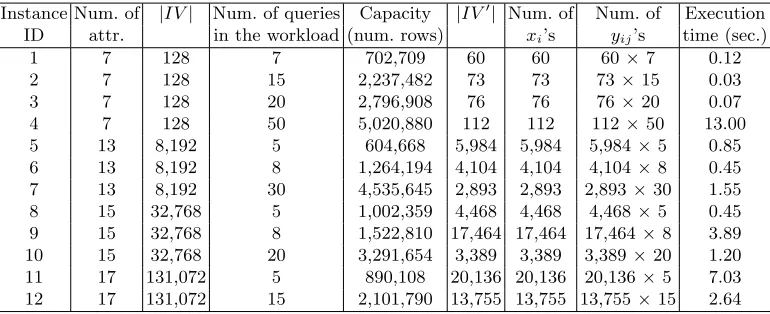
The execution times that we report here pertain to instances from four different TPC-H datasets, i.e., raw-data views with 7, 13, 15, and 17 attributes. (To obtain some raw-data views for the experiments, we used joins of TPC-H tables.) The number of nodes in the view lattices (i.e., the size |IV| of the set IV) for these datasets are 128, 8192, 32768, and 131072, respectively. For each raw-data view we constructed the IP modelOV IP for several instances of the problem, each instance with a different query workloadQ and storage limit
b. We solved each instance using the software package CPLEX/AMPL with a time limit of thirty seconds on the execution time. In Table 1 we give detailed characteristics of twelve
3 In fact, since in our view lattice we havea
i≥ajfor every pair (i, j) such that viewiis an ancestor of viewj, we
Instance Num. of |IV| Num. of queries Capacity |IV!| Num. of Num. of Execution ID attr. in the workload (num. rows) xi’s yij’s time (sec.)
1 7 128 7 702,709 60 60 60×7 0.12
2 7 128 15 2,237,482 73 73 73×15 0.03
3 7 128 20 2,796,908 76 76 76×20 0.07
4 7 128 50 5,020,880 112 112 112×50 13.00
5 13 8,192 5 604,668 5,984 5,984 5,984×5 0.85
6 13 8,192 8 1,264,194 4,104 4,104 4,104×8 0.45
7 13 8,192 30 4,535,645 2,893 2,893 2,893×30 1.55 8 15 32,768 5 1,002,359 4,468 4,468 4,468×5 0.45 9 15 32,768 8 1,522,810 17,464 17,464 17,464×8 3.89 10 15 32,768 20 3,291,654 3,389 3,389 3,389×20 1.20 11 17 131,072 5 890,108 20,136 20,136 20,136×5 7.03 12 17 131,072 15 2,101,790 13,755 13,755 13,755×15 2.64
Table 1.Description of the twelve problem instances in the experiments.
instances of the problem that we could solve within this time limit. Each row of this table corresponds to one instance and gives the number of attributes, the size of the view lattice, the number of queries in the workload Q, and the storage capacity for that instance. For all instances in this experiment we assume that the frequencyfj associated with each queryj in Qis equal to 1. For each instance we also give the size|IV!|of the setIV!, the corresponding number ofxiandyij variables, and the associated execution time that we measured for solving that instance. We make the following observations.
1. Aside from the number of attributes and queries, the size of the IP model (as measured by the number of xi-variables) and its corresponding execution time also depend on the number of view-lattice nodes that are actually included in the model, i.e., on the cardinality of the set IV!. This size is usually larger if some workload queries are placed relatively low in the lattice. Hence, the largest IP model in our experiment does not necessarily pertain to the instance with the largest number of attributes and/or queries. In fact, the largest IP model that we were able to solve within our stated time limit was for instance 11 in Table 1, which is on a 17-attribute lattice with 5 queries. This model has 20,136 xi-variables and 100,680yij-variables, and its execution time is 7.03 seconds. The largest instance of OV P that we were able to solve, however, pertains to instance 12 in Table 1 which is also on the 17-attribute lattice and has 15 queries. The corresponding IP model has 13,755xi-variables and 206,325 yij-variables, and its execution time is only 2.64 seconds (see Asgharzadeh Talebi et al. (2005)). Further, the largest IP model does not necessarily pertain to the longest overall execution time, since the latter also depends on the growth of the search tree in the context of the branch and bound algorithm. In fact, the longest execution time in our experiments pertains to instance 4 in Table 1 with a 7-attribute view lattice and 50 queries. The corresponding IP model has 112xi-variables and 560 yij-variables, and its execution time is 13.00 seconds.
the lower bound obtained for OVIP via its LP relaxation is relatively strong, hence it leads to quick fathoming of most branches in the corresponding branch-and-bound tree. This observation is not uncommon among other IP models with similar structures, such as the UFL problem that we mentioned earlier. In our experiments, every time that CPLEX/AMPL was not able to solve the IP model within our stated time limit, it was also unable to solve its LP relaxation. We report on the quality of this lower bound in detail in Li et al. (2005).
3. The execution time is expected to grow at an exponential rate with the size of the IP model; hence we do not expect it to be practical to solve much larger instances of this IP model using CPLEX/AMPL. At the same time, the instances that we are able to solve are of realistic sizes in practice (cf., e.g., the problem instances used in the experiments in Shukla et al. (1998)), as exemplified in the last few instances in Table 1. This demonstrates that we can use a standard IP solver to obtain verifiably optimal solutions for practical instances of the problem.
4. In our experiments we also studied whether the ancestor-descendant relationships between workload queries influence the runtime or outcome for our approach. In particular, we studied problem instances with “single-path” query workloads, that is, with workloads Q where for each query Q ∈ Q, each remaining query inQ is either a descendant or an ancestor of Q in the view lattice. It is observed in Kotidis et al. (1999) that workload queries with such relationships are likely to occur in query sessions by a single user in data warehouses, where the user performs roll-ups and drill-downs on the data of interest. In our study, we did not observe significant differences in the runtime or outcome for our approach depending on the type of relationships among workload queries. Rather, as mentioned earlier, we observed that the placement of individual queries in the view lattice has a bigger influence on how efficiently the problem instance can be solved by our approach.
4.3 Further Experimental Observations
In addition to observing the execution time for solving the OVIP model as reported above, we also carried out several related experiments with this IP model. In this section we present a summary of our findings.
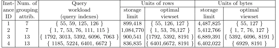
An alternative measure for size requirement: View sizes and query costs are
As units of bytes (instead of rows) is a more realistic measure in the context of view selection, we posit that these units should be employed as the primary units of measurement in problem input. Further details are available in Li et al. (2005).
Inst- Num. of Query Units of rows Units of bytes
ance grouping workload storage optimal storage optimal
ID attrib. (query indexes) limit viewset limit viewset
1 7 {55, 59, 125, 126} 899,418 {55, 126, 127} 4,487,825 {55, 127} 2 7 {1, 7, 53, 76, 111, 115} 1,084,770 {1, 53, 76,127} 5,412,766 {1, 7, 76, 127} 3 13 {1792, 3013, 5392, 6096, 7063} 900,541 {1792, 5392, 8191} 6,889,391 {5392, 6096, 8191} 4 13 {1185, 5224, 6401, 6672} 836,835 {6401,6672, 8191} 6,402,022 {6929, 8191}
Table 2.Solving the OVIP problem for units of rows and bytes.
Solving the OV IP! model:Recall that the only difference betweenOV IP and OV IP!
is that inOV IP! the top raw-data view in the view lattice is not required to be materialized. This version of the problem can arise, for instance, in situations where it may be too expensive to maintain the raw-data view relation, and it is desirable to explore solutions which do not force that relation to be materialized. These situations include data-integration settings where certain views are materialized in the mediator to improve query-processing efficiency (see Halevy (2001)). (Recall that in many cases, the top raw-data view in the view lattices by Harinarayan et al. (1996) is the result of joining several base relations in the star schema.) We carried out a set of experiments in which we constructed and solved several instances of
theOV IP! model and compared the results with those for the correspondingOV IP models.
The details of our experiments are presented in Asgharzadeh Talebi et al. (2005) and Li et al. (2005). In these experiments we observed the following:
– there is no appreciable difference between the computational requirements for solving
OV IP and OV IP!, and
– although in some instances the results obtained via OV IP andOV IP! are identical (i.e.,
OV IP! selects the raw-data view in the optimal set), there are also many instances for
which OV IP! obtains solutions with significantly smaller objective-function values.
5
A Heuristic Procedure for Solving OVIP
In this section we present an inexact (heuristic) method for solving the optimal viewset problem OV IP. The main idea used in this heuristic method is to further prune the search space for candidate views and hence the size of the corresponding IP model, thus allowing larger instances of the problem to be solved in reasonable execution time. Of course when we do so, we can no longer guarantee that the optimal solution for the IP model OV IP (or
OV IP!) is in fact optimal for the corresponding problem OV P (or OV P!).
in fact optimal for the underlying OV P (or OV P!), we need to include all elements of the candidate set IV! in the IP model. But if we do not seek this guarantee of optimality, we can further reduce the size of the set by removing all elements (i.e., nodes of the lattice) that we deem as not-so-promising elements of the set IV! in the IP model. This could lead to significant reduction in the size of the corresponding model OV IP (or OV IP!).
To this end we limit ourselves to a subset ofIV!consisting of views that either correspond to some queries in Qor are ancestors of two or more of these queries. We define a view (or query)v1 to be an ancestor for another view (or query)v2 if the collection of attributes that define v2 is a proper subset of the collection of attributes that define v1; in this context we refer to v2 as the child (or descendant) of v1. We refer to the resulting collection of views
as a restricted viewset IV r. We then construct and solve the corresponding IP model with this restricted viewset, which would likely have fewer variables than the original OV IP (or
OV IP!). We refer to this IP model as OV IP r (or OV IP r!). In Section 5.1 we outline a
procedure by which we construct the restricted viewset IV r and the resulting input matrix for the corresponding IP model, and discuss its computational requirements. In Section 5.2 we report the results of a computational experiment with the corresponding IP model OV IP r.
5.1 Restricted Viewset IV r
Given a datasetD withkattributes and a set of queries QonD, we defineQ! to be a subset of Q consisting of those elements of Q that are not themselves a child or a descendant of another element of Q. We now define a node of the view lattice to be an i-level ancestor of
Q, for i = 2,3, . . . ,|Q!|, if it is an ancestor for i distinct elements of Q! and its size is less that the sum of the sizes of these distinct elements. Using this terminology, we refer to the views associated with elements of the setQ! as the 1-level ancestors ofQ. For allr such that 1≤ r ≤ |Q!|, we define the r-level restricted viewset for Qas the set of all i-level ancestors of the set Q for all i ∈ {1, . . . , r}. This r-level restricted viewset is the set of views in the view lattice that we use to construct the corresponding restricted version OV IP r of the IP model OV IP.
Note that if we letr=|Q!|then the resultingOV IP ris guaranteed to produce an optimal solution for the original problem. At the same time, this IP model could be quite large. We submit that even if we limit the value of r to be much smaller than |Q!|, members of the
At this point we need to be mindful of the additional computational effort required to construct the restricted viewsetIV rand the corresponding IP modelOV IP r. This computa-tional effort is proporcomputa-tional to the maximum number of nodes in the setIV r, i.e.,"ri=1Ci|Q!|, where Ci|Q!|= i!(|Q|Q!!|−|!i)! is the combination “|Q!| choose i”.
In this heuristic procedure, there are two major steps: In the first step we build the restricted viewset IV r consisting of "ri=1Ci|Q!| views. In order to build a view at level i, for 2 ≤ i ≤ r, we need to take the union of the attributes of i distinct queries. The order of complexity of this operation is O(i). Thus, the computational requirement of this step is O("ri=1iCi|Q!|). The second step is to build the input matrix for the corresponding IP model. To do so, for each selected view we need to find out which of the |Q| queries in the query workload can be answered by that view. In the worst case, for each view this will take time O(|Q|k), where k is the number of attributes in the lattice. Thus, the com-putational requirement of this step is O(|Q|k"ri=1Ci|Q!|). Considering the computational requirements of these two steps, the overall computational requirement of the heuristic pro-cedure isO("ri=1iCi|Q!|+|Q|k"ri=1Ci|Q!|), which isO((r+k|Q|)|Q!|r
) or simplyO(|Q|r+1). For low values ofrthis effort is relatively small, but it increases rapidly withr. Note that the computational experiments that we report in Section 5.2 show that we are likely to obtain good results even with low values of r.
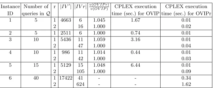
5.2 A Computational Experiment with OV IP r
Our objective in this section is to recommend a reasonable value forr. To do so, we solve five instances optimally using the OV IP model. Then we solve each instance using the OV IP r
model with r = 1. For those instances for which we do not get the optimal solution using
OV IP r with r = 1, we use OV IP r with r = 2. We continue increasing the value of r and
proceed in a similar manner until we get optimal solutions for all instances.
These five instances are constructed in the following manner. All instances are on the 17 attribute TPC-H dataset. In instances 1 and 3, each query in Q has 6, 7, or 8 attributes and in instances 2 and 4, each query inQhas 11, 12, or 13 attributes. In these instance the number of attributes for each query is randomly selected between 6 and 13. We also assume that the frequency associated with each query is equal to one. Furthermore, we select the specific queries in instances 1 and 3 from the lower levels of the lattice, and select queries in instances 2 and 4 from the upper levels of the lattice. The results of our experiments are presented in the first five rows of Table 3.
In this table, for each instance we report the number of queries, sizes of the sets IV! and
IV r, and the ratio of the cost obtained by the heuristic (v(OV IP r)) to the optimal cost
(v(OV IP)). Based on our experimental results, we make the following observations:
1. In one instance (instance ID 2), we find the optimal solution using OV IP r with r = 1. In the remaining four instances (instances 1, 3, 4, and 5), we find the optimal solution using OV IP r with r= 2.
2. For each instance, the size of the setIV r is significantly smaller than the size of the set
IV!. (On average, the ratio |IV!|
Instance Number of r |IV!| |IV r| v(OV IP r)
v(OV IP) CPLEX execution CPLEX execution
ID queries inQ time (sec.) for OVIP time (sec.) for OVIPr
1 5 1 4663 6 1.045 1.67 0.01
2 16 1.000 0.02
2 5 1 2511 6 1.000 0.74 0.01
3 10 1 5436 11 1.059 3.16 0.01
2 47 1.000 0.04
4 10 1 986 11 1.014 0.44 0.01
2 42 1.000 0.03
5 15 1 5129 15 1.048 6.44 0.01
2 105 1.000 0.09
6 40 1 17422 41 - - 0.34
2 624 - - 1.62
Table 3.Instances solved for OVIPr.
3. For each instance, the execution time for solving OV IP r with CPLEX is significantly lower than the execution time for solving OV IP with CPLEX. In these instances, the time for building the set IV r is negligible.
Using our heuristic algorithm, we solved a large instance on the 17 attribute TPC-H dataset with forty queries where the number of attributes in each query is between 6 and 13. We assumed that the frequency associated with each query is equal to one. Due to the large size of the corresponding OV IP model, we were not able to solve this instance optimally within the time limit of fifteen minutes. However, using our heuristic with r = 1 and r = 2, we were able to solve it in 0.34 and 1.62 seconds, respectively. Information about this instance is presented in the last two rows (instance ID 6) of Table 3, and the corresponding values of the solutions obtained via OV IP r with r = 1 and r = 2 for this instance are v(OV IP r)=148,514,000 and v(OV IP r)=144,020,000, respectively. Obviously, we can no longer guarantee that the solution obtained via OV IP r with r= 2 is an optimal solution for the corresponding OV P.
6
Experimental Comparison with Other Heuristic Procedures
We note that the approaches of both Harinarayan et al. (1996) and Shukla et al. (1998) are applied to instances in which every node of the view lattice is in the query set Q with unit frequency. To compare our methods with the results presented in those papers, we first carry out an experiment in which we consider only problem instances of this type. We refer to these instances as Group 1 instances. We solve each instance in this group using each of the three approaches HHRU, SDN, and OV IP. (Note that applying OV IP r to such instances would not add any additional insights, since the restricted viewset IV r would be identical toIV.) These results are presented in Section 6.1. We then run a second experiment in which we allow the query set Q (that is, the queries with nonnegligible frequencies) to be a relatively small subset of the nodes of the view lattice. We refer to these instances as Group 2 instances. Both procedures HHRU and SDN can be easily adjusted to solve these instances. In this case, we solve each instance of the problem using each of the four proceduresHHRU,SDN, OV IP, and OV IP r. The results are presented in Section 6.2.
To carry out this comparative study, we developed an independent computer program for each of HHRU and SDN. Each program is written in C, uses the same data structures and subroutines as our implementations of OV IP and OV IP r, and was run on the same machine that we used for solving the OV IP models, as described in Section 4.
6.1 A Computational Experiment with Group 1 Instances
In this subsection we present experimental results that compare the performance of proce-dures HHRU, SDN, and OV IP, for the case where the input queries are all the nodes in the lattice, and the frequency of each query is equal to one. The experiments in this section are over six data lattices, which are the 5, 6, and 7 attribute TPC-H data lattices and the 5, 6, and 7 attribute SDSS data lattices. For each data lattice, we set the value of storage space to be the size of the top view plusα×(sum of the sizes of all of the views in the lattice except for the top view), and set α = 0.01,0.05,0.1,0.2,0.3,0.4,0.5,0.6,0.7. Thus, for each data lattice we solved nine problem instances.
Figure 3, which presents the results on the TPC-H data lattices, and Figure 4, which shows the results on the SDSS data lattices, compare the quality of the solutions of HHRU
In our experiments we also measured the execution time for each instance. We observed that the execution time of the SDN algorithm is significantly less than those for each of
OV IP and HHRU. Also, in none of the instances did theOV IP execution time exceed the
HHRU execution time.
6.2 A Computational Experiment with Group 2 Instances
In this group of instances we allowed the query set Qto be a relatively small subset of the nodes of the view lattice. We modified the algorithms ofHHRU and SDN to allow for this condition; in addition, we modifiedSDN to guarantee that it return the (top) raw-data view in each solution. The goal of the experiments was to compare our inexact method OV IP r
(with r= 2) with the modifications of algorithms HHRU and SDN.
In the first set of experiments, whose results are presented in Table 4, the first nine instances are on a 7-attribute TPC-H data lattice. In all of these instances, the number of queries in Qis five, and the number of attributes of each query is chosen randomly between one and six. The tenth instance is on a 13-attribute TPC-H data lattice. In this instance, there are ten queries, and the number of attributes of each query is a random number between one and twelve. We assume that the frequency of each query in the set Q equals one. We solved each instance with each of OV IP r (withr= 2), HHRU, andSDN, and report here the ratios of the costs obtained for each heuristic to the optimal cost.
InstanceID 1 2 3 4 5 6 7 8 9 10
v(OV IP r)
v(OV IP) 1.000 1.000 1.000 1.000 1.000 1.000 1.000 1.000 1.000 1.000
v(HHRU)
v(OV IP) 1.053 1.037 1.081 1.000 1.000 1.000 1.039 1.031 1.000 1.059
v(SDN)
v(OV IP) 1.053 1.000 1.000 1.000 1.000 1.047 1.044 1.000 1.000 1.005
Table 4.Instances solved on TPC-H data lattices to compare the heuristic algorithms.
We did similar experiments over a 7-attribute SDSS data lattice. We solved nine instances, each with five queries, where the number of attributes in each query was a random number between 1 and 6. Again, we assumed that the frequency of each query equals one. The results are presented in Table 5.
InstanceID 1 2 3 4 5 6 7 8 9
v(OV IP r)
v(OV IP) 1.000 1.000 1.000 1.000 1.000 1.000 1.000 1.000 1.000
v(HHRU)
v(OV IP) 1.395 1.000 1.671 1.075 1.000 1.000 1.211 1.012 1.624
v(SDN)
v(OV IP) 1.000 1.127 1.422 1.000 1.056 1.278 1.209 1.137 1.423
Table 5.Instances solved on SDSS data lattices to compare the heuristic algorithms.
also observed that on this collection of instances the execution time ofSDN is significantly lower than that for each of HHRU and OV IP r, and that the execution time of OV IP r is significantly lower than that for HHRU.
We also tried to solve a larger instance on the 17 attribute TPC-H lattice with forty queries using both HHRU and SDN. This is the same instance that we reported earlier as instance 6 in Table 3. As mentioned earlier, we were not able to solve this instance optimally (using OV IP) due to its relatively large size, and the corresponding values obtained via
OV IP rwithr= 1 and with r= 2 arev(OV IP r) = 148514000 andv(OV IP r) = 144020000
obtained in 0.34 and 1.62 seconds, respectively. When we tried to solve this instance using
HHRU and SDN, HHRU did not terminate in 15 minutes, and SDN terminated in 0.68 seconds with v(SDN) = 215866080, which is 45% higher than the v obtained via OV IP r
with r= 1 and 50% higher than the v obtained via OV IP r with r= 2.
In our last set of experiments we considered instances where the frequencies associated with queries in the set Qare not all equal to one. Specifically, we used the Zipfian frequency distribution with the skewness parameter equal to one. We solved five such instances over a 15-attribute TPC-H data lattice, where in each instance the number of elements in the setQ was equal to ten and the frequency associated with each query was obtained from the Zipfian distribution. Also, we solved five instances on a 7-attribute SDSS data lattice. The number of queries in the latter instances varied between three and five.
For brevity, we refrain from giving details regarding these instances. Our observations on these experiments can be summarized as follows:
1. In all of the instances, OV IP r (wirh r = 2) found the optimal solution.
2. For all the instances, the size of IV r was significantly smaller than the size of IV!. On average, the ratio ||IV rIV!|| was 106 for the instances on the 15-attribute TPC-H data lattice and 8 for the instances on the 7-attribute SDSS data lattice.
3. For each instance, the execution time for solving OV IP r with CPLEX was significantly lower than the execution time for solving OV IP with CPLEX. In these instances, the time for building the set IV r was negligible. We further observed that this reduction in execution time is more significant for larger instances.
6.3 Applicability Areas for Warehouse View-Selection Methods
methods are compared with each other, while the HHRU solutions are used to normalize the results. While each randomized-search method is significantly faster than HHRU, it appears that the quality of the HHRU solutions is higher than that of each randomized-search method in many of the experiments reported in Kalnis et al. (2002). Based on these results as reported in Kalnis et al. (2002), we conclude that for the goal of solution quality,
HHRU should probably be chosen over the randomized-search methods of Kalnis et al. (2002) wherever HHRU is applicable, i.e., when its execution time is not excessive. At the same time, the approaches of Kalnis et al. (2002) may be a better option for very high-dimensional problem instances, even though they provide no guarantees on solution quality. (We are unable to make conclusions about the solution quality of the approaches of Kalnis et al. (2002), as those have not been experimentally compared with optimal methods, such as our exact method.)
In comparing our exact and inexact methods to the algorithms HHRU and SDN, our conclusions are as follows:
1. Our exact method OV IP/OV IP! is guaranteed to provide optimal solutions:
(a) for both Group 1 and Group 2 problem instances for view-lattice sizes of up to seven dimensions (cf. the experimental results of Shukla et al. (1998) for SDN, which are given for lattices of sizes up to six dimensions only), and
(b) for much larger view-lattice sizes (up to at least 17 dimensions) for Group 2 instances, depending on the number/positioning of the input queries with nonzero frequencies. 2. Based on our experimental results,r= 2 in OV IP r is an appropriate value for the levels
of views in the lattice that we should consider.
3. TheHHRU approach is never preferable to our proposed exact and inexact methods in solution quality or in runtime efficiency.
4. In terms of the quality of solution, whileSDN is comparable toHHRU when the storage-space constraint is “very tight” or “very loose” (see Figures 3 and 4), the quality of the solutions obtained by these algorithms is usually inferior to that for our proposed approaches. Intuitively, SDN picks the views in the order of their sizes. Typically, the views that can answer many queries are of large size and will not be picked by SDN, yet in many cases the size of such views is smaller than the sum of the sizes of the queries that they can answer. Unlike our approaches, SDN does not appear to give good opportunities for such views to be selected.
5. In terms of runtime efficiency, SDN is always the method of choice.
Bibliography
Afrati, F. and Chirkova, R. (2005) ‘Selecting and Using Views to Compute Aggregate Queries’, Proc. ICDT, pp. 383–397.
Afrati, F., Chirkova, R., Gupta, S. and Loftis, C. (2005) ‘Designing and Using Views to Improve Performance of Aggregate Queries’,Proc. 10th Int’l Conf. on Database Systems for Advanced Applications (DASFAA).
Agarwal, S., Agrawal, R., Deshpande, P., Gupta, A., Naughton, J.F., Ramakrishnan, R. and Sarawagi, S. (1996) ‘On the Computation of Multidimensional Aggregates’,Proc. VLDB, pp. 506–521.
Agrawal, S., Chaudhuri, S. and Narasayya, V.R. (2000) ‘Automated Selection of Materialized Views and Indexes in SQL Databases’,Proc. VLDB, pp. 496–505.
Agrawal, S., Chaudhuri, S. and Narasayya, V.R. (2001) ‘Materialized View and Index Selection Tool for Microsoft SQL Server 2000’,Proc. ACM SIGMOD, p. 608.
Asgharzadeh Talebi, Z., Chirkova, R. and Fathi, Y. (2005) ‘Experimental study of an IP model for the view selection problem’, NC State University, technical report number TR-2005-34, Available from http://www4.ncsu.edu/
∼rychirko/Papers/techReport072005.pdf.
Asgharzadeh Talebi, Z., Chirkova, R. and Fathi, Y. (2006) ‘A Study of a Formal Model For View Selection for Aggregate Queries’,NC State University, technical report number TR-2006-2, Available
fromftp://ftp.ncsu.edu/pub/unity/lockers/ftp/csc anon/tech/2006/TR-2006-2.pdf.
Baralis, E., Paraboschi, S. and Teniente, E. (1997) ‘Materialized View Selection in a Multidimensional Database’,
Proc. VLDB, pp. 156–165.
Chaudhuri, S., Krishnamurthy, R., Potamianos, S. and Shim, K. (1995) ‘Optimizing Queries with Materialized Views’,
Proc. ICDE, pp. 190–200.
Chaudhuri, S. and Dayal, U. (1997) ‘An Overview of Data Warehousing and OLAP Technology’,SIGMOD Record, Vol. 26, No. 1, pp. 64–74.
Chaudhuri, S. and Narasayya, V.R. (1997) ‘An Efficient Cost-Driven Index Selection Tool for Microsoft SQL Server’,
Proc. VLDB, pp. 146–155.
Chaudhuri, S. and Narasayya, V.R. (1998) ‘AutoAdmin ’What-if’ Index Analysis Utility’,Proc. ACM SIGMOD, pp. 367–378.
Chirkova, R., Halevy, A.Y. and Suciu, D. (2002) ‘A formal perspective on the view selection problem’,VLDB Journal, Vol. 3, No. 3, pp. 216–237.
Cohen, S., Nutt, W., Serebrenik, A. (1999) ‘Rewriting Aggregate Queries Using Views’,Proc. PODS, pp. 155–166. Cornuejols, G., Nemhauser, G.L. and Wolsey, L.A. (1984) ‘The uncapacitated facility location problem’,Operations
Research and Industrial Engineering, Cornell University, technical report number 605.
Gray, J., Chaudhuri, S., Bosworth, A., Layman, A., Reichart, D. and Venkatrao, M. (1997) ‘Data Cube: A Relational Aggregation Operator Generalizing Group-by, Cross-Tab, and Sub Totals’,Data Mining and Knowledge Discovery, Vol. 1, No. 1, pp. 29–53.
Gupta, A., Harinarayan, V. and Quass, D. (1995) ‘Aggregate-Query Processing in Data Warehousing Environments’,
Proc. VLDB, pp. 358–369.
Gupta, H., Harinarayan, V., Rajaraman, A. and Ullman, J.D.(1997) ‘Index Selection for OLAP’,Proc. ICDE, pp. 208–219.
Halevy, A.Y. (2001) ‘Answering queries using views: A survey’,VLDB Journal, Vol. 10, No. 4, pp. 270–294. Harinarayan, V., Rajaraman, A. and Ullman, J.D.(1996) ‘Implementing data cubes efficiently’,Proc. ACM SIGMOD,
pp. 205–216.
IBM, ‘Autonomic Computing’,http://www.research.ibm.com/autonomic/. ILOG S.A. (2000) ‘CPLEX 7.0 software package’,http://www.ilog.com.
Kalnis, P., Mamoulis, N. and Papadias, D. (2002) ‘View selection using randomized search’,Data Knowledge Engi-neering, Vol. 42, No.1, pp. 89–111.
Kimball, R. and Ross, M. (2002) ‘The Data Warehouse Toolkit (second edition)’,Wiley Computer Publishing. Kotidis, Y. and Roussopoulos, N. (1999) ‘DynaMat: A dynamic view management system for data warehouses’,Proc.
ACM SIGMOD, pp. 371–382.
Krarup, J. and Pruzan, P.M. (1983) ‘The simple plant location problem: Survey and synthesis’, European Journal Operations Research, Vol. 12, pp. 36–81.
Microsoft Research AutoAdmin Project, ‘Self-Tuning and Self-Administering Databases)’,
http://research.microsoft.com/dmx/autoadmin/default.asp.
Mulvey, J.M. and Crowder, H.P. (1979) ‘Cluster Analysis: An Application of Lagrangian Relaxation’,Management Science, Vol. 25, pp. 329–340.
Parker, R. G. and Rardin, R.L. (1988) ‘Discrete Optimization’,Academic Press.
Shasha, D., Bonnet, P. (2002) ‘Database Tuning: Principles, Experiments, and Troubleshooting Techniques’,Morgan Kaufmann.
Shukla, A., Deshpande, P. and Naughton, J.F. (1998) ‘Materialized View Selection for Multidimensional Datasets’,
VLDB’98, Proceedings of 24rd International Conference on Very Large Data Bases, August 24–27, New York City, New York, USA, pp. 488–499.
Srivastava, D., Dar, S., Jagadish, H.V. and Levy, A.Y. (1996) ‘Answering Queries with Aggregation Using Views’,
Proc. VLDB, pp. 318–329.
Szalay, A.S., Gray, J., Thakar, A.R., Kunszt, P.Z., Malik, T., Raddick, J., Stoughton, C. and VandenBerg, J. (2002) ‘The SDSS SkyServer - Public access to the Sloan Digital Sky Server data’, Microsoft Re-search, Microsoft Corporation, technical report number MSR-TR-2001-104, Available fromftp://ftp.research. microsoft.com/pub/tr/tr-2001-104.pdf; also seewww.sdss.org.
Theodoratos, D. and Sellis, T. (1997) ‘Data Warehouse Configuration’,Proc. VLDB, pp. 126–135. TPC-H, ‘TPC Benchmark H (Decision Support)’,http://www.tpc. org/tpch/spec/tpch2.1.0.pdf. Widom, J.(1995) ‘Research problems in data warehousing’,Proc. CIKM, pp. 25–30.
Region Nation2 Nation1 Orders Customer PartSupp Supplier Part Lineitem
396 2,103 2,103 482,877,440 244,883,456 5,830,541 14,188,544 1,193,906 2,147,483,647
Size (bytes) Name
TPC-H Tables
Fig. 1.Sizes of the TPC-H tables.
Neighbors Field Segment Plate PhotoObj SpecObjAll
1,321 919 621 69,035 38,206,539 200,851,705
Size (bytes) Name
SDSS Tables
Fig. 2.Sizes of the SDSS tables.
HHRU
Fig. 3. Comparison of HHRU, SDN, and
OV IPfor TPC-H data lattices (OVIP provides the optimal solutions).
HHRU
Fig. 4. Comparison of HHRU, SDN, and