A Fault Tolerance framework for Kepler-based Distributed Scientific Workflows.

(1)

ABSTRACT

MOUALLEM, PIERRE A. A Fault Tolerance Framework for Kepler-based Distributed Scientific Workflows. (Under the direction of Dr. Mladen A Vouk).

Scientific Workflow Management Systems (S-WFMS), such as Kepler, have proven to be an

important tool in scientific problem solving. They allow scientific experiments to handle

increased concurrent and longitudinal complexity and larger amounts of data. Since

S-WFMS rely on a multitude of technologies and principles, they share the vulnerabilities and

errors of these technologies, and since they hide the underlying components, identifying

those errors becomes a challenge, especially when operating in a tightly coupled

environment.

Fault tolerance and failure recovery in scientific workflows running in S-WFMS is

still a relatively a young topic. The work done in the domain mostly applies classic fault

tolerance mechanisms, such as Alternative Versions and Check-pointing. Often scientific

workflow systems simply rely on the fault tolerance capabilities provided by their third party

subcomponents such as schedulers, Grid resources, or the underlying operating

systems. When failures occur at the underlying layers, a workflow system sees this as failed

steps in the process, often without additional detail. Therefore, the ability of the system to

recover from those failures may be limited.

The approach described in this dissertation aims to provide a light weight end-to-end

framework implementing fault tolerance in situations where Kepler is the workflow engine.

Based on failure patterns that occur in real-life scientific workflow executions, we present

methodologies which inject recovery fragments into fault-prone scientific workflow models

(2)

failures at different layers of a workflow management architecture. We discuss the

framework in the context of the failures observed in two production-level Kepler-based

scientific workflows, specifically XGC and S3D. The framework is divided into three major

components:

(i) A general contingency Kepler actor that provides a recovery block functionality at the

workflow level. This actor extends the concept of Alternative versions (also known as

Recovery Block) by adding a provenance based scoring scheme to the decision making

process.

(ii) An external monitoring module that tracks the underlying workflow components,

monitors the overall health of the workflow execution, and communicates with the

workflow engine and the contingency actor to better address those errors, and

(iii) A checkpointing mechanism which handles loops, stateless and stateful actor. The

mechanism provides “smart resume” capabilities for cases in which an unrecoverable

error occurs.

This framework takes advantage of the provenance data collected by the Kepler-based

workflows to detect failures and help in fault tolerance decision making. The three

components are interconnected via sockets and database calls.

Capabilities and limitations of the framework are assessed using simulations. The

results show that the presented fault tolerance framework is quite cost effective. Framework

operations incur a marginal overhead, dramatically increase the workflow reliability and at

(3)

(4)

A Fault Tolerance Framework for Kepler-based Distributed Scientific Workflows

by

Pierre A Mouallem

A dissertation submitted to the Graduate Faculty of North Carolina State University

in partial fulfillment of the requirements for the degree of

Doctor of Philosophy

Computer Science

Raleigh, North Carolina

2011

APPROVED BY:

_______________________________ ________________________________

Dr. Nagiza Samatova Dr. Yannis Viniotis

________________________________ ________________________________

Dr. Mladen Vouk Dr. Laurie Williams

(5)

ii

DEDICATION

I dedicate this dissertation to my parents and my brother. I could never have done it without

their constant support, encouragement and faith in me. Thank you for everything you have

(6)

iii

BIOGRAPHY

Pierre Mouallem completed his primary education in Lebanon. He received his Bachelor’s

degree in Computer Science from Notre Dame University, Lebanon. He received his

Master’s degree in Computer Science from NC State University in 2005 and joined the PhD

(7)

iv

ACKNOWLEDGMENTS

I express my sincere gratitude towards my advisor, Dr. Mladen Vouk, for his guidance,

relentless support and encouragement. I also would like to thank Dr. Nagiza Samatova, Dr.

Yannis Viniotis and Dr. Laurie Williams for serving on my committee and for their insight

and assistance.

I would also like to thank my colleagues in the Scientific Process Automation group

(SPA) of the DOE Scientific Data Management Center (SDM) and the SDM group for their

support and help throughout the research. Special thanks to Roselyne Barreto, Norbert

Podhorszki and Scott Klasky from ORNL, Ilkay Altintas and Daniel Crawl of SDSC,

Bertram Ludaescher of UC-Davis, Ayla Khan of the University of Utah and last but not least,

Meiyappan Nagappan of NCSU.

This work has been supported in part by the DOE SciDAC grant DE-FC02-07-ER25484 and

(8)

v

TABLE OF CONTENTS

LIST OF TABLES ... vii

LIST OF FIGURES ... viii

LIST OF ABBREVIATIONS ... x

1 Introduction ... 1

1.1 Scientific Workflows and their role in the Scientific Discovery ... 1

1.2 Challenges facing Scientific Workflows ... 3

1.3 Suggested solution and Dissertation outline ... 4

1.4 Publications ... 6

2 Failure Rate Analysis ... 7

2.1 Definition of failure ... 7

2.2 Failure rates in HPC systems ... 8

2.3 Failure rates in scientific workflow management systems... 10

2.4 Failure rates in Kepler based scientific workflows ... 11

2.4.1 Production level workflows use cases: XGC and S3D ... 11

2.4.2 Typical failure scenarios ... 15

2.4.3 Fault classification ... 17

2.4.4 Failure Analysis ... 22

3 Fault Tolerance mechanisms in scientific workflow management systems ... 25

3.1 Overview ... 25

3.2 Checkpointing ... 25

3.3 Fault tolerance based on Retries and Alternative Versions ... 28

3.4 Summary ... 31

4 Kepler provenance framework ... 33

4.1 Description ... 33

4.2 Provenance database ... 37

4.3 Token tracing... 38

5 Forward Recovery ... 41

5.1 Motivation ... 41

5.2 Contributions ... 42

5.3 Architecture ... 43

5.3.1 Overview ... 43

5.3.2 Workflow interface ... 43

5.3.3 Monitoring layer plug-in ... 45

5.4 Error-state handling ... 45

5 Checkpointing ... 49

6.3 Architecture ... 51

6.3.1 Extensions to the provenance framework and workflow scheduler ... 51

6.3.2 Supported execution models ... 52

(9)

vi

6.4 Recovery scenario ... 55

6.5 Limitations ... 59

7 Error-state Handling Layer ... 60

7.3 Architecture details ... 61

7.3.1 Overview ... 61

7.3.2 Monitoring framework ... 61

7.3.3 Provenance based analysis... 66

7.3.4 Interaction with the Forward Recovery mechanism ... 66

7.4 Recovery scenario ... 67

8 Framework Evaluation ... 68

8.1 Assessment environment ... 68

8.2 Reliability evaluation ... 74

9 Conclusion and future work ... 102

References ... 104

Appendix ... 112

(10)

vii

LIST OF TABLES

Table 2.1: Root-cause analysis ... 19

Table 3.1: Scientific Workflow Management Systems F/T Capabilities ... 32

Table 8.1: Runs of instance 1 in which failures occurred (scenario 2) ... 87

(11)

viii

LIST OF FIGURES

Figure 1.1: Illustration of the control plane orchestration of workflows and resources. ... 2

Figure 1.2: SDM framework that support provenance data collection, workflow management through a dashboard, and a Kepler orchestration engine. ... 3

Figure 2.1: Expected growth in failure rate of multicore/multiprocessor systems ... 9

Figure 2.2: XGC Workflow ... 13

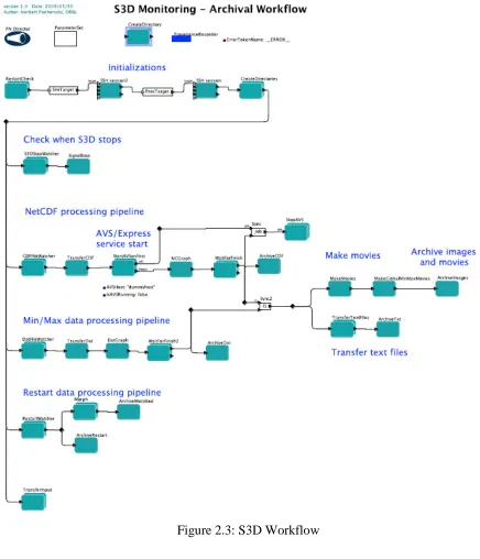
Figure 2.3: S3D Workflow ... 14

Figure 2.4: Failure in Processing Pipeline ... 16

Figure 2.5: Execution Environment Layers ... 20

Figure 2.6: Failure percentage by Layer ... 20

Figure 2.7: Average run time per Computing Resource based on the total run time ... 22

Figure 2.8: Time of failure occurrences ... 23

Figure 2.9: Time lost per computing resource (per run) based on the workflow run time duration ... 24

Figure 4.1: Provenance framework ... 34

Figure 4.2: Provenance database schema ... 37

Figure 4.3: Tracking Archived Data Files ... 39

Figure 5.1: Example contingency configuration ... 44

Figure 5.2: The primary-ssh sub-workflow in the contingency actor ... 44

Figure 5.3: Automatic retry with increased timeout ... 46

Figure 5.4: Notify user and smart resume ... 47

Figure 5.5: Embedded Tasks in Contingency Actors ... 48

Figure 6.1: Flowchart of the recovery steps... 55

Figure 6.2: Example workflow with stateful and stateless actors ... 56

Figure 6.3: Execution order of sample SDF workflow with error-state occurring at the 2nd invocation of actor B ... 56

Figure 6.4: Workflow Execution up to the 2nd invocation of actor B ... 57

Figure 6.5: Workflow execution after recovery using checkpointing ... 59

Figure 7.1: Error-state handling layer ... 62

Figure 8.1: Test scenario hardware setup ... 69

Figure 8.2: Test case Workflow ... 73

Figure 8.3: Failure probabilities used for individual components in ten experiments... 76

Figure 8.4: Overall workflow failure probability per instance ... 78

Figure 8.5: Runtime per run/instance ... 79

Figure 8.6: Average workflow runtime ... 80

Figure 8.7: Calculated failure probability of test workflow with contingency actors (scenario 2) ... 84

Figure 8.8: Experimental failure percentage of test workflow with contingency actors (scenario 2)... 85

(12)

(13)

x

LIST OF ABBREVIATIONS

API Application Programming Interface AVS Advanced Visual Systems

DB Database

DDF Dynamic Data Flow

DOE U.S. Department of Energy

FT Fault Tolerance

HPC High Performance Computing LANL Los Alamos National Laboratory

NERSC National Energy Research Scientific Computing Center ORNL Oak Ridge National Laboratory

OS Operating System

PN Process Networks

RHEL Red Hat Enterprise Linux

SCIDAC Scientific Discovery through Advanced Computing SDF Synchronous Data Flow

SDM Scientific Data Management

SNMP Simple Network Management Protocol SPA Scientific Process Automation

SQL Structured Query Language

SSH Secure Shell

S-WFMS Scientific Workflow Management System VCL Virtual Computing Laboratory

(14)

1

Chapter 1

Introduction

1.1 Scientific Workflows and their role in the Scientific Discovery

Comprehensive, end-to-end, data and workflow management solutions are needed to handle

the increasing complexity of processes and data volumes associated with modern scientific

problem solving. Often such workflows operate in networked environments. The key to the

solution is an integrated network-based framework that is functional, dependable, and

supports data and process provenance. Such a framework needs to make development and

use of application workflows dramatically easier so that scientists’ efforts can shift away

from data management and utility software development to scientific research and discovery.

The Scientific Process Automation group (SPA) [1] of the DOE Scientific Data Management

(SDM) Center [1] was formed to develop information technologies that would enable the

scientific community better address managing the complexity and volume of data. As part of

its charter, SDM center is researching, developing and deploying data management tools that

address such challenges using the Kepler workflow management system [2]. Kepler is an

(15)

2 A scientific workflow is defined as a set of interrelated structured activities and computations

that represents or models a scientific experiment. Automated implementation of such as

model allows scientists to better manage, visualize and analyze, and modify their

experiments. Scientific workflow includes actions, decisions (control-flows), information

flows (data-flow), exception and interrupt handling (e.g., event-flows), and the underlying

coordination and scheduling required to execute a workflow (orchestration). In its simplest

case, a workflow is a linear sequence of tasks.

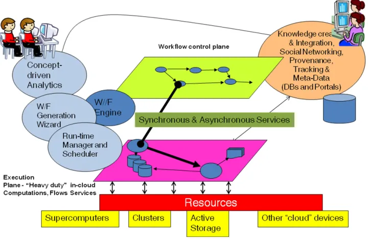
Kepler workflows often operate on the “control plane.” Figure 1.1 illustrates this.

Figure 1.1: Illustration of the control plane orchestration of workflows and resources.

In a Kepler workflow, a process is called an actor. Actors are interconnected by

(16)

3 representation is offered by a graph. Execution of the whole workflow can have two parts –

execution on the control plane (Kepler, Figure 1.1) where actors act as flow routers and

intermediaries that manage real resources on supercomputers, dedicated clusters and in the

cloud. Such a workflow is controlled by one of a number of special schedulers called

Directors. SDM has also developed a provenance collection framework for Kepler [4], along

with visual interfaces to display and analyze the results – the dashboard [5]. This is illustrated

in Figure 1.2

Figure 1.2: SDM framework that support provenance data collection, workflow management through a dashboard, and a Kepler orchestration engine.

1.2 Challenges facing Scientific Workflows

Scientific Workflow Management Systems (S-WFMS) have proven to be a valuable tool in

(17)

4 analysis and visualizations [6]. As workflows become more complex, they also become more

vulnerable to internal and external failures requiring fault tolerance during workflow

execution [7] [8].

While classical fault tolerance solutions can operate well in the context of modern scientific

workflows, some limitations arise from the nature of the scientific workflow engines,

characteristics of workflow models, and the failure rates and bounds that application domain

is willing to tolerate. Scientific workflows may include long-running, loosely coupled and

repetitive computational steps that require the tolerance of failures during run-time with

minimal impact on the overall execution. Fault tolerance approaches to scientific workflows

should provide run-time failure avoidance and/or mitigation within workflow models and at

different levels of an execution infrastructure. They also should be able to adapt to workflow

evolution and to changes in its operational environments.

1.3

1.4 Publications

A considerable amount of work discussed in this dissertation has been published by the

author of the dissertation in the form of papers, tutorials and posters. For example, fault

tolerance as it relates to scientific workflows is discussed in [9] [10] [11] [12]. Provenance

management is scientific workflows is discussed in [13] [14]. Dashboard and simulation

monitoring are discussed in [15] [16] [17]. Scientific workflows and their role in the

(20)

7

Chapter 2

Failure Rate Analysis

2.1 Definition of failure

In order to understand the problem, let us start by formally defining the meaning of “failure”

[22].

“An error, or a mistake, made by a human or an external entity results in a fault in a software or system artifact1 (e.g., missing or extra instructions in the code, wrong input

settings, requirements or other documentation omissions, etc.). This fault can propagate

through subsequent software stages and artifacts as one or more defects. When software is executed and encounters such a defect, it may go into an error-state. If an error-state results in an observed departure of the external result of software operation from software

requirements or user expectations, we say that we have observed a failure of the software/system. Failures also can be caused by error-states that arise from lacks in user's

knowledge and training (how-to-use-errors) and through resource exhaustion (e.g., out of disk space exceptions, hardware failure) that may or may not be properly handled by

the software or the system. Failures and their frequency, tend to relate very strongly to

customer satisfaction and perception of the product quality. Faults, on the other hand, are

(21)

8 more developer oriented, since they tend to be translated into the amount of effort that

may be needed to repair and maintain a system. Fault tolerance mechanisms try to

prevent, or at least minimize, adverse impacts of failures. They can do that in a number of

ways through forward recovery (e.g., masking of error-states, redundancy with voting

mechanisms), and backward recovery (e.g., checkpointing, state recovery and

re-execution)”.

2.2 Failure rates in HPC systems

High performance computing systems, especially supercomputers, such as the ones available

at Oak Ridge national laboratory [15], provide an invaluable tool for scientific research and

discovery. However those systems are very expensive to own and maintain, and failures

related to those systems can be very costly. Therefore studying and analyzing failures in such

systems can improve reliability, and thus productivity, by better resource allocation and

management [24].

There are several studies of failures in high performance computing systems, e.g., [25] and

[26]. However, they are based on a few months of data at most, covering a small number of

failures, and are relatively outdated. In 2005, Los Alamos National Lab released the raw data

on failures that has been collected over a period of nine years [27], and in 2006, NERSC

released the error data on I/O related failures collected over a period of 5 years [28]. Several

(22)

9 These studies concluded that failure rates vary widely across systems, ranging from 20

failures to more than a 1000 failures per year, depending mostly on the system size (for

example, systems with 4096 processors averaged 3 failures per day). Furthermore, they find

that failure rates are linearly proportional to the number of processors per system.

Looking at the root causes of the failures, we noticed that around 50% were hardware related,

20% user related, 20% had unknown origin, and the remaining 10% split up among network,

software and environment. As for the time to repair, the study finds that it varies between less

than 3 hours and more than 10 hours, based on the type of error, with a mean time to repair of

355 minutes.

(23)

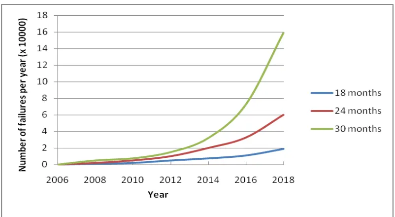
10 Figure 2.1, based on data from [29], shows the expected growth in failure rate as the size and

complexity of supercomputers increases, and assuming that the number of cores will increase

by a factor of 2 every 18, 24, or 30 months respectively. As the number of devices

(processors, disks) increases, assuming no additional built in recovery mechanisms, so does

the likelihood that the system is out of service for one reason or another. Furthermore, as the

cost of those systems increases, those failures become very expensive. Therefore failure

handling and reliability play a vital role in making systems scalable.

2.3 Failure rates in scientific workflow management systems

Both tightly coupled and loosely coupled systems become more failure prone as their size

and complexity increases. Some systems, such as those found at ORNL, LANL and NERSC,

are expensive, high priority, tightly controlled and closely maintained systems. They benefit

from such additional close scrutiny. On the other hand, Grid based computational systems,

such as the TeraGrid [31] and more recently cloud-based systems, may be more susceptible

to failures due to the diverse and general-purpose nature of such infrastructures. The

heterogeneous computing systems that make such grids, which are often loosely coupled by

grid middleware, are much harder to monitor and control and therefore mitigate its failures.

Failure rates among grid based workflows vary greatly. This is due to factors such as the size

and type of the workflow, the type and amount of resources it consumes, and the duration of

(24)

11 For example, the authors in [32] describe the workflow system LEAD (Linked Environment

for Atmospheric Discovery) which is used to study weather forecasting. Over a period of a

month, 165 workflow runs were executed, with a total of 865 workflow steps [33]. Out of the

165 workflows 131 failed, due to a multitude of reasons mostly relating to errors that

occurred in the grid infrastructure. That is a 78.8% failure rate, which meant that failures are

the norm rather than exception. The authors later present a retry mechanism for their

workflows which reduced the failure rate to approximately 23%, which is a large

improvement; however that is still a large failure rate.

Another example is the work reported in [34], in which the authors studied the reliability of

two grid platforms, TeraGrid [31] and Geon [35] via a deployment of a monitoring and

benchmarking infrastructure. They conclude that the failure rates vary between 20% and

45%, based on the type and length of the test used.

2.4 Failure rates in Kepler based scientific workflows

2.4.1 Production level workflows use cases: XGC and S3D

In this section we discuss two use cases of production workflows that are used at Oak Ridge

National Laboratory, and Sandia National Laboratory. We also discuss some use cases to

describe some of the most commonly encountered errors.

XGC [36] [37] and S3D [38] are numerical simulation codes that scientists at the ORNL and

(25)

12 respectively. Kepler-based workflows, e.g. [39], have been developed for both of these codes

to automate the processing steps involved in deploying these codes on a supercomputer and

analyzing the outcomes of the runs.

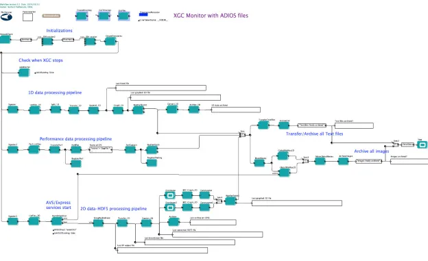
The XGC monitoring workflow is shown in figure 2.2 below, and the S3D workflow is

shown in figure 2.3. These workflows might appear to have parallel execution flows, but

effectively it is a serial flow, since the execution eventually blocks waiting on all the

(26)

(27)

(28)

15

2.4.2 Typical failure scenarios

Both workflows are part of a family of workflows, that involve similar steps, known as

deployment and monitoring workflows [40]. After computational codes have been launched

on a supercomputer, these workflows monitor and manage outputs from long-running

computations. Tasks include movement of data files to an analysis computer, archiving of the

data, and generation of visualizations based on the progress of the computations. Due to their

similarity, these workflows also exhibit similar categories of failures. Currently, both

workflows also have an ability to effect some recovery from a failure through a light-weight

start option – a feature that keeps track of successful task executions and does not

re-execute them on re-start unless it is required by the task pipeline [41]. Below, we provide

scenarios that highlight possible failures within these scientific workflows.

Scenario 1: Scientific workflows commonly access a diverse set of resources such as web services, databases, and external applications. A maximum time limit is often set when

accessing these resources since they, or the networking link to them, may fail or become

unresponsive. When this limit is exceeded and a timeout occurs, how should workflow

execution proceed?

For example, the XGC workflow executes several applications to generate visualizations.

When a timeout occurs in that part of the workflow, the workflow considers that this step has

been completed “successfully,” but no images or movies are produced. This may not always

be a desirable way to handle such a failure, but it is probably the most expedient one in this

(29)

16

Scenario 2: Kepler workflows often have long chains of actors linked together forming processing pipelines. If a failure occurs while executing one of these tasks, what actions, if

any, should be performed for the remaining tasks?

Figure 2.4: Failure in Processing Pipeline [12]

This situation is illustrated in Figure 2.4. It can occur in the S3D workflow [38], and the

resulting actions depend on the state of the actor that failed and on downstream actors. If

there is a failure in the second task, some of the subsequent activities should not be executed

(denoted by the red arrows) as they can crash the overall workﬂow. However, other tasks

(denoted with the green arrows) should be executed since their outcomes are necessary for

the remainder of the workﬂow. This is currently a difficult design to implement as a

workflow since the green activities cannot be gathered in an alternative path in a systematic

manner due to inconsistencies of input/output types or their structuring over different paths.

In this case, the fault tolerance takes on the challenge of structuring the tasks on conditional

paths for every possible failure, input/output match and consistent precedence order. This

(30)

17

Scenario 3: Scientific workflows rely on a multitude of middleware services to successfully run a simulation. For example, the XGC workflow uses services for data manipulation, data

transfer, visualizations, etc. These services are not a part of the workflow and therefore, are

not monitored or controlled by the workflow; they are simply invoked from the workflow

layer. What happens if one of these services becomes unresponsive and the workflow layer

does not realize it until it is too late, or not at all? In either case the normal execution of the

workflow is disrupted. How does one handle that? In the current workflow implementation,

that would lead to a failed run, which would have to be restarted after the workflow scientist

addresses the underlying problem. That is very inefficient since those run can take hours to

complete, and restarting a run after it fails is time and resource consuming.

2.4.3 Fault classification

Analysis of workflow failures shows the range of issues that fault tolerance mechanisms need

to handle in our case. Based on a logs of more than 1000 production runs of XGC and S3D

workflows at ORNL collected between February 2009 and April 2010, (refer to Appendix A

for sample production run log files), the failures and error-states encountered are summarized

in table 2.1. Note that many failures are transparent to the workflow, and thus do not

interrupt normal workflow execution. Unfortunately, in those cases, even when the workflow

finished successfully the underlying simulation results were invalid.

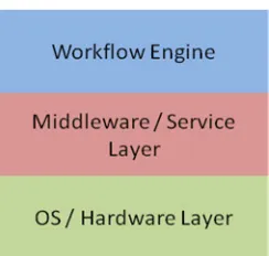
Problems listed in table 2.1 can be classified based on which layer of the execution

environment they originate. Figure 2.5 depicts three execution layers: the Workflow Layer

(31)

18

Middleware Layer provides all services required for executing the simulation; and the

Hardware/OS Layer is where the simulation codes run, data are stored, etc. A failure or an

error-state occurring at one layer can propagate causing additional issues.

To better understand those errors, let us consider the log files of the failed run in Appendix

A.2. The first failure encountered at line 43 was caused by “bpappend” due to a missing path

in the environment variables of the cluster. The missing path caused all “bpappend” and

“bp2h5” operations to fail, therefore no images were generated, which resulted in the

visualization job (AVS) failing to start, leading to a workflow execution failure. Note that the

first failure was encountered only 1 minute after the execution has started, and yet the

workflow ran for 52 minutes before it was halted due to the failures.

For the classification in table 2.1, we only list the descriptions of what we consider the

root-cause of failure for each failed run, and not all the failures encountered during that run. For

example, the run listed in Appendix A.2 would have the root cause classified as “missing

(32)

19 Table 2.1: Root-cause analysis

Description Faults %

Total Nb of faults encountered System(s) on which Failure Occurred Example

Deadlock 5% 4 All Workflow Design Error causing deadlock

Missing

Modules/Libraries/Paths 12% 11

Supercomputer Analysis Cluster

Incorrect Path on cluster (example run in Appendix A.2)

Data Movement Failure 8% 7 All Moving data files across cluster fail or

checksum incorrect

Incorrect Input 8% 7 Staging Cluster User entered incorrect workflow parameters

Incorrect Output 9% 8 Supercomputer File generated are corrupted

Authentication Failed 7% 6 All Archive command failed because the HPSS

authentication was unsuccessful not work

Job Submission Failed 4% 4 SuperComputer Job not added to queue

Service not Reachable /

Responding 6% 5 Analysis Cluster AVS died

Node Crash / Down 8% 7 All Supercomputer restarted and workflow lost

connection

Network Down/Error 4% 4 All Network outage caused the workflow to lose

connection with the SuperComputer

Out of Disk Space 2% 2 Analysis Cluster Partition was full, files could not be written

CPU time limit exceeded 10% 9 SuperComputer Time reserved for simulation insufficient

File Not found 10% 9 SuperComputer

Analysis Cluster Data files were placed in wrong location Other (Out of Memory, Job

Stuck in Queue, Uncaught Exception…)

7% 6 All Job priority too low and not executed.

(33)

20 Figure 2.5: Execution Environment Layers

Run-time failures can be quite expensive. For an XGC monitoring workflow [36], the

workflow runtime can vary between two and ten hours depending on the simulation with

about 2/3 of the time being spent on supercomputers. We found that on the average XGC

workflows fail about 9% of the time, wasting up to 7% of allocated supercomputing time.

When one considers more complex situations, such as coupled workflows [39], where two

different simulations exchange information, and/or one workflow controls both the

simulation and the analysis, and the runtime can be as long as two days, workflow failures

becomes even more of an issue.

(34)

21 Figure 2.6 provides a layer-oriented analysis of the data in table 2.1. Notice that nearly 70%

of the originating issues occur either at the Hardware/OS layer or the Middleware layer.

These error-states/failures can be difficult to detect. Also, in our experience, most of the time

they do not propagate to the workflow layer in time, or with sufficient information attached,

for the workflow to actively address the impact and resume execution. Therefore,

workflow-level fault tolerance mechanisms need to be supplemented with methods that actively

monitor lower layers and communicate adequate information to the workflow-layer in time

for a recovery action to take place.

Now let us consider the different types of resources/clusters used for our workflow

executions, and the time spent per run on each resource. For simplicity we will assume an

average workflow runtime of 6 hours. The resources can be divided into 3 categories:

1. The staging cluster: A small sized cluster with 32 nodes. It is responsible for

launching the workflow, preparing the scripts and input files, and submitting the job

to the supercomputer. Then monitor for output files, and transfer them to the

processing cluster. Around 10% of the workflow run time is spent at this stage, so

considering an average running time of 6 hours, the time spent on this cluster is

approximately 36 minutes.

2. The supercomputer: The majority of the workflow run time, around 70%, is spent on

the supercomputer. That means approximately 252 minutes out of our 6-hour

simulation runtime is spent at this stage. The supercomputer currently being used is

(35)

22 3. The analysis and visualization cluster: Approximately 20%, or 72 minutes, of the

6-hour simulation time is spent analyzing and visualizing the data. This cluster is made

of 162 nodes.

2.4.4 Failure Analysis

Figure 2.7 below represents the proportionally projected average run time per computing

resource based on the overall run time of production workflows. For the workflow runs

examined, the run time ranges between two and ten hours. Notice that over 50% of a

simulation run time is spent on the supercomputer.

Figure 2.7: Average run time per Computing Resource based on the total run time

Figure 2.8 shows the percentages of failures and the time they occur based on the examined

(36)

23 at the staging cluster, the red bars represent the failures that occurred on the supercomputer,

and finally the green bars represent the errors that occurred on the analysis cluster.

Figure 2.8: Time of failure occurrences

The failure percentages shown in figure 2.8 map onto the root causes which lead the

workflow to fail either at that time, or later during the run. For example, a failure occurring at

minute 228 might cause the workflow to halt then, at a later time, or it might not halt the

workflow at all. In the last case, this means it will be up to the end user to detect it. For

simplicity, we will consider that the time of at which failure occurs is the time when the

workflow halts.

If we take as example a workflow with runtime duration of 6 hours, based on figure 2.7, the

workflow would run on the staging cluster for 36 minutes, on the supercomputer for 252

minutes, and on the analysis cluster for 72 minutes. Now based on the failure rates noted in

(37)

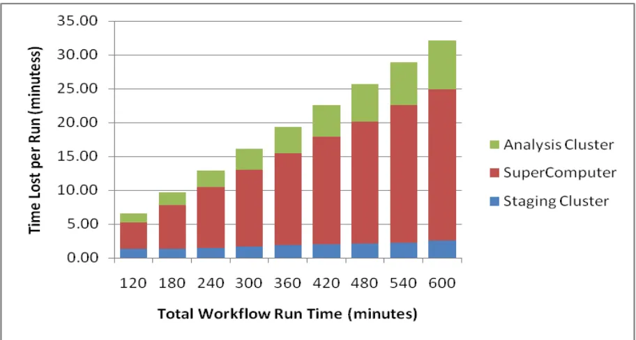
24 lost per workflow run (by taking the total run time of successful and failed runs and dividing

by the number of successful runs) to be 1.93 minutes on the Staging Cluster, 13.54 minutes

on the supercomputer and 3.87 minutes on the analysis cluster for that particular run.

Finally let us consider the average time lost per workflow run based on the duration of each

run. As we mentioned earlier, the runtime ranges between two and ten hours, but as more

complex workflows are introduced, the run time will go up, lasting up to several days. Figure

2.9 below shows the average time lost per run based on the duration of the run (calculated by

taking the total run time of successful and failed runs and dividing by the number of

successful runs).

(38)

25

Chapter 3

Fault Tolerance mechanisms in scientific

workflow management systems

3.1 Overview

This chapter presents an overview of the most commonly used scientific workflow

management systems and their fault tolerance capabilities. A large percentage of these

workflow management systems are grid based and generally rely on fault tolerance

capabilities presented by the Grid framework. The fault tolerance capabilities of scientific

workflow management systems can be divided into two main categories: 1) checkpointing

based fault tolerance, and 2) Retries and/or alternative versions based fault tolerance.

3.2 Checkpointing

Checkpointing is defined as storing recovery information of a process, so that in case of a

failure, the process can be restarted from the last saved state [42]. The recovery information

includes the states of sub-processes, and the intermediate data and meta-data generated.

(39)

26 The same basic principles apply to scientific workflows. In the case of Kepler, the

sub-processes are actors within a workflow, and the intermediate data or meta-data is generated

and consumed by each actor. Below is a list of the most commonly used workflow

management systems that support checkpoint based Fault Tolerance, and their limitations.

1. DAGMan. DAGMan [43] is a meta-scheduler for Condor [44]. It manages dependencies between jobs at a higher level than the Condor scheduler. DAGMan bridges the scientific

domain and the execution environment by automatically mapping the high-level

workflow descriptions onto distributed infrastructures. Several workflow management

systems use DAGMan, such as Pegasus (Planning for Execution in Grids) [45] and

P-Grade [46].

DAGMan offers a checkpointing based fault tolerance mechanism [47] which benefits all

the scientific workflow management systems that use DAGMan as a scheduler. With the

help of DAGMan, workflows can recover from machine crashes and network failures.

They can detect authentication errors, idle staging job submission faults, job crashes,

input unavailability and data movement faults. Recovery is effected with the help of

DAGMan’s Rescue DAG [48]. When the workflow abnormally terminates, a Rescue

DAG is generated containing the tasks not yet finished. By executing the Rescue DAG

instead of the original workflow, successfully completed portions are not re-executed.

(40)

27 workflows. It uses Karajan [50] for execution engine and Falkon [51] for job

submissions. Swift stores a “restart log” of workflow executions, allowing it to resume

the computation in case of an early termination. They extend the rescue-DAG approach

using cashing strategies, by storing and reusing the computation results of previous

workflow components invocations.

3. Askalon. Askalon [52] is an open source workflow management system that provides a set of high-level services for transparent Grid access, including a sophisticated scheduler

for the optimized mapping of workflows onto the Grid. Askalon provides workflow level

checkpointing and migration, in which it saves the workflow state and the intermediate

data at the point when the checkpoint is taken. It then allows the execution to be resumed

on either the same grid resources or migrating the workflow to different grid resources.

4. Trident. Trident [53] is a scientific workflow management system developed at Microsoft Research. Trident provides a workflow level checkpointing mechanisms. It

allows the user to restart a failed workflow from the last successful checkpoint, and gives

the user the option to allocate different resources for that workflow restart, similar to the

migration option available in Askalon.

(41)

28 extension to LEAD in which they provide Fault Tolerance support using checkpointing

and migration.

6. Others. Several other workflow management systems provide similar checkpointing capabilities. For example the authors in [55] present a checkpointing mechanism that

incrementally records the state changes which can be undone in a rollback in case of a

fault. However this solution can only be used at runtime and doesn’t provide persistent

state storage for a full restart after a workflow crash.

The authors of [56] present another checkpointing mechanism that saves the intermediate

results at the middleware level, by extending the anthill [57] execution engine. In [58], the

authors present a workflow level checkpointing mechanism in which every workflow node

creates its own local checkpoint autonomously after its enactment.

3.3 Fault tolerance based on Retries and Alternative Versions

The notion of Retries/Alternative Versions [59] [60] recovers from a failure in the execution

by either re-executing the failed step, or by executing an alternative version of the failed step.

This also includes the execution of alternate versions in parallel with the hope that at least

one version would deliver a valid result. Alternative versions can be either identical, or they

(42)

29 These notions have been applied to several occasions to scientific workflow management

systems. Below is a list of the most common ones.

1. Pegasus. As we mentioned earlier, Pegasus (Planning for Execution in Grids) [45] relies on DAGMan for checkpointing capabilities, but it also offers workflow level redundancy

using retries, resubmission and task migration.

2. Taverna. Taverna [61] features a three-layered architecture: The “application data flow” layer provides a user’s perspective of a workflow, hiding the complexity of interoperation

of services; the “execution flow” layer is responsible for workflow scheduling, service

discovery, data, and metadata management; and the “processor invocation layer” is

responsible for the invocation of concrete services. Fault tolerance support in Taverna is

limited to retries and alternative versions [62] at both the services level and the workflow

level. Several retry types are supported such as exponential back-off of retry times.

3. Triana. Triana [63] is an open source problem solving environment. It combines an intuitive visual interface with powerful data analysis tools. It is used by scientists for a

range of tasks, such as signal, text and image processing. Triana includes a large library

of pre-written analysis tools and the ability for users to easily integrate their own tools.

Support for fault tolerance is generally user driven and interactive in Triana. For

example, faults will generally cause workflow execution to halt, display a warning or

(43)

30 Machine crashes, network errors, missing files and deadlocks are recognized by GridLab

GAT [64] and the Triana engine, respectively, but recovering from or preventing them is

not supported. Data movement and input availability errors are detected by the Triana

engine but are not recoverable. Workflow level light-weight checkpointing and workflow

restart are currently supported.

4. P-Grade. P-Grade [46] supports retries and resubmissions with the help of its resource and task manager (gLite [65]). It also supports light weight checkpointing at the

workflow level.

5. Askalon. Askalon [52] supports recovery of certain types of errors such as data movement faults, unavailable input data, failed authentications and a few others.

However it does not support user defined exceptions in its current version.

6. Swift. Among the middleware components that Swift [49] relies on, it also uses Globus services [66] which inherently provide fault tolerance capabilities to Swift such as retries

and execution migration. Beyond that fault tolerance support is limited to checkpointing

at the middleware level.

(44)

31 8. Others. There are several other common scientific workflow management systems, such as VisTrails [67], Escogitare [68], and View [69]. They offer similar capabilities to other

WFMS, but each is adapted to a particular science niche and depends on different types

of infrastructure. Vistrails is an open-source scientific workflow and provenance

management system that provides support for data exploration and visualization. It is the

first system that supports provenance tracking of workflow evolution in addition to

tracking the data product derivation history. Escogitare is used for bioinformatics and

geoinformatics experiments and uses the BPEL language [70] for describing workflows.

Most of these systems provide partial fault tolerance support, either by the workflow

system or the underlying infrastructure. For example, Escogitare mainly relies on the

.catch. operation of BPEL [70] to handle certain types of errors. View presents a task

level exception handling language, which defines the alternatives to be executed in case

of a failure of a specific task, similar to our previous work described in [9].

3.4 Summary

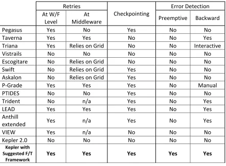
Table 3.1 below lists the scientific workflow management systems mentioned above and

summarizes the fault tolerance capabilities of each of those systems. Note that Kepler, in its

current release (2.0), does not support any fault tolerance capabilities, and current failures are

addressed on a case by case scenario by the developers. In order for Kepler to remain

competitive with other scientific workflow management system, it needs to be extended to

provide such capabilities. The last entry in table 3.1 represents the extended capabilities of

(45)

32 Table 3.1: Scientific Workflow Management Systems F/T Capabilities

Retries

Checkpointing Error Detection At W/F

Level Middleware At Preemptive Backward

Pegasus Yes No Yes No No

Taverna Yes Yes No No Yes

Triana Yes Relies on Grid No No Interactive

Vistrails No No No No No

Escogitare No Relies on Grid No No No

Swift No Relies on Grid Yes No No

Askalon No Relies on Grid Yes No No

P-Grade Yes Yes Yes No Manual

PTIDES No No Yes No No

Trident No n/a Yes No Yes

LEAD Yes Yes Yes No Yes

Anthill

extended Yes n/a Yes No Yes

VIEW Yes n/a No No No

Kepler 2.0 No No No No No

Kepler with Suggested F/T

Framework Yes Yes Yes Yes Yes

As mentioned earlier, most of the workflow management systems are grid based and they

mostly rely on middleware grid services for fault tolerance support. Note that none provide

preemptive failure detection, and there is limited backward detection, i.e., he ability to

determine the failure source once an error has occurred. Our framework, discussed in

(46)

33

Chapter 4

Kepler provenance framework

4.1 Description

The Kepler provenance framework [4] was developed to help analyze and process the data

generated by Kepler workflows. The provenance data recorded are also used by the fault

tolerance framework as discussed in the following sections. Following is a brief overview of

the different types of provenance and of the Kepler provenance framework [13] [14].

Data provenance refers to the origin and the history of the data and its derivatives (meta-data). It can be used to track evolution of the data, and to gain insights into the analyses

performed on the data. Provenance of the processes, on the other hand, enables scientist to obtain precise information about how, where and when different processes, transformations

and operations were applied to the data during scientific experiments, how the data was

transformed, where it was stored, etc. In general, provenance can be, and is being collected

about various properties of computing resources, software, middleware stack, workflows

(47)

34 Figure 4.1: Provenance framework

The Kepler provenance framework developed by the SPA team is illustrated in figure 4.1. At

the core is the provenance database with its APIs. The generality of the design allows

insertion of another database (or another storage option) of choice. API has three key

components: (1) Kepler, its actors, and external scripts use a Recording API to collect and save provenance information; (2) a Query API provides different query capabilities for dashboards, query actors in Kepler, and SQL statements; and (3) a Management API for Provenance Store maintenance. Currently, recording API is actually part of the Kepler.

The database stores all provenance information. The architecture has one important

requirement of the database: it must be self-contained, but it can be distributed. Simple items

like annotations, user identifiers, timestamps, etc., are stored in closely corresponding SQL

data types, such as numeric or varchar. More complex items are stored as BLOBs. For

(48)

35 Object. In this case, if the user wishes to save all tokens produced by the actors in his

workflow, he/she would need to provide serialization routines to store and retrieve the

relevant Java Objects. An alternative is to use database stored pointers to reference the

provenance information outside the database, such as Java Objects or workflow configuration

files, pictures, movies or application source code. However, this solution may require a

mechanism to reference data across machine boundaries. Self-containment guarantees that

modifications to provenance information are done only using the Provenance Store

Recording API, and that full set of information is preserved.

The Kepler workflow management system implements a Provenance Recorder. It is a set of

listeners, or hooks – that saves token-based provenance from all (internal) workflow

components into the Provenance Store. Depending on the granularity, that data may be

recorded for all actors in the workflow, or some subset, e.g., only top-level composites. The

recording API additionally supports input from components external to Kepler. These components are usually Python or shell scripts called by actors running in a workflow.

Furthermore, these scripts may execute on a machine other than the one running Kepler. An

example is the performance parameters that may come from software instrumentation and

performance tools. In this dissertation we are particularly interested in the information stored

about actor firings and tokens, which is the basis of the analysis routine mentioned later.

(49)

36 recorded (e.g., a web based dashboard) to querying details about past executions. In addition

to providing current workflow status, applications can query the Provenance Store about past

executions. The Query API contains an SQL interface to support these types of queries; it can

retrieve data from the database given appropriate authorization. Finally it also provides a

callback mechanism for applications wishing to receive real-time provenance updates.

The management interface provides user administration and maintenance operations. User administration includes, adding and deleting users, modifying user passwords, modifying

user access rights, and specifying the set of accessible workflows.

Security of the system has always been of importance. For example, in the current context of its use, the challenge is automated communication and exchange of data with other

government labs. We are in the process of implementing a certificate-based security envelope

that will allow inter-laboratory exchanges. Furthermore, we are increasingly concerned about

the sharing of the provenance data. We realize that workflow meta-data and provenance

information may have as much value as the raw information. Typically, sensitive information

produced by a computational processes or experiments is well guarded. However, this may

not necessarily be true when it comes to provenance information. The issue is how to

appropriately share confidential provenance information. We developed a model for sharing

provenance information when the confidentiality level is dynamically decided by the user

(50)

37

4.2 Provenance database

Figure 4.2 shows the provenance database schema used by the Kepler provenance recorder.

Figure 4.2: Provenance database schema

The provenance framework records the provenance data for all the entities of a workflow as

shown in the database schema. This includes recording the director parameters, the actor

parameters, firings, ports, tokens generated and consumed, etc. For the purpose of this

dissertation, we are particularly interested in the tokens generated and consumed, since they

will help us establish a lineage of the execution, and create an execution flow. This is

important for the Checkpointing solution presented in chapter 6 because it will help us

re-populate the actor queues based on the last successful checkpoint. This will be discussed in

(51)

38

4.3 Token tracing

In general the amount of data collected by the Kepler provenance framework is large and

grows significantly with the size and complexity of the workflow. Usually the information of

interest is only a small fraction of what’s being collected. Having the scientists search

through that data is time consuming and negates the purpose of data provenance meta-data,

therefore the need for automated, flexible and extensible mechanisms for mining the

provenance data.

For example, if a scientist wishes to further investigate or analyze an image that was

generated by the workflow, he/she may need to first locate the file that contains the data

behind that image. This is not an evident task since a single run can have hundreds of images

associated with it. Furthermore, the relationship between images and the data files may not

be one-to-one. This means that one data file may contain the data for several images.

Consequently the scientist needs to both locate the data files on the disk, and to examine the

contents of the data files before it can be determined which one contains the data of interest.

That can generate a lot of overhead, especially for complex workflows such as those

discussed in section 2.4.1 which has multiple codes integrated in it.

To illustrate and discuss development of provenance analysis algorithms and their insertion

in to our Kepler-based provenance framework we will use image data files and archived data

(52)

39 The challenge is to identify and track the data files that generate images displayed on the

Dashboard [5]. The solution developed checks the tokens generated and consumed, and

creates a reverse graph of the token flow, starting with the image name, and ending with the

data file(s). However tracking archived files was more challenging because the token trace is

not linear when tracing forward through the branching trees. Instead of tracing backwards,

we need to trace forward through the branching trees. Figure 4.2 below details the different

steps required for successfully finding an archived data file.

Figure 4.3: Tracking Archived Data Files [13]

The work presented in this section is being included in this dissertation because it explains

how the token trace is established. This solution was developed to track the data files

(53)

40 checkpointing based restart. The upcoming sections shall discuss in detail the role the

(54)

41

Chapter 5

Forward Recovery

5.1 Motivation

The environment in which workflows under consideration here execute can be divided into

three layers: The workflow layer, the middleware layer, and the OS/hardware layer. The

workflow layer, or the control layer (figure 1.1), is the driver behind the wheel providing

control, directing execution, and tracking the progression of the simulation. The framework

we are proposing has three complementary mechanisms: a) a forward recovery mechanism

that offers retries and alternative versions at the workflow level, b) a checkpointing

mechanism, also at the workflow layer, that resumes the execution in case of a failure at the

last saved good state, and c) an error-state and failure handling mechanisms to address issues

that occur outside the scope of the Workflow layer. This chapter describes the first

component if that framework, the Forward Recovery mechanism. Chapters six and seven

describe the remaining two components.

Forward recovery mechanisms attempt to compensate for failures and keep the workflow

execution going without a major externally visible interruption such as re-execution of the

(55)

42 example by checking execution results for correctness. There are two main approaches to

detecting error-states caused during execution faults:

(i) Acceptance testing of the results via executable assertions [59]. An acceptance

test may determine functional equivalence, or may determine correctness

measured against an always-correct result, and

(ii) Use of alternate version(s) [59] [60]. Alternate versions execute in parallel and

each delivers a result. Alternative versions can be either identical, or they can be

independent versions that are functionally equivalent.

Results delivered then need to be compared to determine which one is correct, and then either

the correct result is passed on to the rest of the workflow, or a “graceful” failure exit needs to

be taken. The best-documented techniques and most commonly used for tolerating faults in

software-based systems are the Recovery Block (RB) approach [60] and N-version

programming (NVP) [72] In either case, there needs to be a decision mechanism which deals

with the situation where it may not be possible to recover from a failure. In this case one also

has to worry whether failures that might occur are correlated or not. Correlated failures can

reduce effectiveness of the failure or error-state detection mechanisms [59].

5.2 Contributions

The main contribution of this part of work is a Retry/Alternative Version mechanism for the

Kepler workflow management system. Although principles have been known for some time

and have been extensively studied in the literature, the contribution here lies in adapting

(56)

43 complement the other fault tolerance mechanism discussed in the next two chapters, in order

to present an entire fault tolerance framework that would address most if not all of the errors

encountered in our production workflows.

5.3 Architecture

5.3.1 Overview

To implement the forward recovery part of the whole strategy, we develop a Contingency Actor. Its early predecessor – fault-tolerant web-services actor is discussed in [8] along with performance gains that can be achieved assuming failure independence. Several

sub-workflows may be associated with this actor: one sub-workflow represents the primary set of

tasks to execute. When a failure occurs, this sub-workflow can be re-executed with the

original inputs if we believe that the failure is a transient one, or an alternative sub-workflow

can be executed instead. Furthermore, the actor may pause the execution between

sub-workflow executions if some other action needs to be taken. This work was implemented

jointly by the SPA team at North Carolina State University and San Diego supercomputing

center (SDSC) and was published in [12].

5.3.2 Workflow interface

Figure 5.1 shows an example configuration of the contingency actor. The primary task,

implemented in a sub-workflow, called “primary-ssh”, is to ssh to a server and execute a

script. This sub-workflow is shown in Figure 5.2 with the alternative sub-workflows

(57)

primary-44 ssh sub-workflow three times, waiting five minutes between each attempt. If the connection

cannot be made after the final attempt, a secondary sub-workflow, “secondary-ssh,” is run,

which ssh-es to a different server. If this fails, the contingency actor runs the third

sub-workflow, “email”, which notifies the user and the workflow fails.

Figure 5.1: Example contingency configuration

Figure 5.2: The primary-ssh sub-workflow in the contingency actor

When the contingency actor receives new input from upstream actor(s) for the first time, it

executes the primary sub-workflow. The user chooses the first (primary) sub-workflow to

execute: it may either be the same sub-workflow each time, or the last successfully executed

sub-workflow. In the previous example, ”primary-ssh” should always be tried first since the

script runs faster on that server. However, if this server is often unreachable for long periods

(58)

45 secondary server. In this case, contingency can be configured such that if “primary-ssh” fails

but “secondary-ssh” succeeds, subsequent input will execute “secondary-ssh.” Furthermore

the knowledge of which sub-workflow to execute first may be shared among multiple

instances of the contingency actor within a single workflow.

5.3.3 Monitoring layer plug-in

To better help the contingency actor decide which alternative to choose, by determining

which one has the highest rate of success, we provide an interface over which it can

communicate with other components of the presented fault tolerance framework, namely the

monitoring layer and the provenance database. The monitoring layer and the interaction

between it and the contingency actor are discussed in detail in chapter 7.

5.4 Error-state handling

One of the classical failures is resource timeouts. Below is a simple example of how the

contingency actor can address timeouts by retries or, if all alternatives fail, by pausing the

workflow and notifying the user. The sequence diagram in Figure 5.3 below shows how the

contingency actor can be configured to automatically increase the timeout and re-execute the

(59)

46 Figure 5.3: Automatic retry with increased timeout

A user starts the workflow which at some point invokes the contingency actor. The primary

task of contingency executes the script with a timeout of one minute. When this timeout is

exceeded, the script aborts and notifies the contingency actor. The contingency actor’s

secondary task then increases the timeout to five minutes and re-executes the script. The

timeout is not exceeded, and the script successfully completes. The workflow then executes

the remaining actors and eventually stops.

Figure 5.4 shows another scenario where the timeout parameter may be specified in the

external application and not available to the workflow layer. When a timeout occurs in these

situations, our architecture can notify the user, gracefully stop workflow execution, and

(60)

47 Figure 5.4: Notify user and smart resume [12]

As in the previous solution, a user starts the workflow, which eventually executes the

contingency actor. In this solution, the primary task executes the script without a timeout

value (specified in the workflow layer). When a timeout occurs, contingency’s secondary

task sends email to the user describing the problem, and stops the workflow. Once the user

has increased the timeout in the script, she re-executes the workflow. During initialization,

(61)

48 The contingency actor’s primary task executes the script, which completes successfully. The

workflow then runs to completion.

Yet, another scenario is when a failure occurs executing a task which would cause

subsequent tasks to fail, thus those subsequent tasks should be not executed since they may

crash the workflow. Figure 5.5 explain how this scenario is addressed using the contingency

actor.

Figure 5.5: Embedded Tasks in Contingency Actors [11]

The tasks that always execute (green arrows) are unmodified, but tasks that should not be

executed if an error-state occurs (red arrows) have been embedded in contingency actors.

Each contingency instance contains two sub-workflows: Task A executes if there are no

error-states, and task B executes when an error-state occurs. For this use case, task B is an

empty sub-workflow that simply passes input data to the next task. If an error-state occurs

while executing task A in the first contingency actor, task B executes. In subsequent

contingency actors, task B executes instead of task A, preventing the workflow from

(62)

49

Chapter 6

Checkpointing

6.1 Motivation

Another approach for providing fault tolerance through backward recovery is checkpointing.

Checkpointing principle is a widely used and consists of storing a snapshot of the current

application state, and using it for restarting the execution in the case of a failure [73]. There

are many ways for achieving application checkpointing. Depending on the specific

implementation, a checkpointing tool can be classified by:

a) Amount of state saved: This refers to the abstraction level used by the technique to

analyze an application. It can range from seeing each application as a black box,

hence storing all application data and state information, to selecting specific relevant

core data in order to achieve a more efficient and portable operation.

b) Automatization level: Depending on the effort needed to achieve fault tolerance

through the use of a specific checkpointing solution.

c) Portability: Whether or not the saved state can be used on different machines to

restart the application.

d) System architecture: How is the checkpointing technique implemented: inside a