University of Windsor University of Windsor
Scholarship at UWindsor
Scholarship at UWindsor
Electronic Theses and Dissertations Theses, Dissertations, and Major Papers
2009
Video Super Resolution
Video Super Resolution
Michael Chukwu University of Windsor
Follow this and additional works at: https://scholar.uwindsor.ca/etd
Recommended Citation Recommended Citation
Chukwu, Michael, "Video Super Resolution" (2009). Electronic Theses and Dissertations. 118. https://scholar.uwindsor.ca/etd/118
This online database contains the full-text of PhD dissertations and Masters’ theses of University of Windsor students from 1954 forward. These documents are made available for personal study and research purposes only, in accordance with the Canadian Copyright Act and the Creative Commons license—CC BY-NC-ND (Attribution, Non-Commercial, No Derivative Works). Under this license, works must always be attributed to the copyright holder (original author), cannot be used for any commercial purposes, and may not be altered. Any other use would require the permission of the copyright holder. Students may inquire about withdrawing their dissertation and/or thesis from this database. For additional inquiries, please contact the repository administrator via email
VIDEO SUPER RESOLUTION
by
Michael Chukwu
A Thesis
submitted to the Faculty of Graduate Studies through Electrical Engineering
in Partial Fulfillment of the Requirements for the Degree of Master of Applied Science at the
University of Windsor
Windsor, Ontario, Canada
2009
VIDEO SUPER RESOLUTION
By
MICHAEL CHUKWU
APPROVED BY:
Dr. Bubaker Boufama
School of Computer Science
Dr. Majid Ahmadi
Department of Electrical and Computer Engineering
Dr. Maher Sid-Ahmed, Advisor
Department of Electrical and Computer Engineering
Dr. M. Mirhassani, Chair of the Defense
Department of Electrical and Computer Engineering
pg. iii
AUTHORS’ DECLARATION OF ORIGINALITY
I hereby certify that I am the sole author of this thesis and that no part of this thesis has been published or
submitted for publication.
I certify that, to the best of my knowledge, my thesis does not infringe upon anyone‟s copyright nor
violate any proprietary rights and that any ideas, techniques, quotations, or any other material from the
work of other people included in my thesis, published or otherwise, are fully acknowledged in accordance
with the standard referencing practices. Furthermore, to the extent that I have included copyrighted
material that surpasses the bounds of fair dealing within the meaning of the Canada Copyright Act, I
certify that I have obtained a written permission from the copyright owner(s) to include such material(s)
in my thesis and have included copies of such copyright clearances to my appendix.
I declare that this is a true copy of my thesis, including any final revisions, as approved by my thesis
committee and the Graduate Studies office, and that this thesis has not been submitted for a higher degree
pg. iv
ABSTRACT
Advances in digital signal processing technology have created a wide variety of video rendering devices
from mobile phones and portable digital assistants to desktop computers and high definition television.
This has resulted in wide diversity of video content with spatial and temporal properties fitting into their
intended rendering devices. However the sheer ubiquity of video content creation and distribution
mechanisms has effectively blurred the classification line resulting in the need for interchangeable
rendering of video content across devices of varying spatio-temporal properties. This results in a need for
efficient and effective conversion techniques; mostly to increase the resolution (referred to as super
resolution) in-order to enhance quality of perception, user satisfaction and overall the utility of the video
pg. v
ACKNOWLEDGEMENTS
Special thanks and acknowledgements for the unparalleled advisory role and invaluable support of the
research supervisor, Dr. Maher Sid-Ahmed, for piloting the research and providing the guidance for the
work.
More so, special appreciation for the insights and inputs of the committee members, Dr. Boufama and
Ahmadi, that provided the suitable appraisals and critic.
The funding support from Graduate Studies, University of Windsor in form in Graduate Assistantships
and Scholarships is highly appreciated; the additional support from NSERC Research funds of Dr. Maher
Sid-Ahmed is also appreciated.
Special gratitude to the graduate secretary Andria Ballo (nee Turner) for her unflinching support without
which this work would not have been a success.
This is also to acknowledge the support and friendship of the department secretary Ms. Shelby Marchand,
pg. vi
Table of Contents
AUTHORS‟ DECLARATION OF ORIGINALITY ... iii
ABSTRACT ... iv
ACKNOWLEDGEMENTS ... v
LIST OF TABLES ... viii
LIST OF FIGURES ... ix
LIST OF ABBREVIATIONS ... xi
CHAPTER 1: Introduction and Research Objective ... 1
1.0 Introduction ... 1
1.1 Objective and Purpose of Research ... 3
1.2 Layout of thesis ... 4
1.3 Summary ... 4
Chapter 2: Background Information Review ... 5
2.0 Introduction ... 5
2.1 Spatial (or Image) Super Resolution ... 5
2.2 Temporal Super Resolution ... 12
2.3 Summary ... 15
Chapter 3: Proposed Video Super Resolution ... 16
3.0 Introduction ... 16
3.1 Video Spatial (Image) Super Resolution ... 16
3.2 Temporal Super Resolution ... 23
3.3 Summary ... 25
Chapter Four: Implementation ... 26
4.0 Introduction ... 26
4.1 Image Super Resolution ... 26
4.2 Temporal Super Resolution ... 31
4.3 Video Super Resolution ... 34
4.4 Summary ... 36
Chapter Five: Experimental Analysis and Results ... 37
5.0 Introduction ... 37
5.1 Test and Performance Analysis of Image Super Resolution ... 37
5.2 Video Temporal Super Resolution ... 41
pg. vii
Chapter Six: Conclusion ... 45
6.0 Introduction ... 45
6.1 Image Super Resolution ... 45
6.2 Video Temporal Super Resolution ... 45
6.3 Summary ... 45
References ... 46
Appendix A ... 50
Appendix B ... 52
B.1: Clarifications of terms used in the thesis ... 52
B.2: Source Code for the Implementation ... 52
B.2.1: The Matlab Implementation of Image Super Resolution ... 52
B.2.2 : The Essential sections of the program code for implementation of image super resolution using C++ ... 65
B.2.2.1: The required functions for the program code for implementation of image super resolution using C++ ... 73
B.2.3.1: The program code for implementation of motion area extraction using C++ ... 78
pg. viii
LIST OF TABLES
Table 4.1: The cdf-9/7 filters kernel used in this implementation is the FBI version 27
Table 5.1: Results of first category of tests 40
Table 5.2: Results of second category of tests 40
pg. ix
LIST OF FIGURES
Figure 2.1: Nearest Neighbour time domain 5
Figure 2.2: Frequency domain, Nearest Neighbour 5
Figure 2.3: Linear Interpolation time domain 6
Figure 2.4: Frequency domain Linear Interpolation 6
Figure 2.5: Cubic Interpolation time domain 6
Figure 2.6: Frequency domain Cubic Interpolation 6
Figure 2.7: The B-splines functions for degrees 0…3 8
Figure 2.8: Typical design response(s) for low pass filters used for resolution enhancement 8
Figure 2.9: Van Koch Curve or Snow flakes, the rule is repeated at every stage 9
Figure 2.10: Example of fractal generated Image 10
Figure 2.11: General Algorithmic Structure for Wavelet-based Super Resolution 11
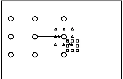
Figure 2.12: The Three Step Search, circles, triangles and squares represent the first, second and third step
13
Figure 2.13: The Diamond Search, circles, triangles, squares, hexagons and stars represent the first,
second, third, fourth and last step respectively 14
Figure 3.1: Filter bank for Multi-resolution Analysis 18
Figure 3.2: (a) Wavelet Decomposition (b) DWT Multi-resolution Analysis of Sample Image Lena
19
Figure 3.3: (a) Redundant Wavelet Decomposition (b) RDWT Multi-resolution Analysis of Sample Image
Lena 20
Figure 3.4: Inter-scale co-efficients regularity estimation for prediction 21
Figure 3.5: The Plot of the red lines in Figure 3.4 in ascending order, shown here in descending order.
21
Figure 3.6: The delineation of the frequencies based on the inter-scale regularity 22
Figure 3.7: S1 cluster of Image Lena (or Lenna) 23
Figure 4.1: First step of the proposed image super resolution algorithm 26
Figure 4.2: Multi-resolution analysis using RDWT, the co-efficients across scales is analyzed. 27
Figure 4.3: Frequency delineation based on areas of strong regularity 28
Figure 4.4: The steps for prediction and refinement of the unavailable detail co-efficients 31
Figure 4.5: Temporal filtering of the wavelet sub bands, derived from the input frames 32
Figure 4.6: Generation of the changes across two input frames 33
pg. x
Figure 4.8: The implementation of the three step process for video super resolution 35
Figure 4.9: The final step of the optimal implementation of video super resolution 36
Figure 5.1: The generated High Resolution image based on the zero-valued detail co-efficients 38
Figure 5.2: The prediction of co-efficients for wavelet based super resolution 39
Figure 5.3: The predicted interpolated frame and the actual frame (frame 6), the PSNR qualities of frames
42
Figure 5:4: Interpolated frames from the temporally related sequence, showing noise and occlusion effect
pg. xi
LIST OF ABBREVIATIONS
SR: Super Resolution
HR: Higher Resolution
LR: Lower Resolution
PSNR: Peak Signal to Noise Ratio
RDWT: Redundant Discrete Wavelet Transform
DWT: Discrete Wavelet Transform
MRA: Multi-Resolution Analysis
Pixel: picture elements
MSE: Mean Square Error
MAD: Mean Absolute Deviation
pg. 1
CHAPTER 1: Introduction and Research Objective
1.0
Introduction
The capture and conversion of continuous time signal to digital samples (or discrete-time signals), is a
core requirement for the current body of processing techniques available for digital electronics. The
proximity and resemblance of the discrete-time signal to its analog counterpart, is measured by the
sampling resolution. This determines the level of (and/or possibility for perfect) reconstruction of the
original signal. However in the design of digital signal processing systems, the application requirement
largely determines this feature as several constraints, limitations and design specifications constitute the
central objective of such systems. This scenario is evident in the general classification of digital image
and video processing devices according to the capture and rendering capabilities.
Meanwhile the deep penetration of this technology and the sheer ubiquity of its availability have created
scenarios of interchangeable and multi-functional usage where for example images captured on humble
mobile phones can end up being primary source material for gait recognition, this results in digital signal
processing problems that require the upward conversion of the resolution of digitally sampled signal.
Moreover, digital video capture, distribution and utilization has become increasingly commonplace due to
significant advances in camera technology, digital circuit integration and storage systems among a host of
other factors. The pervasive deployment of the technology on diverse platforms with wide application
requirements and varied use case scenarios has created a multi-platform creation and consumption chain
where digital video from a broad spectrum of capture devices can be utilized on an equally wide variety
of rendering devices.
The digital image processing devices generate images with specific spatial properties, lower resolution
images are coarsely sampled version of the higher resolution ones, and are intended for devices with
compatible display resolution.
However, usage scenarios and application requirement in the ubiquitous multimedia applications
environment ultimately results in the need for increasing the spatial dimensions of an image. This need is
further compounded by the fact that the lower resolution version of the image could be the only available
media source, this inevitably results in an overarching constrain that requires the extraction of unavailable
details, as the level of information available in images are statistically defined by their resolutions because
pg. 2
This presents a scenario where the only course of action for increasing the resolution of an image is the
direct replication of the available information to the desired levels of spatial dimensions. This approach
results in images with jagged edges and sharp discontinuities. The resulting images show visually
disturbing artifacts and perceptually unnatural image edges lines that considerably distort the images.
However the generated higher resolution output can be enhanced to remove these distortions by
synchronizing the sharp edge gradients into a continuous and smooth curves exhibiting natural rhythm.
The artifacts can also be eliminated by performing a similar action on the non edge portions of the image.
This generally results in perceptually acceptable version of the image but confronts the problem of
blurring. The post pixel replication actions intended for the removal of distortions also eliminates the
variations of the pixels across the images, hence the generated higher spatial resolution image is blurred
in comparison to the original lower resolution input. Several methods for increasing the resolutions of an
image offer solutions aimed at managing the twin problems of sharp discontinuities and blurring, with an
objective / expectation of finding the right balance between these two competing interests. Within the
context of this problem definition, the blurriness of the spatially higher resolution output is a permanent
feature of methods that adopt this model, hence are subject to some severe limitation on performance due
to this conflict.
Alternative formulations of the problem of increasing the resolution of an image has sought to escape this
balancing act by attempting an actual recovery of the lost information in an image due to coarse (under)
sampling in the lower resolution input. These methods leverage on the similarity of the samples on the
digital image to predict the missing samples, such methods adopt complex algorithms and employ
possible background information to generate higher resolution versions of an image from lower resolution
input. However, the prediction of unavailable information carries the twin outcomes of success or failure,
where the failure could result in serious distortions of the image to the level of diminished utility. In
addition, most of the prediction methods provides no feedback mechanism and /or prediction
measurement metric to ascertain the level of deviations of these predictions from the norm. This is partly
because the unavailability of the actual data set prevents the implementation of such mechanisms; this
invariably consigns the usefulness of these algorithms to the accuracy of their models and ultimately
providing no guarantees of success.
More so the video temporal resolution follows the similar principle as the spatial resolution, the digital
video frames are sampled at specific rate, referred to as frame rate, this process is also irreversible and
information lost due to low sampling rates cannot be recovered. The generation of higher temporal
resolution from video sequences with low temporal resolutions can be achieved by estimating the
pg. 3
be estimated, interpolated and applied to generate the intermediate frames lost due to under-sampling.
However methods for estimation of displacements and other inter-frame relationships involves
computationally prohibitive calculations for accurate determination, this stems from the fact that the
displacements and changes from real world scenes are difficult to model in terms of low level blocks of
pixels. This leads to the adoption of high level techniques that certainly and successfully retrieve
advanced displacements and complex inter-frame relations at a very high computational cost that
completely erodes the usefulness of such techniques in real-time applications.
The challenge of providing an optimal combination of estimation accuracy and processing cost is very
central to the task of increasing the temporal resolution of the video sequences.
Up-conversion techniques termed super resolution has been the subject of several research efforts in
signal/image processing and presents enormous challenge because of the unavailability of the original
signal hence focus on the up-sampling of the already digitally sampled signal.
Video super resolution is broken into two sets of techniques for spatial and temporal super resolution. The
spatial super resolution as the name implies provides techniques for increasing the resolution of
images/individual video frames. This consists of two dimensional digital signal processing techniques for
up-sampling, re-sampling, enhancing and/or increasing the resolution of two dimensional digital samples.
The temporal super resolution provides a set of techniques for increasing the frame rate and the associated
inter-frame temporal relationships.
The research presented in this thesis is structured according to two blocks of functional techniques for
video spatial and temporal super resolution. The final optimal combination of the two sets of techniques is
provided in the application example of video super resolution.
1.1
Objective and Purpose of Research
The objective of this research effort is the development of state of the art video super resolution, that
improves on the performance of existing techniques, this goal is accomplished in the following two steps:
1. Research and development of video spatial super resolution that attempts to actually increase the
resolution an under-sampled image or provide methods for improving the performance of current
pg. 4
2. The research and development of temporal super resolution, that relies solely on two input frames to
create interpolated frames between the frames in accurate inter-frame relations and objective precision to
enhance the resolution.
1.2
Layout of thesis
The thesis is presented in the following structural layout, chapter one is this introduction, chapter two
provides background information review, the third chapter provides detailed information of the work
done; chapter four is the implementation of the research proposal. Chapter five is the test and comparison
of the proposed techniques with pre-defined objective criteria, it provides performance analysis and
chapter six is conclusion with additional insights on future work; and the references are provided after the
last chapter.
1.3
Summary
The problem of increasing the spatial dimension (or resolution) of images has evolved from the
exploration of techniques for enhancement of the image for visually / perceptually acceptable quality
levels through the elimination of spikes, discontinuities and uncharacteristic variation in the statistical
distribution of image pixel coloration to the attempting of an actual recreation of the original content. The
temporal super resolution methods, is essentially the determination of the contiguous / coherent changes
across frames and the replication of the changes in an intermediate frame in half measure.
pg. 5
Chapter 2: Background Information Review
2.0
Introduction
Super resolution refers to the techniques used for increasing or enhancing the resolution of an image or
video. The task of increasing the number of individual elements in a sparse data set has a long history,
with deep origins in the interpolation theory. Interpolation as defined by Thiele [1, 2] in 1909 is referred
to as the art of reading between the lines in a table. This functional definition has survived the various
extensions, modifications, transformations and applications of the concept. Reading between the lines
with an aim of increasing the sample size of the data set is a core application tool in signal, image and
digital video processing. The overview of methods for super resolution is presented for spatial (image)
and temporal resolutions respectively.
2.1
Spatial (or Image) Super Resolution
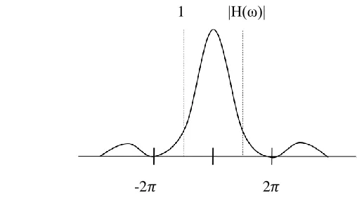
The earliest methods for increasing the vector dimension (or spatial resolution) of an image is the basic
interpolation function known as the nearest neighbor [3], in this method the value of the new (or
interpolated) point is a direct replication of the previous point. This method is equivalent to convolving an
image with a rectangle function (Figure 2.1), which can be interpreted as multiplication with a sinc
function in the frequency domain (Figure 2.2).
1 h(t) 1 |H(ω)|
t w
-1 1 -2 2
Figure 2.1: Nearest Neighbour time domain Figure 2.2: Frequency domain, Nearest Neighbour
The resulting image from this method has sharp discontinuities and is shifted with regard to the original
pg. 6
addition, the frequency attributes of the output image and the original are exactly the same with a simple
linear phase shift.
The linear interpolation (bi-linear for 2D), is an improvement of the nearest neighbour algorithm in which
the new (interpolated) point is derived from the interpolation of two adjacent neighbours. The linear
interpolation can be implemented as the convolution of the image with the triangle function. The process
results in a low pass filtering in the frequency domain (Figure 2.3 and Figure 2.4) with strong smoothing
in the cut-off frequency.
h(t) 1 |H(ω)|
t w
-1 1 -2 2
Figure 2.3: Linear Interpolation time domain Figure 2.4: Frequency domain Linear Interpolation
The cubic (bi-cubic for 2D) interpolation [4, 5, 6] also improves on the linear interpolation by using three
points instead of two, as a result of this extension, the interpolated image is smoother. The cubic
interpolation is implemented using cubic convolution in the spatial domain. This results (see Figure 2.5
and Figure 2.6) in a low pass filter with smoother cut-off frequency response in the frequency domain.
t w
-1 1 -2 2
pg. 7
The cubic interpolation can also be implemented using the Lagrange polynomials and cubic B-splines.
However, additional methods of image super resolution exists, these include the many variations of
splines. The concept of piecewise polynomials with smoothly separated units‟ points has been in
existence in various shapes and forms and was formalized by Schoenberg [7] in 1946 as splines.
Splines can be described in terms B-splines expansion where B stands for basic:
s(x) = (2.1)
Equation 2.1 represents the integer shifts of the B-spline of degree n, the c(k) are the B-spline
co-efficients. B-splines are constructed from rectangular function ß defined as ßn(x).
ß0 = (2.2)
(2.3)
(n+1 times)
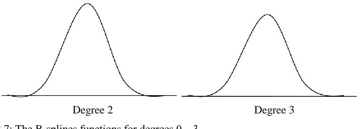
B-Splines of degree 0, 1 and 2 are piecewise constant, linear and cubic respectively (see Figure 2.7);
higher degrees can be easily constructed from the basic splines known as B-splines.
pg. 8
Degree 2 Degree 3
Figure 2.7: The B-splines functions for degrees 0…3
The cubic B-spline is very popular in image processing due to its curvature and can be derived from the
B-spline as presented below in Equation 2.4:
(2.4)
However, direct low pass filters has been designed for increasing spatial resolution, several methods with
varying low pass response(s) (see Figure 2.8) exists, these are designed to achieve a smooth pixel
inter-relationships across interpolated points. The two dimensional (2D) recursive (IIR) filters [8] is a typical
example, however other versions with FIR implementations also provides comparative performance at
additional high computational cost. In addition separable two dimensional filtering is also used for lower
computational cost with the obvious downside of performance penalties.
Figure 2.8: Typical design response(s) for low pass filters used for resolution enhancement.
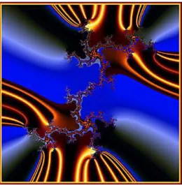
Fractal zooming is another method of increasing the resolution of an image, it is derived from fractal
pg. 9
or compressed using geometric transformation functions. In fractal compression, the compressed image is
resolution independent, this stems from the premise that images are characterized as fractals which is
defined as a loosely connected conflagration of self-similar objects. This definition contends that fractals
possesses no physical characteristic sizes, rather strictly self-similar units with metric properties defined
on the atomic level, hence the overall arrangement is scale independent. Self similarity in fractal parlance
is defined by the expression below in Equation 2.5:
(2.5)
M(x) represents any metric property of the fractal (e.g. area or length), and x denotes the scale of measurement of the metric property, r is a scaling factor, such that 0≤ r ≤1 and f(D) is a function of the fractal dimension D for the given metric property.
An example of the fractal coding method as originally introduced by Von Koch known as Von Koch
Curve or Snowflakes is presented in Figure 2.9.
1.
2. 4.
3.
Figure 2.9: Van Koch Curve or Snow flakes, the rule is repeated at every stage
The Von Koch curve example in Figure 2.9 shows the different transformation of the original line, this
simple illustration is at the heart of fractal coding theory, in which every image is decomposed into
pg. 10
rules on these units to recover the original image. However since the atomic units is the sole content of
the entire image, the decoding process can recover the image to any desired scale independent of the
original. However, despite the promising nature of the theory and the utter usefulness of its application,
Fractal coding is yet to gain traction due to the prohibitive computational cost of the encoding process.
Several attempts at simplifying the process with wavelet-based decomposition have been proposed [12]
and remain a strong focus of research efforts. Examples of fractal generated images are presented Figure
2.10.
Figure 2.10a: Example of fractal generated Image
pg. 11
The wavelet based methods are the latest additions to the litany of super resolution algorithms. The
unique contribution of this group, of super resolution techniques is the focus on the possibility of
increasing the resolution (the spectral content) of a signal rather than enhancement. Common and central
to all wavelet based techniques is the multi-resolution analysis of the input signal into several resolutions
or scales and reliance on the structural self similarity evident across the scales to predict the next higher or
finer scale of detail co-efficients (see Figure 2.11). However the divergence in approach occurs on the
method of prediction, the Hidden Markov tree [13], have been used to predict the next set of co-efficients
using training data from a large pool of images. The wavelet co-efficients at the finest scales is predicted
based on the state transition probabilities across the scales and the determination of an expected value of
the state of the co-efficient at the finest scale. The method also features a sign prediction algorithm where
the predicted magnitude of the finest scale co-efficients is assigned a positive or negative sign based on
the sign transitions of its ancestry.
pg. 12
More so additional modification [14] has been made to this method where the requirement for training is
eliminated and the co-efficient sign prediction method simplified, resulting in improved comparative
performance. However, the two methods follow a tightly coupled quad-tree inter-scale dependency
where the magnitude of the parents propagates to child co-efficients, however the quad-tree structure
provides a potential pitfall for this approach for higher levels of iterations as low magnitude parents often
yield very high magnitude in the child co-efficients due to shifts. More so the simplified co-efficient sign
prediction directly extends the sign of the parent to the children, this approach though computationally
efficient is fraught with potential errors. Directional wavelet filtering [15] has been used to improve the
performance of increasing resolution, it attempts to create multiple and flexible directional filtering
radically different from the traditional horizontal and vertical separable two dimensional filters in order to
closely model the characteristics of the image edges, the performance of the method lags standard wavelet
methods in complex images though it provides marginal gains in less complex ones. Neural network
method has been proposed [16], and an edge adaptive method using Markov chain Monte Carlo is also
proposed [17], in addition several statistical and algebraic methods exists, but these methods lacks a
definitive model that constrains the feasible solutions space for the predicted co-efficients, hence rely
heavily on the validity and accuracy of the model to achieve desired results.
2.2
Temporal Super Resolution
Methods for increasing or enhancing the temporal resolution of video sequences include the simplistic
replication of frames, in which the video frames are simply repeated in order to increase the frame rate.
Beyond this method, other approaches are deeply rooted in, and practically synonymous with the motion
estimation techniques for eliminating redundancy across video frames. However the application of this
technique to super resolution requires the interpolation of the motion vectors for motion compensated
prediction of the interpolated frame; this is commonly referred to as motion compensated interpolation for
video format conversion (MC-VFC).
Frames with temporal proximity in video sequences generally contain little variations in content; a greater
percentage of the variations can be grouped as motion of objects (group of pixels) in the frames. Motion
estimation of pixels of a video frame is the focus of several research efforts, past and ongoing, several
techniques has been proposed, implemented, deployed and/or modified. Majority of the existing
algorithms provide a model of the motion estimation problem as the determination displacement vectors
of a fixed and variable block of pixels in a frame, while this is uncharacteristic of motion in video
pg. 13
based motion estimation methods that leverages on object segmentation provides greater precision and
accuracy in this regard, but this approach is computational prohibitive, within the context of the state of
current implementations, for any practical usage in digital video processing applications requiring low
processing latency. Prominent block based motion estimation algorithm includes the Full Search (also
known as Exhaustive Search or Global Search), this method provides the best results among all matching
algorithms due to its exhaustive search of the target frame for the best match for the candidate block of an
image sequence. However, the approach is very computationally expensive and is rarely used. Other
methods like the three step search, attempts to achieve the quality performance of the full search with far
lower computational cost, this method employs a three step hierarchical search method (see Figure 2.12)
where the search area is constantly refined according to a cost function and the new search area is defined
that represents the best target for matching the candidate block. Additional modifications to this method
include the New Three Step Search [18], Simple/Efficient Search [19] and the Four Step Search [20].
Figure 2.12: The Three Step Search, circles, triangles and squares represent the first, second and third step
respectively
Several hybrid and modifications of these search patterns have been proposed and implemented, these
include the Diamond Search [21], and this is an extension of the four step search but differentiates from it
by adopting a diamond search point pattern instead of a square. The search method uses two fixed size
diamond shapes, called the large diamond search pattern and the small diamond search pattern (see Figure
pg. 14
best match, the hierarchical refinement is implemented with large diamonds until the last step, when the
small diamond is actually used.
Figure 2.13: The Diamond Search, circles, triangles, squares, hexagons and stars represent the first,
second, third, fourth and last step respectively
There are related methods derived from the methods presented, these derivations include extensions like
the adoption of the complex shaped polygon patterns and variable shaped patterns. The diamond search
method provides comparable quality performance to the Full Search and provides the basic structure for
most existing extensions in literature.
However the quest for efficient and accurate motion estimation across video sequences is not limited to
spatial domain techniques, the fix all wavelet phenomena has not spared this area of digital video
processing, there are currently two evolutions in this area, the first is the multi-resolution motion
estimation (MRME) methods that tend to create efficient method for motion vector determination at
different levels of resolution without repetitive processing. The second line of approach is the
wavelet-based motion estimation that focuses on traditional motion estimation but with a new wavelet wavelet-based
technique. Multi-resolution motion estimation (MRME) typically involves the estimation/determination
of motion vectors at either coarsest or finest scale, followed by subsequent refinements of the vectors
across the hierarchical structure in either directions, implementations of MRME include a premier work
and widely referenced material [22], other research work in this field includes [23], more so an analysis
pg. 15
the finest to coarsest vector estimation and refinement approach provides superior performance. This
result completely undercuts the super resolution potential of the coarsest to finest approach, as it would
have provided a perfect fit to the problem formulation of wavelet based video super resolution.
Wavelet based motion estimation adopts multi-scale (resolution) sub-band based matching, in this
scenario, the target area/blocks in each wavelet reference sub-band is matched to the corresponding
current sub-band, additional approaches includes the use of redundant wavelet transform for sub-band
matching. More so the wavelet based motion estimation techniques has recorded a giant leap in
comparison to the established spatial domain methods, the best results presented [25] in this area as at the
time of writing this thesis is competitive to the spatial domain approach in terms of quality though lags it
severely in resource requirement.
2.3
Summary
The video spatial (image) super resolution methods with the exception of wavelet and fractal methods,
provides an enhancement of the lower resolution image, this approach though practical and pragmatic in
the face of the sheer impossibility of recovering the under-sampled information, provides a very strong
limitation, such that the higher resolution (HR) image, is essentially as good (if not worse) as the lower
resolution version, thereby paving the way for the exploration of techniques for the recovery of lost
spectral content. The motion estimation methods for temporal super resolution, provides search methods
for handling translational motion of blocks of pixels. Several existing propositions and algorithms,
pg. 16
Chapter 3: Proposed Video Super Resolution
3.0
Introduction
Video super resolution is accomplished in two steps, spatial and temporal; each of these steps requires
distinct set of techniques for its implementation. The proposed methods are presented in that order, in the
following three sections, the first section provides details of the proposed spatial (or image, it is used
interchangeably throughout this text) super resolution, the second section deals with the temporal
techniques and the third and final section provides an optimal combination of the two bodies of
techniques to implement video super resolution.
3.1
Video Spatial (Image) Super Resolution
The main purpose of this work is to generate an output that is greater in spatial resolution than the original
input and conforms to the statistical/spectral dynamics of the image at this new spatial resolution.
However achieving the latter remains a daunting task owing to the fact that the Super Resolution (SR)
algorithms are technically constrained to up-sampling of already digitally sampled signal. Several SR
methods as described in chapter two provides an enhancement of the resolution at higher spatial
dimensions owing to this challenging constraint. However wavelet based groups of techniques provide
the possibility of increasing rather than enhancing the resolution of an image. This approach provides a
platform that supports the probable recovery of lost image details due to under-sampling. The proposed
video spatial SR method leverages on this possibility to attempt a recovery of high resolution image from
the lower resolution version, using it as the only input.
The problem model and the detailed description of wavelet theory strictly within the context of spatial
(image) super resolution is presented in the following sections succeeded by the proposed technique based
on the model.
The problem definition: The proposed super resolution model is defined for a single constrain, it applies
to band limited signals. For a continuous time one–dimensional signal f (t)
(2)
there exist a certain frequency q for which |w| > q, F(jw) = 0; where (2) is the Fourier transform of the
pg. 17
(3.0a)
, m = 0
(3.0b)
This signal can be reconstructed perfectly from the discrete time version. Hence the super resolution
problem can be characterized as the increase of the sampling frequency from a level (< 2q) to any desired
level, with a maximum limit at the Nyquist limit (> 2q). To achieve this objective, a frequency domain
solution that attempts to recover the higher frequencies beyond the range the signal are sampled is
proposed. In this approach, the spectral distribution of the input signal is used to predict the
lost/unavailable frequencies. To explore the frequency properties of the signal, wavelet multi-resolution
analysis is applied; this provides the advantage of time-frequency [26] characterization of the signal
unavailable in Fourier transform.
For wavelet transform of an input signal x (t) the output wavelet co-efficients Cs,τ .
is the wavelet function, s is scale (1/frequency), and is time shift. The inverse is the linear
combination of the wavelet at all scales and translations.
However, the signal can be approximated to a desired resolution (scale) s=A, in which case the
approximated version of the original signal is xA(t).
The difference between the approximated version at s=A and the original signal
pg. 18
For discrete time signals the approximation is represented by equation (9) where h (nT) is the impulse
response of the wavelet function.
The difference is the convolution of the input signal with a high pass filter g(nT) which is related to the
approximation (low pass) filter as shown in equation 10
g (L – 1 – nT) = (-1)n h(nT) (10)
where L is the filter length
Multiple approximations of the original signal at different scales (resolutions) with the resulting
differences at each level constitute the much-famed wavelet multi-resolution analysis (MRA). This is
typically implemented in a filter bank as shown in Figure 3.1, derived from sub-band coding.
Input
Figure 3.1: Filter bank for Multi-resolution Analysis
Multi-resolution analysis can be defined [27] as a sequence of spaces {V j} jЄz of L²(R) with respect to a
function if the following constraints are true.
(j, k) Z², f (t) Vj ↔ f (t – 2 j
k) Vj (11.1)
j Z, Vj+1 Vj (11.2)
j Z, f (t) Vj ↔ f ( ) Vj+1 (11.3)
H
G
H
G
H
G
H
pg. 19
Vj is translation invariant proportional to scale 2 j
, equation (11.1), while equation (11.2) states the
causality property, equation (11.3) specifies an approximation of the original signal at coarser resolution,
more over all details of the signal is lost when the resolution goes to zero as shown in equation (11.4), and
inversely (11.5) the original is recovered as resolution tends to infinity. In the wavelet based SR process,
the LR input constitutes the approximation, while the difference is predicted. Wavelet multi-resolution
analysis provides a tool for estimation of the relative similarity of the differences across scales, useful in
predicting the next higher set of unavailable differences for which the input signal is the approximation.
The wavelet decomposition of signals into approximation and difference components, results in output
wavelets co-efficients with same sample size as the original signal for each component. For two
dimensional signals like images, the wavelet transform co-efficients will be four times the original image
size, however for perfect reconstruction of the original input, only half of the wavelet co-efficients (in
both directions) is required as this can be accomplished using either the set of even or odd co-efficients,
this leads to the subsampling of the wavelet co-efficients used in discrete wavelet transform (DWT), as
the original output is considered redundant or over-complete for reconstruction. However the output
sub-sampled version (DWT), is altogether complete for perfect reconstruction but individually incomplete, as
each component suffers from shift variance, due to subsampling, more over within the context of
multi-resolution analysis, iterative subsampling greatly reduces the usefulness of co-efficients for inter-scale
frequency analysis as the increasing reduction of samples sizes results in increasingly low frequency
resolutions completely unsuitable for such analysis. This leads to the adoption of redundant discrete
wavelet transform for inter-scale frequency analysis.
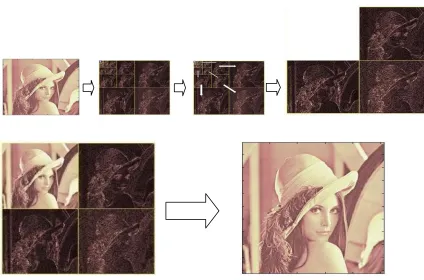
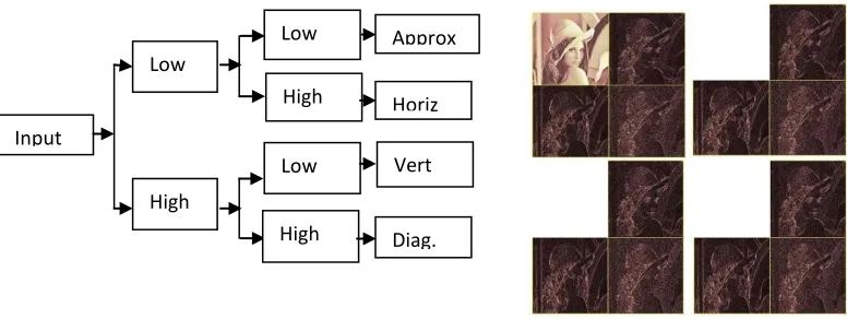
Figure 3.2: (a) Wavelet Decomposition (b) DWT Multi-resolution Analysis of Sample Image Lena
pg. 20
Figure 3.3: (a) Redundant Wavelet Decomposition (b) RDWT Multi-resolution Analysis of Sample Image
Lena
The inter-scale analysis of the high frequency components (Horiz., Vert., and Diag.) of the resulting
wavelet co-efficients accomplishes two goals: (1) The determination of the existence of sufficient high
frequency information in the image, which is pre-requisite for the proposed image super resolution
algorithm (2) It provides a useful resource for the detection of the resolution invariant features of the
image, detection of these features provides the unique frequency characterization of the image. The
details of the two design objectives are presented below:
Spectral content pre-requisite: The proposed algorithm relies on the higher ranges of frequency content,
therefore the prior establishment of the availability of this crucial information is necessary to guarantee
any performance. This is established by the estimating the regularity of the wavelet co-efficients across
the scales in fine to coarse order as shown in Figure 3.4, 3.5, 3.6.
Input
High Low
High Low
High Low
Approx
Horiz
pg. 21
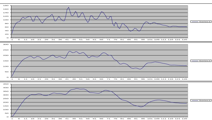
Figure 3.4: Inter-scale co-efficients regularity estimation for prediction
Figure 3.5: The Plot of the red lines in Figure 3.4 in ascending order, shown here in descending order.
0 20 40 60 80 100 120 140 160 180
1 6 11 16 21 26 31 36 41 46 51 56 61 66 71 76 81 86 91 96 101106111116121126
Series 1
0 50 100 150 200 250 300
1 6 11 16 21 26 31 36 41 46 51 56 61 66 71 76 81 86 91 96 101106111116121126
Series 1
0 50 100 150 200 250 300 350 400 450
1 6 11 16 21 26 31 36 41 46 51 56 61 66 71 76 81 86 91 96 101106111116121126
pg. 22
Figure 3.6: The delineation of the frequencies based on the inter-scale regularity
In the Figure 3.6, the S3 cluster shows a distinct regularity with increasing magnitudes from finest scale
to the coarser scales. The S3 cluster must exist in an image for any guarantee of performance, as the
method relies on the enforcement of the equality constraint on the image features grossly dependent on
the spectrum range. Images (see Figure 3.7) adjudged by this process as having insufficient higher range
spectrum content typically lack feature detail that can be reliably enforced on the estimated higher
resolution version.
Resolution Invariant Feature Detection: The inter-scale analysis also provides a tool for detection and
estimation of resolution invariant features of the image. The correlation between the co-efficients across
scales within the S3 cluster (Figure 3.6) provides the synchronization points for automatic extraction of
the exhaustive and salient features of the image that transcends resolutions.
However, this is a mathematically involved and computationally expensive process, an alternative
proposition is the use of standard features of an image that are resolution invariant, these include the edge
strength, edge direction and edge continuity. This is adopted in this research.
Succeeding the analysis is the prediction of the unavailable wavelet co-efficients using the Lipschitz
regularity; this provides an estimation of the growth rate across scales. The predicted values are
constrained to conform to the standard features of the lower resolution image, in comparison to the
pg. 23
constraints is a bounded non-linear optimization, where the solution space is confined to the magnitude of
the coarser co-efficients.
Figure 3.7: S1 cluster of Image Lena (or Lenna)
3.2
Temporal Super Resolution
The performance of motion estimation algorithms largely depends on the search and matching methods,
the objective matching criteria has very limited tunable parameters and hence a move from Mean Square
Error (MSE) to the Mean Absolute Deviation (MAD) has been the significant progression in this area.
The central core of the performance for motion estimation algorithms reside in the search methods and all
existing algorithms are defined and differentiated by their search methods. Several algorithms for motion
estimation from the exhaustive search (or Full Search) to the Four Step Search employ diverse approaches
to implementing an optimal search algorithms, which ultimately aim at improving the computational
performance of these techniques, in furtherance to this objective, a new method is proposed that uses
redundant discrete wavelet transform and temporal filtering to extract the changes across video frames
and constrain the search area to the defined regions of the frames temporally associated. The proposed
technique has no close implementation in literature or equivalence for fair comparison, but provides an
pg. 24
The temporal aspect of the video super resolution is modeled as the increase of the frame rate by
generating and inserting intermediate frames between two adjacent frames. This model requires two input
frames temporally related in chronological order and returns an output with a number of intermediate
frames.
The insertion or generation of an intermediate frame is solely based on the accurate depiction of the
temporal relationship across the adjacent input frames. This process derives from techniques and
algorithms that estimate the relative redundancies, differences and displacement across frames. These
methods largely referred to as motion estimation algorithms (as presented in chapter two), employ mainly
objective matching of the areas of the input frames. The proposed algorithm improves on these methods
by restraining/confining the matching target to areas of the input with differences or displacement. This
provides an improved performance and applicability to real-time video processing. The estimated
displacement vectors across the two input frames are interpolated to produce the predicted intermediate
frame(s).
To estimate the difference(s) or displacement across two input frames, redundant two dimensional (2D)
discrete wavelet transform is applied to the frames of the input video, the resulting co-efficients of the
adjacent frames (the approximation and three detail orientations or sub-bands) of the input video are
filtered using high pass reversible integer Haar wavelet filter. The resulting frames from the temporal
filtering contains low and/or near zero magnitude values for co-ordinates with little or no changes across
frames and high values for areas of relative motion. The result of the temporal filtering hereafter referred
to as motion profile is segmented using an adaptive threshold that classifies the values into motion and
non – motion pixels.
In the threshold-based classification process the sorted co-efficients values of the motion profile is
analyzed for sharp rise/relative discontinuity in magnitude, the resulting value from this analysis become
the magnitude threshold. This process can also be accomplished using a simple hard coded threshold
resulting in very minimal outliers. The consequence of obtaining sub-optimal threshold classification due
to the hard coded baseline is the minimal or fringe noise spikes in the motion profile, this is far too low
penalty in comparison the compulsory increase in processing footprint added by the adaptive threshold
method.
The classification scheme is used for predicting the areas of the adjacent video frames with significant
pg. 25
accuracy of this prediction. The co-efficients below the threshold is made equal to zero. A two step 2D
inverse discrete wavelet transform is applied to the magnitude classified wavelet co-efficients detailed
below:
1. The co-efficients are used in two dimensional inverse discrete wavelet transform.
2. The approximation co-efficients are completely replaced with zero and an inverse 2D discrete
wavelet transform is applied.
The image pixels resulting from the two steps process above is added to produce the motion areas of two
adjacent video frames. The generated image is used for block matching where only block within the
motion areas are selected for matching thereby optimizing the performance.
3.3
Summary
The presented video spatial (image) super resolution method, attempts the recovery of the lost image
information due to under-sampling by re-creating it following an established rule (feature constraints),
The extent of the recovery is dependent on the availability of these rules, the detection/creation of the
feature constraints is not considered, additionally the detection of non-standard feature constraints would
extensively enhance the potential robustness and precision of the proposed algorithm. The video temporal
pg. 26
Chapter Four: Implementation
4.0
Introduction
The video super resolution algorithm was implemented in a two step design process of image and
temporal super resolution. The individual merits and trade-off of the methods are analyzed independently,
there after an optimal combination of the two methods for real-time video super resolution is presented.
The presentation in this chapter follows that order.
4.1
Image Super Resolution
The implementation is a five step process listed below:
(1.) Redundant Discrete Wavelet Transform
(2.) Estimation of the growth rate
(3.) Grouping/ Delineation of the Image Frequencies
(4.) Prediction of the coefficients
(5.) Refinement of the predicted coefficients
The details of the steps are presented in the following sections:
4.1.1 – Redundant Discrete Wavelet Transform
Two dimensional separable discrete wavelet transform is applied on the input low resolution (LR) image,
using the Cohen Daubechies Feauveau 9/7 bi-orthogonal filter as shown in Figure 4.1, the filter kernel is
presented in Table 4.1.
pg. 27
Table 4.1: The cdf-9/7 filters kernel used in this implementation is the FBI version
The output of the transform is four times the size of the input. The RDWT is used for Multi-resolution
analysis applied to the next step.
4.1.2 – Estimation of regularity and growth rate
The multi-resolution analysis of the input image is used for estimating the regularity and growth rate of
the wavelet coefficients across scales as shown in Figure 4.2 below.
Magnitude
Scale
Figure 4.2: Multi-resolution analysis using RDWT, the co-efficients across scales is analyzed. Analysis low-pass filter: 0.0267487574108098,-0.0168641184428750,-0.0782232665289879,
0.2668641184428723, 0.6029490182363579, 0.2668641184428723, -0.0782232665289879, -0.0168641184428750, 0.0267487574108098;
Analysis high-pass filter:
0.0456358815571247, -0.0287717631142498, -0.2956358815571235, 0.5575435262284970, -0.2956358815571235, -0.0287717631142498, 0.0456358815571247;
Synthesis low-pass filter:
0.0534975148216208, -0.0912717631142514, -0.1564465330579798, 0.5912717631142532, 1.2058980364727310, 0.5912717631142532, -0.1564465330579798, -0.0912717631142514, 0.0534975148216208;
Synthesis high-pass filter:
0.0337282368857512, -0.0575435262285022,-0.53372823688575,
1.1150870524570070, -0.5337282368857500, -0.0575435262285022, 0.0337282368857512;
pg. 28
4.1.3 – Wavelet coefficients grouping and delineation
The frequency distribution of the image from the multi-resolution analysis is used for the estimation and
delineation of the wavelet bands into groups based on regularity. The existence of S3 cluster in the image
is a core requirement for the proposed method, the delineation is shown in Figure 4.3. The inter-scale
relationship across the finer scales is estimated using the Lipschitz regularity [27], this defines the
calculation of the growth factor termed Lipschitz exponent. To calculate the Lipschitz exponent, the
absolute maximum value for the coefficients on the finest (first set of coefficients from the MRA) scale is
found, and the slope of the log2 of both the coefficient and that of the absolute value of the coefficient in
the same position in the next higher scale is the Lipschitz exponent for these two adjacent scales.
pg. 29
4.1.4 – Prediction of coefficients
The next higher set of coefficients of the wavelet sub-bands is predicted using the regularity relations of
the coefficients across scales within the S3 cluster, the steps of the prediction is presented in Figure 4.4
below.
(1.)The original LR input image:
pg. 30
(3.)The detail coefficients are predicted using the regularity of the coefficients from S3 cluster.
pg. 31
(5.) The predicted coefficients are refined using the comparison of the standard, resolution invariant
features in the generated HR images and the original LR input.
Figure 4.4: The steps for prediction and refinement of the unavailable detail coefficients.
The edge strength is used in the implementation; the refinement process is restricted to selection of the
best comparative result for the standard feature within the range of the magnitude of the (preceding)
coarser coefficients in the same position.
4.2
Temporal Super Resolution
The implementation of the Video Temporal Super resolution is also a five step process as presented
below:
(1.) Redundant Discrete Wavelet Transform of input frames
(2.) Inter-frame (temporal) filtering of RDWT´ed frames
(3.) Application of a value threshold on the results of (2.)
(4.) Inverse RDWT of the results of (3.) and the Inverse RDWT of the results of (3.) with the
approximation coefficients made equal to zero. The two results of (4.) is added together to produce the
motion profile of the adjacent frames.
pg. 32
(5.) The motion profile is used deterministic search and matching across the input frames for estimation
of the differences and displacement vectors.
The individual steps of the process is presented in the next sections
4.2.1 – Redundant Discrete Wavelet Transform of input frames
This is the single decomposition of the input frames into wavelet sub-bands, similar to the first step in
image super resolution technique. However temporal super resolution receives two input frames.
4.2.2 – Temporal (inter-frame) Filtering of the wavelet sub-bands
The output of the first step for the input frames is temporally filtered using the Haar integer reversible
high pass wavelet filter, as shown in Figure 4.5 below:
pg. 33
4.2.3 – Threshold classification
The application of threshold classification to the temporally filtered coefficients, is used to eliminate the
near zero values. The hard magnitude threshold is applied to the output.
4.2.4 – Inverse DWT and Inverse DWT with zero values in approximation coefficients
Inverse discrete wavelet transform of the output of step 3 above, and the output an inverse discrete
wavelet with the filtered approximation coefficients replaced with zero values is summed up to produce
the motion profile of the two frames, all non zero values in the motion profile are areas of relative motion
across the frames, this is shown in Figure 4.6.
pg. 34
4.2.5 – The motion profile is used for deterministic search and matching across the input frames for
estimation of the displacement vectors.
The estimation of differences and displacement vectors across the input frames is restricted to the areas of
changes across the frames, as defined by the motion profile. The objective criteria and the shape and size
of the matching units (regions or blocks) used are user defined, any method can be implemented. An
example is shown in Figure 4.7 below:
Figure 4.7: An example of estimation of areas of changes across two input frames
4.3
Video Super Resolution
The key modifications for optimal combination of the two techniques are presented in the following sub
sections.
4.3.1 Optimal Combination of the Spatial and Temporal techniques for Video Super Resolution
The optimal combination of the techniques for efficient and possible real-time video super resolution is
implemented by adding the following modifications to the steps in the spatial and temporal super
resolutions. The following modifications are implemented:
1. The image (spatial domain) feature constraints is restricted to standard features (Edge Strength,
Direction and Continuity), therefore eliminating automatic detection process, however only the
edge strength feature constrain is implemented, additional optimizations can be achieved by
streamlining the constrain implementation.
2. The estimation of the regularity (or growth) is eliminated to optimize for speed, requiring only
pg. 35
3. The predicted coefficients are therefore directly derived from the last available scale.
4. The refinement process is implemented using the binary search method.
The resulting optimally combined spatial (image) and temporal super resolution is a three step process as
shown in Figure 4.8 and 4.9:
Step 1. Single decomposition
Step 2. Refinement and Temporal Filtering
Step 3. Apply the Refinement factor and perform Inverse DWT
pg. 36
Figure 4.9: The final step of the optimal implementation of video super resolution
4.4
Summary
The implementation steps of the image super resolution algorithm support resource efficient offline or
online applications, with several tunable parameters. However the detection of resolution invariant
features was not implemented, this can be achieved for offline applications using dual frequency
approach, where correlation of the frequency of the wavelet coefficients across resolutions can be
extracted. The temporal resolution method provided an efficient extraction of motion across frames;
however the choice of wavelet filters (CDF9/7), is solely based on the need to conform to the image super
pg. 37
Chapter Five: Experimental Analysis and Results
5.0
Introduction
The test and analysis of the performance of the proposed video super resolution is presented in two
sections following the order established throughout this thesis, the first sections provides details of the
test environment and benchmarks for image super resolution while the second section provides the
comparative analysis of motion estimation functions of the temporal super resolution against other similar
algorithms. The tests are presented in the following sections:
5.1
Test and Performance Analysis of Image Super Resolution
The establishment of baseline or benchmark for performance analysis of image super resolution
propositions follows a general rule that tends to adopt bi-linear and/or bi-cubic interpolation. However
this is inadequate for wavelet based methods [28], as all wavelet based methods will easily outperform
bi-linear and bi-cubic interpolation, therefore a more accurate model for comparison is the objective
measurement of the peak signal to noise ratio of generated HR image based on predicted coefficients
against the zero valued coefficients.
The zero-valued coefficients provide the maximal proximity of the image at that resolution to the target
HR version; this can be easily proved using any other spectral methods. The resulting HR estimate from
the zero-valued detail coefficients version (shown in Figure 5.1) provides the equivalence of increasing
the spatial domain resolution (more accurately dimensions) without the attendant increase in the spectral
pg. 38
Figure 5.1: The generated High Resolution image based on the zero-valued detail coefficients
This provides the required benchmark for algorithms that attempt to introduce additional spectral
information through prediction and other methods. These propositions or algorithms MUST outperform
the zero-valued detail coefficient HR image in order to lay claim to any useful contribution and/or
additional insight in the quest for improving/enhancing image super resolution. However outperforming
zero-valued HR version is a very difficult and daunting task, this stems from the fact that predicting the
unavailable information lost through under-sampling with any degree of certainty is almost technically
untenable. For example (Figure 5.2) using the LR Lenna image of resolution 256x256 and generating a
higher resolution version (512x512), will require the prediction of 3x256x256 detail coefficients, ALL the
predicted values MUST be within the range of the actual values in order to outperform the zero-based
version of the HR image, or else the prediction of the coefficients will result in a deterioration. The
fluidity of the process makes the odds for accurate prediction very low as small errors, perturbations and